Estimating Fuel Consumption of an Agricultural Robot by Applying Machine Learning Techniques during Seeding Operation

Abstract

The integration of agricultural robots in precision farming plays a pivotal role in tackling the pressing demands of minimizing energy usage, enhancing productivity, and maximizing crop yield to meet the needs of an expanding global population and depleting non-renewable resources. Evaluating the energy expenditure is vital when assessing agricultural machinery systems. Through the reduction of fuel consumption, operational costs can be curtailed while simultaneously minimizing the overall environmental footprint left by these machines. Accurately calculating fuel usage empowers farmers to make well-informed decisions about their farming operations, resulting in more sustainable and productive methods. In this study, the ASABE model was applied to predict the fuel consumption of the studied robot. Results show that the ASABE model can predict the fuel consumption of the robot with an average error equal to 27.5%. Moreover, different machine-learning techniques were applied to develop an effective and novel model for estimating the fuel consumption of an agricultural robot. The proposed GPR model (gaussian process regression) considers four operational features of the studied robot: total operational time, total traveled distance, automatic working distance, and automatic turning distance. The GPR model with four features, considering hyperparameter optimization, showed the best performance (R-squared validation = 0.93, R-squared test = 1.00) among other models. Furthermore, three different ML methods (gradient boosting, random forest, and XGBoost) were considered in this study and compared with the developed GPR model. The results show that the GPR model outperformed the mentioned models. Moreover, the one-way ANOVA test results revealed that the predicted values from the GPR model and observation do not have significantly different means. The results of the sensitivity analysis show that the traveled distance and the total time have a significant correlation with the fuel consumption of the studied robot.

1. Introduction

The world’s population is growing, and nonrenewable resources, like fossil fuels, are limited. This makes it urgent to reduce and control energy use in agriculture and other economic sectors [1,2]. By utilizing novel precision agriculture techniques in unmanned operations, agricultural robots can improve agricultural operations’ efficiency by automating agricultural processes, saving operating time, decreasing the amount of energy needed to complete repetitive farming tasks, and boosting crop yield.

In the economic assessment of agricultural machinery systems, the energy cost has significant importance [3,4]. Fuel and oil costs typically account for up to 45 percent of the machine’s total costs, and reducing fuel consumption can cut operational costs and decrease the environmental impact of the machinery [1,4]. Estimating the amount of fuel consumption, which is one of the primary input expenses, can lead to the adoption of proper strategic and operational decisions in various agricultural tasks [5].

Numerous studies in this field have been carried out. Rahimi-Ajdadi et al. [1] presented a backpropagation Artificial Neural Network (ANN) model with six training algorithms for estimating the fuel consumption of a tractor. They used Nebraska Tractor Test Lab (NTTL) data for developing their model. They considered engine speed, throttle and load conditions, chassis type, total tested weight, drawbar, and PTO power as model parameters. The results show that the ANN model shows a better determination coefficient (R-Squared = 0.986) and prediction accuracy (R-Squared = 0.938) than stepwise regression. Lili Yang et al. [6] developed a model for qualitatively recognizing the behaviors and estimating the fuel consumption of a tractor in sowing operations. The model uses principal component analyses and a random forest algorithm to predict fuel consumption in maize sowing operations. The findings demonstrated that there were increases of 2.06%, 8.99%, and 21.79%, respectively, in the harmonic mean of the precision and recall of the sowing, filling, and turning behaviors. Kichler et al. [7] presented a technique to use two deep tillage implements to examine the impact of transmission gear choice on fuel costs, draft, and other equipment performance characteristics. Transverse and vertical draft forces, as well as tractor fuel consumption, slip, axle torque, and engine rpm, were all monitored in real-time. According to the results, the fuel consumption rate increased by 105%, the implementation draft increased by 28%, and the power increased by 255% between the slow and rapid speeds. Kocher et al. [8] offered five models to calculate fuel consumption for tractors used in agriculture that have partial drawbar loads. The findings demonstrate that there was no statistically significant difference between the fuel consumption model (model 5) and the model as a linear function of drawbar power on concrete, travel speed, and engine rpm. Model 5, which has a single equation that works for the whole speed range examined, was found to be the most accurate of the five models for estimating fuel consumption based on the data. Kim et al. [9] developed a mathematical model to estimate the fuel consumption of tractors using OECD tractor test data by considering the throttle, engine power, load, and PTO speed of the tractor as input parameters of the model. The results show that the percentage errors of the predicted fuel consumption ranged between 0.11 and 4.67%. Grisso et al. [10] created a generalized fuel consumption equation under the assumption that fuel consumption may be estimated from data collected at full throttle and from engine speed reduction percentages. The research included three factors: the rated PTO power, the percentage of reduced engine speed for a partial load from full throttle, and the comparable PTO power to the rated PTO power. Paraforos and Griepentrog (2019) [11] used a CANBUS data logger to gather fuel rate data while using a mounted, reversible moldboard plow. The DGNSS receiver received GPS data, which was then modeled and simulated using Markov chains. These chains demonstrated the ability to represent the operating mode switching that occurs during headland turning. To obtain various realizations of the scenarios they examined, they ran 10,000 Monte Carlo simulations. When compared with the observed total fuel consumption, their suggested methodology was able to estimate the total fuel consumption with a mean difference of 0.9% and a 3.7% standard deviation. Naik and Raheman (2019) [12] developed a model for the fuel consumption of a two-wheel-drive tractor in tillage operations. A tractor equipped with a rotavator was the subject of field tests at seven distinct engine speeds (ranging from 35 to 75 percent of maximum engine speed), gear ratios (L2 and L3), and operating depths (60, 80, and 100 mm). There is a correlation between the tractor’s fuel consumption and its operating depth, engine speed, and gear ratio. In gear-up situations, a lower fuel consumption of the tractor was noted for the same PTO power usage. When comparing the observed fuel consumption figures with those predicted by the ASABE model, a difference ranging from −3.60 to −19.67% was noted. Asinyetogha et al. (2019) [13] developed a prediction algorithm to identify a tractor’s ideal fuel consumption during a ridging operation. Field tests were conducted as part of the model development process to identify the numerous factors—such as draught, speed, depth of cut, soil moisture content, cone index, and width of cut—that affect tractor fuel consumption. The model demonstrated that the amount of fuel used by the tractor during ridging is inversely related to the penetration resistance and cut breadth and directly relates to the draught, ridging speed, height of ridge, and moisture content. The model was verified using paired t-tests, root mean square error, and graphical comparison. The collected findings demonstrated that the model can accurately forecast tractor fuel consumption during ridging operations utilizing a disc ridge, and there was no significant difference between the measured and predicted values at 95 and 99% confidence limits.

Several studies in the field of predicting fuel consumption in tractors have been conducted by various researchers. Rahimi-Ajdadi et al. developed an Artificial Neural Network model with six training algorithms using data from the Nebraska Tractor Test Lab. Lili Yang et al. created a model for recognizing behaviors and estimating fuel consumption during sowing operations. Kichler et al. investigated the effects of transmission gear selection on fuel costs. Kocher et al. provided five models for estimating fuel consumption for tractors with partial drawbar loads. Kim et al. developed a mathematical model to estimate fuel consumption using OECD tractor test data. Paraforos and Griepentrog collected fuel rate data during plowing. Naik and Raheman developed a model for two-wheel-drive tractors. Asinyetogha et al. created a predictive model for determining optimum fuel consumption during ridging operations.

The objective of this study is to develop a special model to estimate the fuel consumption of the studied robot based on the outputs of a simulation model, where parameters such as automatic working distance, automatic turning distance, total traveled distance, and the total time of the operation can be estimated by the simulation model. To the best of our knowledge, none of the existing models can predict the fuel consumption of this robot based on the mentioned parameters.

This study provides two mathematical models to estimate the amount of fuel consumption for an agricultural robot. The first model is based on the ASABE fuel consumption model. The second model can predict fuel consumption based on the various operational modes of the robot (autonomous/manual) driving, turning, total traveled distance, and total time of operation.

2. Materials and Methods

2.1. Research Hypotheses

The primary research objective of this study is to explore the feasibility of estimating the fuel consumption of an agricultural robot (represented in Section 2.3) by utilizing the conventional ASABE fuel consumption model. Furthermore, we are endeavoring to create an enhanced predictive model by utilizing machine learning techniques in order to accurately gauge fuel consumption, taking into consideration specific parameters such as automatic working distance, automatic turning distance, total traveled distance, and the total time of operation. Our ultimate aim is to carry out a comparative analysis between the two models to determine which one exhibits superior performance.

2.2. Supervised Learning (SL)

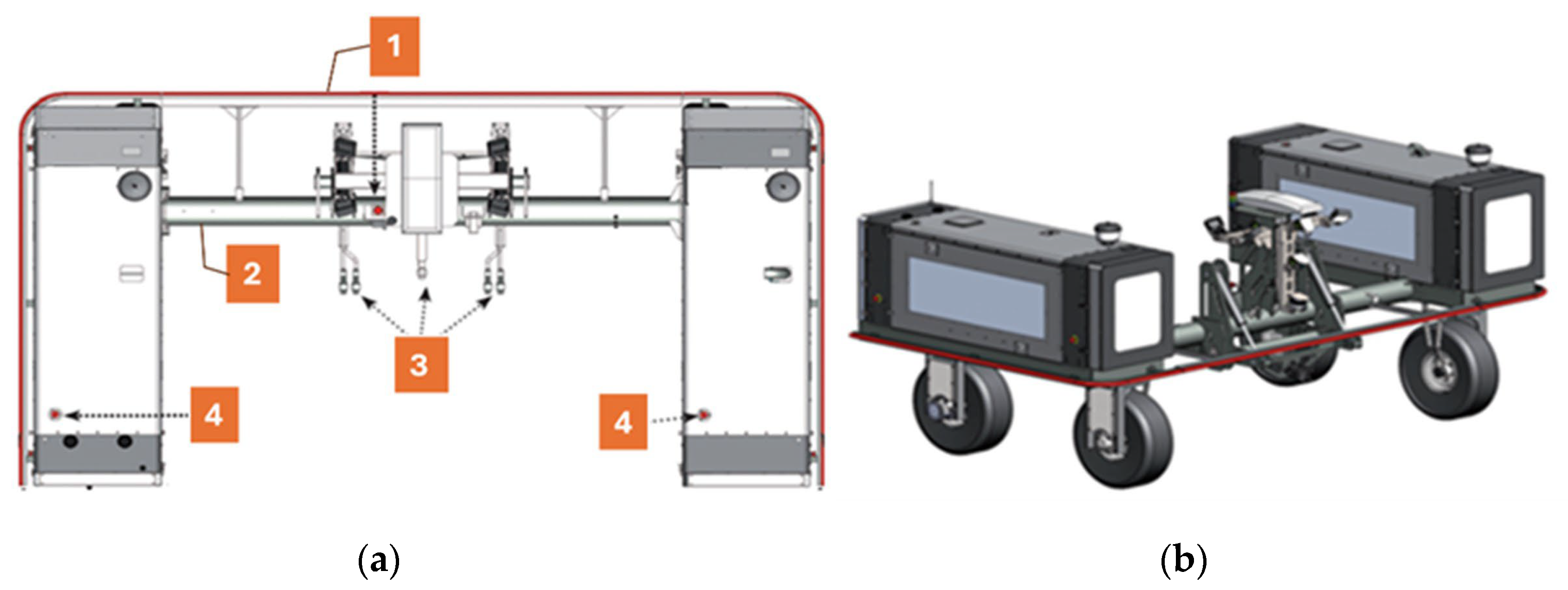
Machine learning and artificial intelligence problems can be grouped into three major types: supervised, unsupervised, and deep learning [14]. Supervised learning is recognized for utilizing labeled datasets, which are used to supervise or train algorithms that can precisely group information or forecast outcomes. The model can quantify its exactness and learn after some time thanks to labeled data sources and results [15]. Supervised learning can run into two kinds of problems: classification and regression. An algorithm is used in regression problems to train and validate regression models. Regression models include linear/nonlinear regression, support vector machine regression, regression trees and regression tree ensembles, gaussian process regression, and neural networks [16,17,18,19,20,21]. Figure 1 shows the steps that should be considered to resolve a supervised learning problem.

2.3. Robotic System

The robot displayed in Figure 2 exhibits a wide range of capabilities for performing agricultural tasks that are tailored to specific sites. These tasks encompass the preparation of seedbeds, seeding, hoeing, weeding, harrowing, soil sampling, spraying, and mowing. To cater to extensive fieldwork, the 150 D version of the robot has been purposefully designed, requiring PTO and external hydraulics for optimal functioning during seeding operations. It is equipped with two 56-kW Kubota diesel engines, generating a combined power output of up to 108 kW. The propulsion is driven by one engine, while the other engine powers the PTO and external hydraulic system. When operating in autonomous mode, the robot can achieve a maximum speed of 5 km/h, whereas in manual mode, it can reach up to 10 km/h. Weighing approximately 3100 kg, the robot efficiently executes 2-wheel steering using BKT AGRIMAXRT 657-320/65 R16 tires. To ensure precise navigation, the robot incorporates Real-Time Kinematic (RTK) GPS technology with a remarkable accuracy of 2 cm [4].

2.4. Data Acquisition

After each operation, all the information regarding the robot’s condition is collected from the sensors into two unique files: logging and location data. Logging and location files related to the 94 seeding operations of this robot were considered the dataset for this study. The logging file includes information such as speed, engine RPM, engine hydraulic pressure, steering hydraulic pressure, PTO power, fuel level, coolant temperature, time, etc. The location file includes information such as the coordinates of the robot, mode, status, time, etc. These files are obtained from the server in JSON format. To extract the necessary parameters from them, we must parse these files. The extracted data from the logging file was used for designing the first model based on the ASABE fuel consumption model. The robot’s movements were broken down into distinct job (time/distance) components using the information that was taken from the position file and examined. Figure 3 shows an example of the plotted coordinates of this robot.

The produced data can be combined to provide valuable information that can be used to assess performance metrics, identify turning patterns, and determine fieldwork patterns. Then, some parameters, such as total traveled distance, total time, automatic working distance, and automatic turning distance, can be calculated from each location file. Later, these parameters were used to develop the second model.

2.5. First Model (Based on ASABE Fuel Consumption Model)

In the first model, due to the fact that this robot has a diesel engine similar to a tractor, ASABE model was considered for estimating fuel consumption. The fuel consumption can be calculated at a given load with the engine running at a rated speed or less under ASABE standard D497.7 [22]:

$$X=P\times P_{rated}^{-1}$$

(1)

where X = fraction of equivalent PTO power available; P = equivalent PTO power required by the current operator (kW); P_rated = rated PTO power available (kW). The following formula can be used to determine the ratio of partial throttle engine speed to full throttle engine speed at operating load (N) and time (t):

$$N_t=n_{PTt}\times n_{FT}^{-1}$$

(2)

where $n_{PTt}$= partial throttle engine speed at time t (rpm); $n_{FT}$= full throttle engine speed (rpm). The partial throttle multiplier (PTM_t) in the SUTB approach (Shift Up Throttle Back: the SUTB methodology is used when less than full power is required) [8] can be calculated as follows:

$${PTM}_t=1-\left(N_t-1\right)\times (0.45X-0.877)$$

(3)

Specific fuel consumption volume (SFC_v, L/kW h) for diesel fuel can be calculated using the subsequent formula:

$${SFC}_{vt}=\left(0.0434+0.019 X^{-1}\right)\times {PTM}_t$$

(4)

The specific fuel consumption volume multiplied by the present power supply (PD, kW h) yields the fuel consumption (Q, L).

$$\mathrm{Q}={\sum }_t({SFC}_{vt}\times \mathrm{P}\mathrm{D})$$

(5)

2.6. Second Model (Based on Gaussian Process Regression Model)

In the second model, machine learning techniques were applied to predict fuel consumption based on the operational parameters of the robot (total traveled distance, total time, automatic working distance, and automatic turning distance). To accomplish this goal, we utilized the regression learner app (from the “Statistics and machine learning” toolbox) in MATLAB (version R2022b) [23] and conducted various predictive models. Out of all the models, gaussian process regression (GPR) exhibited the highest level of performance.

GPR models are nonparametric kernel-based probabilistic models. A generalized parity set (GP) is a collection of random variables with a joint Gaussian distribution for any finite number of them. Given n observations $(x_1,x_2,\dots ,x_n)$, the joint distribution of the random variables $f\left(x_1\right),f\left(x_2\right),\dots ,f\left(x_n\right)$ is Gaussian if $\left\{f\left(x\right),x\in {\mathbb{R}}^d\right\}$ is a GP. The covariance function $K(x,\acute{x})=Cov\left[f\right(x),f(\acute{x}\left)\right]=E\left[\right\{f\left(x\right)-m\left(x\right)\left\}\right\{f\left(\acute{x}\right)-m\left(\acute{x}\right)\left\}\right]$ and mean function $m\left(x\right)=E\left(f\right(x\left)\right)$ define a generalized gradient polynomial. Thus, the following can be used to model the response variable [24]:

$$y\left(x\right)=h{\left(x\right)}^T\beta +f\left(x\right)+\epsilon$$

(6)

where h(x) is a collection of basic functions that creates a new feature vector $h\left(x\right)$ in ${\mathbb{R}}^{\mathrm{p}}$ from the original feature vector $x$ in ${\mathbb{R}}^d$. $\beta$ is a vector of basis function coefficients that is $p-by-1$. $f\left(x\right)$ is a GP with zero mean and covariance function $K(x, \acute{x})$, $f\left(x\right) ~ GP(0,K(x,\acute{x}\left)\right)$ and $\epsilon$ is a Gaussian noise.

The main assumptions regarding the primary function to be represented inform the choice of the covariance (kernel) function $K(X,\acute{X})$ functional form. In this study, the Squared Exponential covariance function was employed in the GPR model. The expression for this kernel function is [24]:

$$K(X,\acute{X})={\sigma }^2{e}^{-\frac{{(x-\acute{x)}}^2}{{\lambda }^2}}$$

(7)

where $\lambda$ represents the length scales for each input (hyperparameters) and ${\sigma }^2$ is the variance. Regression fitting requires the hyperparameters of a chosen covariance function to be maximized in relation to experimental data in order to use gaussian processes.

2.6.1. Dataset Preparation

The information related to the total traveled distance, automatic working distance, automatic turning distance, and the total time of the operation was calculated and extracted from the 94 location files of the robot. To create a validation set, the dataset was subjected to k-fold cross-validation (K = 10). To test the model, 10 percent of the input data were considered a testing set. In this way, the data set is divided into 10% for validation, 10% for testing, and 80% for the training process. Cross-validation was selected as the validation scheme to protect the model against overfitting.

Data cleaning is a useful method that can identify and eliminate any potential errors or inconsistencies in the dataset and enhance the quality of the data. It includes reviewing, analyzing, detecting, modifying, or removing inappropriate data from a dataset to make it clean. There are some options, such as clean missing data, clean outlier data, normalize data, smooth data, and so on [25].

Table 1. Summary of input parameters for fuel consumption model.

	Minimum	Maximum	Mean	Median	Standard Deviation
fuelConsumption	0.101	13.96	3.015	0.998	4.372
traveledDist	9.941	9197	1863	335.1	2678
autoWorkDist	0	8805	1723	245.5	2579
autoTurnDist	0.101	1213	120.9	54.86	197.1
totalTime	71	8843	1831	646	2405

represents the main statistical properties related to the input parameters of the model.

For the input dataset, we considered cleaning outlier data by applying linear interpolation as the filling method and moving median as the detection method with a threshold factor equal to three. Figure 4 shows an example of applying a data cleaning technique to remove outliers from the input data.

2.6.2. Feature Selection and Hyperparameter Optimization

Feature selection and hyperparameter optimization are essential steps in building and improving machine learning models, as they can significantly impact a model’s performance and efficiency. Properly selecting relevant features and optimizing hyperparameters can lead to models that are more accurate, reliable, and computationally efficient [26,27].

Feature selection is the process of identifying and selecting the most relevant features from a dataset that will be used to train a machine learning model. This process is important because including irrelevant or redundant features can lead to overfitting, increase training time, and decrease the model’s overall performance [28]. There are various techniques for feature selection, such as Univariate Feature Selection, Recursive Feature Elimination, Principal Component Analysis (PCA), and Feature Importance. In this study, feature importance techniques were considered, which include machine learning algorithms that can be used to identify the most important features in a dataset.

Hyperparameters are model parameters that are set before the training process begins and cannot be learned from the data. Examples of hyperparameters include the learning rate, the number of trees in a random forest, or the depth of a decision tree. Hyperparameter optimization, also known as hyperparameter tuning, is the process of finding the best hyperparameters for a machine learning model to improve its performance [29]. There are various techniques for hyperparameter optimization, such as Grid Search, Random Search, Bayesian Optimization, and Genetic algorithms. Bayesian optimization is the method that is considered in this paper, and it uses probabilistic models to predict the performance of different hyperparameter configurations and selects the next set of hyperparameters to evaluate based on the model’s predictions [27].

2.7. Assess Model Performance

The trained model’s performance can be examined using the validation set. The validation set fitting performance (measured in RMSE) can be used as a criterion for selecting a model. The quality of fitting and performance of a model can be assessed using the following statistics: R-squared, the coefficient of determination, is typically more than zero and is always less than one. It contrasts the model that has been trained with the model whose response is constant and equal to the training response mean. The average squared difference between the estimated and actual values is known as the mean square error, or MSE. The response variable’s units correspond to the root mean squared error (RMSE), which is the root of MSE and is always positive. The mean absolute error (MAE) is less susceptible to outliers than the root mean square error (RMSE) and is always positive. R-squared values that are closer to 1 and lesser values for RMSE, MSE, and MAE indicate superior model performance. Furthermore, to determine whether there is a significant difference between the anticipated and observed values, a one-way analysis of variance (ANOVA) test was taken into consideration.

3. Results and Discussion

3.1. First Model (Based on ASABE Model)

By considering Equations (1)–(5), the values related to X (fraction of equivalent PTO power available), N (ratio of partial throttle engine speed to full throttle engine speed), PTM (partial throttle multiplier), SFC_v (specific fuel consumption volume), and Q (fuel consumption) for twenty logging files of this robot were calculated. Figure 5 shows the comparison of the predicted values for the fuel consumption of this robot by the ASABE model and the measured values.

Twenty random log files were selected, and the amount of fuel consumption based on the ASABE model was calculated and compared with the measured values. The results from

Table 2. Comparing the predicted fuel consumption values by ASABE model with the measured values.

N	Predicted (by ASABE)	Measured	Error
1	10.08	9.86	0.02
2	9.75	8.96	0.08
3	7.63	10.28	0.26
4	12.44	9.37	0.25
5	2.26	4.85	0.53
6	1.64	1.41	0.14
7	0.076	0.046	0.39
8	1.39	2.21	0.37
9	0.077	0.047	0.39
10	2.57	1.91	0.26
11	10.18	6.1	0.40
12	9.46	6.71	0.29
13	7.82	6.59	0.16
14	6.65	10	0.33
15	9.91	8.09	0.18
16	5.39	3.34	0.38
17	9.58	7.21	0.25
18	7.1	6.95	0.02
19	2.86	4.45	0.36
20	0.19	0.34	0.44

show that this model has an average error of 27.5% in predicting the value of fuel consumption for this robot. Table shows the values of measured and predicted fuel consumption.

Significant errors in predicting fuel consumption, particularly in cases 5, 7, and 11, can be attributed to various factors. These include the impact of field elevation, delays in sensor data recording, and inaccurate power delivery estimation.

3.2. Second Model (Predictive Model Using Machine Learning)

To develop a model for predicting the amount of fuel consumption based on the mentioned parameters, at the beginning, data cleaning methods were applied to improve the quality of the input dataset. Then, the cleaned data were considered input for the regression learner in MATLAB.

Table 3. The comparison of training results between applied predictive models.

Training Results
Model	RMSE (Validation)	R-Squared (Validation)	MSE (Validation)	MAE (Validation)	Prediction Speed (obs/s)	Training Time (s)
Ensemble	1.253	0.92	1.569	0.695	590	4.397
Fine Tree	1.378	0.90	1.899	0.671	3000	7.194
SVM	1.669	0.85	2.789	0.852	2100	1.742
GPR	1.659	0.85	2.751	0.814	1500	6.263
ANN	2.328	0.71	5.42	1.046	2100	19.20

shows the performance of various prediction models. The preliminary results show that the Ensemble model with hyperparameters of (minimum leaf size = 8, number of learners = 30, and learning rate = 0.1) has better performance than the other predictive models.

Table 4. The comparison of test results between applied predictive models.

Test Results
Model	RMSE (Test)	R-Squared (Test)	MSE (Test)	MAE (Test)
Ensemble	1.274	0.93	1.622	0.779
Fine Tree	0.986	0.96	0.973	0.539
SVM	0.79	0.97	0.624	0.508
GPR	0.998	0.96	0.995	0.644
ANN	1.256	0.94	1.577	0.631

shows the results of the test dataset. The raw data are set aside at 10% for validation, 10% for testing, and 80% for the training process. Cross-validation was selected as the validation scheme, which protects the model against overfitting.

Plots of the residuals (observed minus expected) versus the response variable’s predicted values were used to test for linear prediction bias and assess the acceptability of the model. Figure 6 represents the response plot and predicted vs. actual plot of the validation related to the Ensemble predictive model.

3.2.1. Feature Selection

The mentioned Ensemble prediction model considered four out of four features for the training. Feature selection is a technique that can be used for ranking the input features. There are a few algorithms that can be applied for feature selection, such as MRMR, F-Test, and RReliefF. Figure 7 demonstrates the feature importance scores using the mentioned ranking algorithms.

Table 5. The importance of features based on the applied ranking algorithms.

	MRMR	F-Test	RReliefF
totalTime	0.821	53.90	0.057
autoTurnDist	0.547	42.93	0.04
autoWorkDist	0.421	67.76	0.061
traveledDist	0.342	85.04	0.065

shows the importance of features based on the applied ranking algorithm. In the MRMR algorithm, “totalTime” has the highest score, and “traveledDist” has the lowest rank. In both F-Test and RReliefF, “traveledDist” has the higher score, and “autoTurnDist” has the lowest rank.

To investigate the effects of selecting features on the performance of the predictive models, each time one feature is going to remove and the results of predictive models is going to compare to see if we can obtain a better predictive model.

In the first step, the lowest-ranked feature is removed from the predictive models.

Table 6. Training results for predictive models with three features.

Training Results (Three Features)
Ranking Features Method	Best Predictive Model	RMSE (Validation)	R-Squared (Validation)	MSE (Validation)	MAE (Validation)	Prediction Speed (obs/s)	Training Time (s)
MRMR	Ensemble	1.589	0.87	2.528	0.884	860	5.688
F-Test	Fine Tree	1.379	0.90	1.901	0.702	5300	2.75
RReliefF	GPR	1.364	0.90	1.861	0.657	2700	9.457

shows the training results by considering three features for the predicting algorithms. Based on the results, the gaussian process regression (GPR) with coefficient determination (R² = 0.90), is the best model with considering three features.

Table 7. Test results for predictive models by applying feature ranking algorithm.

Test Results (Three Features)
Ranking Features Method	Best Predictive Model	RMSE (Test)	R-Squared (Test)	MSE (Test)	MAE (Test)
MRMR	Ensemble	0.806	0.96	0.65	0.519
F-Test	Fine Tree	1.772	0.82	3.141	0.937
RReliefF	GPR	0.868	0.96	0.753	0.51

shows the test results by considering three features and the Ensemble model with MRMR shows better performance with coefficient determination (R² = 0.96). Figure 8 shows the response plot and actual vs. predicted values for the validation set applying RReliefF algorithm for feature selection on GPR model.

Considering both training and test results for three features, it can be concluded that the gaussian process regression (GPR) with the coefficient determination of training and test equal to 0.90 and 0.96, respectively, has the best performance.

In this step, another lowest-ranked feature is removed from the predictive models.

Table 8. Training results for predictive models with two features.

Training Results (Two Features)
Ranking Features Method	Best Predictive Model	RMSE (Validation)	R-Squared (Validation)	MSE (Validation)	MAE (Validation)	Prediction Speed (obs/s)	Training Time (s)
MRMR	Fine Tree	1.396	0.90	1.949	0.74	6800	6.639
F-Test	SVM	1.457	0.89	2.122	0.775	5000	0.662
RReliefF	GPR	1.38	0.90	1.905	0.783	2800	5.92

and

Table 9. Test results for predictive models with two features.

Test Results (Two Features)
Ranking Features Method	Best Predictive Model	RMSE (Test)	R-Squared (Test)	MSE (Test)	MAE (Test)
MRMR	Fine Tree	1.268	0.92	1.608	0.901
F-Test	SVM	1.325	0.87	1.755	0.904
RReliefF	GPR	0.678	0.98	0.459	0.473

show the results of training and testing respectively after applying feature ranking algorithms. Based on the results, the GPR model with coefficient determination of training and test equal to 0.90 and 0.98, respectively, has the best performance. Figure 9 shows the response plot and actual vs. predicted values for the validation set in GPR model.

In the last step, another lowest-ranked feature is removed from the predicting models, and there is only one feature remaining.

Table 10. Training results for predictive models with one feature.

Training Results (One Feature)
Ranking Features Method	Best Predictive Model	RMSE (Validation)	R-Squared (Validation)	MSE (Validation)	MAE (Validation)	Prediction Speed (obs/s)	Training Time (s)
MRMR	Ensemble	1.274	0.91	1.622	0.693	1200	7.456
F-Test	GPR	1.169	0.93	1.368	0.762	3900	3.456
RReliefF	GPR	1.019	0.95	1.039	0.662	4500	2.639

and

Table 11. Test results for predictive models with one feature.

Test Results (One Feature)
Ranking Features Method	Best Predictive Model	RMSE (Test)	R-Squared (Test)	MSE (Test)	MAE (Test)
MRMR	Ensemble	1.298	0.95	1.685	0.929
F-Test	GPR	0.474	0.97	0.224	0.375
RReliefF	GPR	0.614	0.98	0.377	0.447

show the training and test results by applying different ranking feature methods. Based on the results, applying the RReliefF ranking algorithm in the GPR model has the best performance, with the coefficient determination of training and test equal to 0.95 and 0.98, respectively. Figure 10 shows the response plot and actual vs. predicted values for the validation set in the GPR model.

3.2.2. Hyperparameter Optimization

To improve the performance of predictive models, it is possible to optimize their internal parameters. The Regression Learner app tries various combinations of selected hyperparameter values by utilizing an optimization scheme that seeks to minimize the model mean squared error (MSE) and returns a model with the optimized hyperparameters.

For this purpose, four predictive models—Tree, SVM, GPR, Ensemble, and ANN—were selected. Bayesian optimization was considered the optimization scheme, with an acquisition function probability of improvement with 50 iterations.

Table 12. Training results by applying hyperparameter optimizer.

Training Results
Model	RMSE (Validation)	R-Squared (Validation)	MSE (Validation)	MAE (Validation)	Prediction Speed (obs/s)	Training Time (s)
Tree	1.271	0.91	1.616	0.732	1600	32.76
SVM	1.704	0.84	2.903	0.898	2100	61.94
GPR	1.107	0.93	1.224	0.583	1800	115.7
Ensemble	1.391	0.89	1.936	0.744	790	874
ANN	1.97	0.79	3.882	1.021	3300	473.7

and

Table 13. Test results by applying hyperparameter optimizer.

Test Results
Model	RMSE (Test)	R-Squared (Test)	MSE (Test)	MAE (Test)
Tree	0.308	1.00	0.095	0.242
SVM	1.819	0.88	3.308	0.961
GPR	0.277	1.00	0.077	0.216

show the results of applying hyperparameter optimization to the predictive models for training and test datasets. Figure 11 shows the response plot and actual vs. predicted values for the validation set in the GPR model by applying the hyperparameter optimizer.

The optimization results for gaussian process regression (GPR) for the hyperparameters Sigma, Basis function, and kernel function are 1.00444 × 10⁻⁴, constant, and Nonisotropic Exponential, respectively. Figure 12 shows the minimum MSE plot for the GPR predictive model.

The result of the one-way ANOVA test for the predicted values from the GPR model and observation is demonstrated in

Table 14. The result of one-way ANOVA test for all the GPR models.

ANOVA Table
Source	SS	df	MS	F	Prob > F
Columns	3.14	4	0.784	0.04	0.996
Error	7559.93	415	18.217
Total	7563.07	419

. The p-value of 0.9965 indicates that none of the predictive GPR models have means significantly different from the observation set. The calculated mean for each group (observation, GPR_1F, GPR_2F, GPR_3F, and GPR_opt) is 3.1506, 3.2496, 3.0882, 3.3309, and 3.1447, respectively. Based on the results, the optimized GPR shows better performance among other models.

A sensitivity analysis was also considered for the second model to better show the importance of input parameters in this model. Three different scenarios were considered to investigate the effect of changes on the input parameters of this model. Based on the values presented in Table 1, in each scenario, a maximum value was considered for the automatic working/turning distance. Here we assume that the traveled distance is the sum of the automatic working/turning distances.

Table 15. The result of sensitivity analysis for the input parameters of the second model.

Sensitivity Analysis
Input Parameters	Observed	1	2	3
Automatic working distance (m)	4770.7	8804.6	4770.7	8804.6
Automatic turning distance (m)	241.7	241.7	1213.3	1213.3
Traveled distance (m)	5012.5	9046.3	5984	10017.9
Total time (s)	6104	7005.6	6802.5	9704.5
Fuel consumption (L) (predicted by 2nd model)	5.3	6.4	5.9	8.5
Fuel consumption (L) (read)	5.1

shows the results of the sensitivity analysis for the second model.

Figure 13 shows that the traveled distance and the total time have a significant correlation with the fuel consumption of this robot.

When assessing the performance of prediction models, the R-squared number is frequently used to evaluate a model’s accuracy with respect to its predictions. Conversely, a model’s precision based on residual (error) analysis is often indicated by the RMSE. Because of this, it is better to consider multiple factors when evaluating or contrasting the overall effectiveness of prediction models. When modeling the fuel consumption based on operational parameters like total operational time, total traveled distance, automatic turning distance, and automatic working distance, the GPR model predicted with greater precision and accuracy, according to the goodness-of-fit in terms of R-Squared and RMSE corresponding to various predictive models—Tree, SVM, GPR, Ensemble, ANN, and so on. While large data sets are useful for creating effective models, statistically well-dispersed data in the input domain is a must for GPR models to work well [30,31].

Based on the results, the GPR model, by considering the number of preferred features, represents the best performance among other predictive models. The GPR model, by applying hyperparameter optimization with four features, represents the best performance with (R-Squared training = 0.93) and (R-Squared validation = 1.00). GPR model by applying the RReliefF algorithm with three features outperformed other models with (R-Squared training = 0.90) and (R-Squared validation = 0.96). Considering two features and applying the RReliefF algorithm again, the GPR model showed better performance with (R-Squared training = 0.90) and (R-Squared validation = 0.98). Finally, with one feature and considering the RReliefF algorithm for feature selection, GPR represents better results with (R-Squared training = 0.95) and (R-Squared validation = 0.98).

A sample field with a size equal to 0.56 ha (the sample field used in the first scenario [4]) was considered to compare the precision of the developed model in this study with the ASABE fuel consumption model. The measured fuel consumption for this field is 3.5 L. The total estimated fuel consumption for this field by the ASABE model is 4.48 L. The amount of predicted fuel consumption by using the developed model in this study is 4.19 L. The results show that the predicted fuel consumption by ASABE and the developed model in this study have 21.9% and 14% errors from the measured value, respectively. Therefore, the developed model in this study performs 36% better than the ASABE model in predicting the fuel consumption of this robot.

To provide a comprehensive comparison, some of the recent machine learning methods, such as gradient boosting, random forest, and XGBoost, were considered in this study to better evaluate and compare the performance of the proposed model.

In the first comparison, the gradient boosting regression method was considered. This estimator allows for the optimization of any differentiable loss function and constructs an additive model in a forward, step-by-step manner. A regression tree is fitted to the supplied loss function’s negative gradient at each step. The parameters of this regression model were set as follows (“loss function”: squared error, “learning rate”: 0.01, “number of estimators”: 500, “maximum depth”: 4, “minimum sample split”: 5). For data preprocessing, the train test split function was selected from the SKLEARN library with the parameters (X, Y, test size = 0.1, random state = 13), which splits the dataset into training and test datasets {X_train, X_test, y_train, y_test} with the size equal to {(83,4), (10,4), (83,1), (10,1)}, respectively. Then the gradient boosting regression model was initialized based on the mentioned parameters, and the model was fitted by considering (X_train, y_train). Based on the results, the values of mean squared error (MSE) and the coefficient of determination of the prediction (R²) for the test set are equal to 0.201 and 0.904, respectively. The values of MSE and R²for the GPR model with hyperparameter optimization (shown in Table 14) are 0.077 and 1.00. The comparison shows that the GPR model has better performance than the gradient-boosting regression model.

For the second comparison, the random forest regression model was considered. A random forest is a meta-estimator that employs averaging to increase prediction accuracy and manage over-fitting after fitting several classification decision trees on different dataset subsamples. The parameters of this regression model were set as follows: (“number of estimators”: 50, “criterion”: squared error, “maximum depth”: 2, “minimum sample split”: 2, “minimum samples leaf”: 1). For data preprocessing, the dataset was split in the same way as mentioned in the previous comparison. The random forest regressor model was initialized based on the mentioned parameters and fitted with X_train and y_train data. Based on the results, the values of mean squared error (MSE) and the coefficient of determination of the predictions (R²) for the test set in the random forest regressor are 0.15 and 0.928, respectively. The comparison shows that the GPR model has better performance than the random forest regression model.

The XGBoost regressor model, which offers parallel tree boosting (also known as GBDT or GBM) and can quickly and accurately address a variety of data science challenges, was taken into consideration for the final comparison. A useful gradient-boosting implementation for regression predictive modeling is called XGBoost. In order to create an XGBoost regression model, the hyperparameter values can be specified as follows: “number of estimators”: 1000, “maximum depth”: 7, “eta”: 0.1, “subsample”: 0.7, “colsample_bytree”: 0.8. For data preprocessing, the dataset was split into training and test datasets by applying the split function from the SKLEARN library. Then the model is fitted with the training dataset and can be used to make predictions for the test dataset. Based on the results, the values of the root mean square error (RMSE) for the test dataset and the coefficient of determination (R²) by applying the XGBoost regression model are 0.669 and 0.787, respectively. The comparison shows that the GPR model (Table 14) with RMSE (test) = 0.277 and R² (test) = 1.00 has better performance than the XGBoost regression model.

4. Conclusions

In this study, different machine learning techniques were applied to develop an effective model for estimating the fuel consumption of an agricultural robot. As the first model, the ASABE fuel consumption model was considered for predictions. The results show that the ASABE model has an average of 27.5% error in predicting the fuel consumption of the studied robot. The second model considers four operational features of the studied robot: total operational time, total traveled distance, automatic working distance, and automatic turning distance. The regression learner app from MATLAB software (version R2022b) was used for training and evaluating the performance of the developed models. Different methods, such as feature selection and hyperparameter optimization, were applied to improve the performance of the predictive models. The results show that the gaussian process regression (GPR) model has better performance in predicting the value of fuel consumption for this robot. The GPR model with four features, considering hyperparameter optimization, showed the best performance (R-Squared validation = 0.93, R-Squared test = 1.00) among other models. The comparison of the ASABE model and the developed model in this study reveals that the proposed model demonstrates a 36% increase in accuracy when predicting the fuel usage of this robot. Moreover, three different ML methods (gradient boosting, random forest, and XGBoost) were considered in this study and compared with the developed GPR model. The results show that the GPR model outperformed the mentioned models. The results of the one-way ANOVA test showed that the predicted values from GPR models and observation do not have significantly different means. Moreover, the results of the sensitivity analysis show that the traveled distance and the total time have a significant correlation with the fuel consumption of this robot.

References

1. Rahimi-Ajdadi, F.; Abbaspour-Gilandeh, Y. Artificial Neural Network and Stepwise Multiple Range Regression Methods for Prediction of Tractor Fuel Consumption. Measurement 2011, 44, 2104–2111. [Google Scholar] [CrossRef]
2. Tetteh, E.K.; Amankwa, M.O.; Yeboah, C. Emerging carbon abatement technologies to mitigate energy-carbon footprint—A review. Clean. Mater. 2021, 2, 100020. [Google Scholar] [CrossRef]
3. Mohammadi, A.; Rafiee, S.; Jafari, A.; Keyhani, A.; Mousavi-Avval, S.H.; Nonhebel, S. Energy use efficiency and greenhouse gas emissions of farming systems in north Iran. Renew. Sustain. Energy Rev. 2014, 30, 724–733. [Google Scholar] [CrossRef]
4. Vahdanjoo, M.; Gislum, R.; Aage Grøn Sørensen, C. Operational, Economic, and Environmental Assessment of an Agricultural Robot in Seeding and Weeding Operations. AgriEngineering 2023, 5, 299–324. [Google Scholar] [CrossRef]
5. Søgaard, H.T.; Aage Grøn Sørensen, C. A Model for Optimal Selection of Machinery Sizes within the Farm Machinery System. Biosyst. Eng. 2004, 1, 13–28. [Google Scholar] [CrossRef]
6. Yang, L.; Weize, T.; Weixin, Z.; Xinxin, W.; Zhibo, C.; Long, W.; Yuanyuan, X.; Caicong, W. Behavior Recognition and Fuel Consumption Prediction of Tractor Sowing Operations Using Smartphone. Int. J. Agric. Biol. Eng. 2022, 4, 154–162. [Google Scholar] [CrossRef]
7. Kichler, C.M.; Fulton, J.P.; Raper, R.L.; McDonald, T.P.; Zech, W.C. Effects of Transmission Gear Selection on Tractor Performance and Fuel Costs during Deep Tillage Operations. Soil Tillage Res. 2011, 2, 105–111. [Google Scholar] [CrossRef]
8. Kocher, M.F.; Smith, B.J.; Hoy, R.M.; Woldstad, J.C.; Pitla, S.K. Fuel Consumption Models for Tractor Test Reports. Trans. ASABE 2017, 3, 693–701. [Google Scholar] [CrossRef]
9. Kim, S.C.; Kim, K.U.; Kim, D.C. Prediction of Fuel Consumption of Agricultural Tractors. Appl. Eng. Agric. 2011, 5, 705–709. [Google Scholar] [CrossRef]
10. Grisso, R.D.; Kocher, M.F.; Vaughan, D.H. Predicting Tractor Fuel Consumption. Appl. Eng. Agric. 2004, 20, 553–561. [Google Scholar] [CrossRef]
11. Paraforos, D.S.; Griepentrog, H.W. Tractor fuel rate modeling and simulation using switching markov chains on can-bus data. IFAC-PapersOnLine 2019, 52, 379–384. [Google Scholar] [CrossRef]
12. Naik, V.S.; Raheman, H. Factors affecting fuel consumption of tractor operating active tillage implement and its prediction. Eng. Agric. Environ. Food 2019, 12, 548–555. [Google Scholar] [CrossRef]
13. Asinyetogha, H.I.; Raymond, A.E.; Silas, O.N. Predicting tractor fuel consumption during ridging on a sandy loam soil in a humid tropical climate. J. Eng. Technol. Res. 2019, 11, 29–40. [Google Scholar] [CrossRef]
14. Michael, W.B.; Azlinah, M.; Bee, W.Y. Supervised and Unsupervised Learning for Data Science, 1st ed.; Springer Nature Switzerland AG: Cham, Switzerland, 2020; pp. 3–21. ISBN 978-3-030-22474-5. [Google Scholar]
15. Dike, H.U.; Yimin, Z.; Kranthi, K.D.; Qingtian, W. Unsupervised Learning Based on Artificial Neural Network: A Review. In Proceedings of the IEEE International Conference on Cyborg and Bionic Systems (CBS), Shenzhen, China, 25–27 October 2018. [Google Scholar] [CrossRef]
16. Montgomery, D.C.; Peck, E.A.; Vining, G.G. Introduction to Linear Regression Analysis, 6th ed.; John Wiley & Sons, Inc.: Hoboken, NJ, USA, 2021. [Google Scholar]
17. Archontoulis, S.V.; Miguez, F.E. Nonlinear Regression Models and Applications in Agricultural Research. Agron. J. 2015, 107, 786–798. [Google Scholar] [CrossRef]
18. Zhang, F.; O’Donnell, L.J. Support Vector Regression. In Machine Learning; Academic Press: Cambridge, MA, USA, 2020; pp. 123–140. [Google Scholar] [CrossRef]
19. Breiman, L.; Friedman, J.H.; Olshen, R.A.; Stone, C.J. Classification and regression trees. WIREs Data Min. Knowl. Discov. 2017, 1, 14–23. [Google Scholar] [CrossRef]
20. Taki, M.; Rohani, A.; Soheili-Fard, F.; Abdeshahi, A. Assessment of Energy Consumption and Modeling of Output Energy for Wheat Production by Neural Network (MLP and RBF) and Gaussian Process Regression (GPR) Models. J. Clean. Prod. 2018, 172, 3028–3041. [Google Scholar] [CrossRef]
21. Bataineh, M.; Marler, T. Neural Network for Regression Problems with Reduced Training Sets. Neural Netw. 2017, 95, 1–9. [Google Scholar] [CrossRef]
22. American Society of Agricultural and Biological Engineers (ASABE). Agricultural Machinery Management Data—ASAE D497.7 MAR2011; ASABE: St. Joseph, MI, USA, 2011. [Google Scholar]
23. MathWorks. Statistics and Machine Learning Toolbox User’s Guide R2022b; MathWorks Inc.: Natick, MA, USA, 2022. [Google Scholar]
24. Rasmussen, C.E.; Williams, C.K. Gaussian Processes for Machine Learning; MIT Press: Cambridge, MA, USA, 2005. [Google Scholar] [CrossRef]
25. Whang, S.E.; Roh, Y.; Song, H.; Lee, J.G. Data Collection and Quality Challenges in Deep Learning: A Data-Centric AI Perspective. VLDB J. 2023, 32, 791–813. [Google Scholar] [CrossRef]
26. Martin, B.; Moosbauer, J.; Thomas, J.; Bischl, B. Multi-Objective Hyperparameter Tuning and Feature Selection Using Filter Ensembles. In Proceedings of the 2020 Genetic and Evolutionary Computation Conference, Cancún, Mexico, 8–12 July 2020. [Google Scholar] [CrossRef]
27. Yan, W.; Sherry Ni, X. A XGBOOST Risk Model via Feature Selection and Bayesian Hyper-Parameter Optimization. Int. J. Database Manag. Syst. 2019, 11, 1–17. [Google Scholar] [CrossRef]
28. Simon, F.; Wong, R.; Vasilakos, A.V. Accelerated PSO Swarm Search Feature Selection for Data Stream Mining Big Data. IEEE Trans. Serv. Comput. 2016, 9, 33–45. [Google Scholar] [CrossRef]
29. Li, Y.; Shami, A. On Hyperparameter Optimization of Machine Learning Algorithms: Theory and Practice. Neurocomputing 2020, 415, 295–316. [Google Scholar] [CrossRef]
30. Schulz, E.; Speekenbrink, M.; Krause, A. A tutorial on gaussian process regression: Modelling, exploring, and exploiting functions. J. Math. Psychol. 2018, 85, 1–16. [Google Scholar] [CrossRef]
31. Li, L.L.; Zhang, X.B.; Tseng, M.L.; Zhou, Y.T. Optimal scale gaussian process regression model in insulated gate bipolar transistor remaining life prediction. Appl. Soft Comput. 2019, 78, 261–273. [Google Scholar] [CrossRef]
Figure 1. The steps to resolve a supervised learning problem.
Agriengineering 06 00043 g001
Figure 2. Studied agricultural robot (version 150D). (a) Shows the top 2D view of the robot. Numbers 1 to 4 represent safety bumper, central boom, three-point-hitch, and emergency stop, respectively; (b) Shows the 3D view of the studied robot.
Agriengineering 06 00043 g002
Figure 3. Plotted coordinates of the robot based on different task (time/distance) elements. Green color represents manual driving; blue is for automatic and working mode; and white is for automatic and nonworking mode of the robot.
Agriengineering 06 00043 g003
Figure 4. Data cleaning process for the fuel consumption parameter.
Agriengineering 06 00043 g004
Figure 5. Comparison of predicted values for fuel consumption of this robot based on ASABE model with the measured values.
Agriengineering 06 00043 g005
Figure 6. The response plot and predicted vs. actual plot for the Ensemble model. In the left plot, the blue points are true values, the orange points are predicted values, and the orange lines are errors. In the right plot, the blue points are observations, and the black line is the prefect prediction.
Agriengineering 06 00043 g006
Figure 7. Feature ranking based on MRMR, F-Test, and RReliefF algorithms.
Agriengineering 06 00043 g007
Figure 8. The response plot and actual vs. predicted values for GPR model with three features.
Agriengineering 06 00043 g008
Figure 9. The response plot and actual vs. predicted values for GPR model with two features.
Agriengineering 06 00043 g009
Figure 10. The Response plot and Actual vs. Predicted values for GPR model with one feature.
Agriengineering 06 00043 g010
Figure 11. The response plot and actual vs. predicted values for GPR model with four features applying hyperparameter optimization.
Agriengineering 06 00043 g011
Figure 12. Minimum MSE plot for the GPR predictive model.
Agriengineering 06 00043 g012
Figure 13. The results of sensitivity analysis for the second model.
Agriengineering 06 00043 g013