
Multispectral Vegetation Indices and Machine Learning Approaches for Durum Wheat (Triticum durum Desf.) Yield Prediction across Different Varieties

 , ,
, ,  , , ,
, , , 
Abstract
:1. Introduction
2. Materials and Methods
2.1. Experimental Site
2.2. Experimental Design and Crop Management
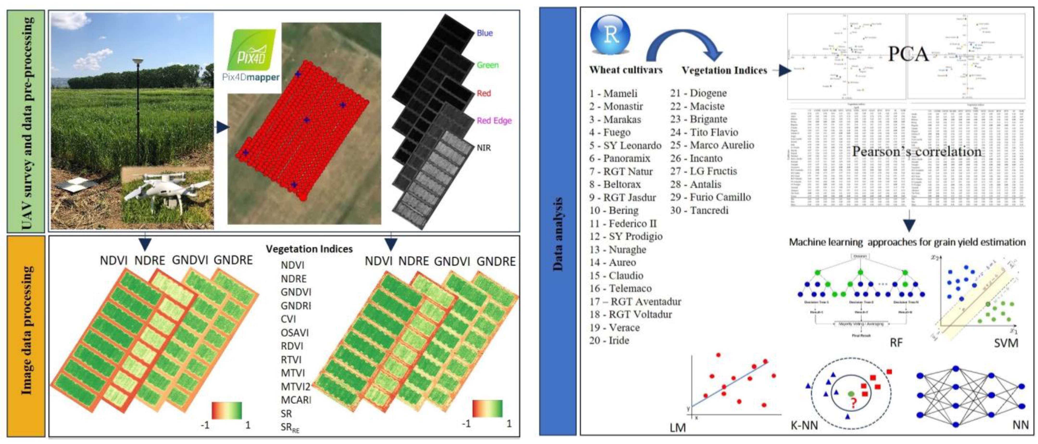
2.3. UAV Surveys and Image Processing
2.4. Statistics and Machine Learning (ML) Approaches
3. Results and Discussion
3.1. Indices (VIs) Responses of Durum Wheat Cultivars
3.2. Pearson’s Correlations Analysis between Grain Yield Data and Vegetation Indices (VIs) Responses
3.3. Machine Learning (ML) Approaches for Grain Yield Estimation
4. Conclusions
Author Contributions
Funding
Data Availability Statement
Acknowledgments
Conflicts of Interest
References
- Wiebe, K.; Robinson, S.; Cattaneo, A. Climate Change, Agriculture and Food Security. In Sustainable Food and Agriculture; Elsevier: Amsterdam, The Netherlands, 2019; pp. 55–74. [Google Scholar]
- Loboguerrero, A.; Campbell, B.; Cooper, P.; Hansen, J.; Rosenstock, T.; Wollenberg, E. Food and Earth Systems: Priorities for Climate Change Adaptation and Mitigation for Agriculture and Food Systems. Sustainability 2019, 11, 1372. [Google Scholar] [CrossRef]
- Tambe, E.B.; Anukwonke, C.C.; Mbuka-Nwosu, I.E.; Abazu, C.I. Changes in the Agriculture Sector That Are Essential to Mitigate and Adapt to Climate Changes. In Strategizing Agricultural Management for Climate Change Mitigation and Adaptation; Springer International Publishing: Cham, Switzerland, 2023; pp. 89–112. [Google Scholar]
- Durán-Sandoval, D.; Uleri, F.; Durán-Romero, G.; López, A.M. Food, Climate Change, and the Challenge of Innovation. Encyclopedia 2023, 3, 839–852. [Google Scholar] [CrossRef]
- Wesseler, J. The EU’s farm-to-fork strategy: An assessment from the perspective of agricultural economics. Appl. Econ. Perspect. Policy 2022, 44, 1826–1843. [Google Scholar] [CrossRef]
- Sissons, M. Durum Wheat Products—Recent Advances. Foods 2022, 11, 3660. [Google Scholar] [CrossRef]
- Xynias, I.N.; Mylonas, I.; Korpetis, E.G.; Ninou, E.; Tsaballa, A.; Avdikos, I.D.; Mavromatis, A.G. Durum Wheat Breeding in the Mediterranean Region: Current Status and Future Prospects. Agronomy 2020, 10, 432. [Google Scholar] [CrossRef]
- Carbone, A.; Henke, R. Recent trends in agri-food Made in Italy exports. Agric. Food Econ. 2023, 11, 32. [Google Scholar] [CrossRef]
- Recchia, L.; Cappelli, A.; Cini, E.; Garbati Pegna, F.; Boncinelli, P. Environmental Sustainability of Pasta Production Chains: An Integrated Approach for Comparing Local and Global Chains. Resources 2019, 8, 56. [Google Scholar] [CrossRef]
- Ciliberti, S.; Stanco, M.; Frascarelli, A.; Marotta, G.; Martino, G.; Nazzaro, C. Sustainability Strategies and Contractual Arrangements in the Italian Pasta Supply Chain: An Analysis under the Neo Institutional Economics Lens. Sustainability 2022, 14, 8542. [Google Scholar] [CrossRef]
- Abenavoli, L.; Milanovic, M.; Procopio, A.C.; Spampinato, G.; Maruca, G.; Perrino, E.V.; Mannino, G.C.; Fagoonee, S.; Luzza, F.; Musarella, C.M. Ancient wheats: Beneficial effects on insulin resistance. Minerva Med. 2021, 112, 641–650. [Google Scholar] [CrossRef]
- Perrino, E.V. Ancient and modern grains: Effects on human health: A first short review. Res. J. Ecol. Environ. Sci. 2022, 2, 21–25. [Google Scholar] [CrossRef]
- Santaga, F.S.; Agnelli, A.; Leccese, A.; Vizzari, M. Using Sentinel-2 for Simplifying Soil Sampling and Mapping: Two Case Studies in Umbria, Italy. Remote Sens. 2021, 13, 3379. [Google Scholar] [CrossRef]
- Santaga, F.S.; Benincasa, P.; Toscano, P.; Antognelli, S.; Ranieri, E.; Vizzari, M. Simplified and Advanced Sentinel-2-Based Precision Nitrogen Management of Wheat. Agronomy 2021, 11, 1156. [Google Scholar] [CrossRef]
- Messina, G.; Peña, J.M.; Vizzari, M.; Modica, G. A Comparison of UAV and Satellites Multispectral Imagery in Monitoring Onion Crop. An Application in the ‘Cipolla Rossa di Tropea’ (Italy). Remote Sens. 2020, 12, 3424. [Google Scholar] [CrossRef]
- Raeva, P.L.; Šedina, J.; Dlesk, A. Monitoring of crop fields using multispectral and thermal imagery from UAV. Eur. J. Remote Sens. 2019, 52, 192–201. [Google Scholar] [CrossRef]
- Peña, J.M.; Ostos-Garrido, F.J.; Torres-Sánchez, J.; Pistón, F.; de Castro, A.I. A UAV-based system for monitoring crop growth in wheat, barley and triticale phenotyping field trials. In Proceedings of the Precision Agriculture ’19; Wageningen Academic Publishers: Wageningen, The Netherlands, 2019; pp. 397–403. [Google Scholar]
- Messina, G.; Praticò, S.; Badagliacca, G.; Di Fazio, S.; Monti, M.; Modica, G. Monitoring Onion Crop “Cipolla Rossa di Tropea Calabria IGP” Growth and Yield Response to Varying Nitrogen Fertilizer Application Rates Using UAV Imagery. Drones 2021, 5, 61. [Google Scholar] [CrossRef]
- Modica, G.; Messina, G.; De Luca, G.; Fiozzo, V.; Praticò, S. Monitoring the vegetation vigor in heterogeneous citrus and olive orchards. A multiscale object-based approach to extract trees’ crowns from UAV multispectral imagery. Comput. Electron. Agric. 2020, 175, 105500. [Google Scholar] [CrossRef]
- Messina, G.; Fiozzo, V.; Praticò, S.; Siciliani, B.; Curcio, A.; Di Fazio, S.; Modica, G. Monitoring Onion Crops Using Multispectral Imagery from Unmanned Aerial Vehicle (UAV) BT—New Metropolitan Perspectives; Bevilacqua, C., Calabrò, F., Della Spina, L., Eds.; Springer International Publishing: Cham, Switerland, 2021; pp. 1640–1649. [Google Scholar]
- Marti, J.; Bort, J.; Slafer, G.A.; Araus, J.L. Can wheat yield be assessed by early measurements of Normalized Difference Vegetation Index? Ann. Appl. Biol. 2007, 150, 253–257. [Google Scholar] [CrossRef]
- Guo, C.; Tang, Y.; Lu, J.; Zhu, Y.; Cao, W.; Cheng, T.; Zhang, L.; Tian, Y. Predicting wheat productivity: Integrating time series of vegetation indices into crop modeling via sequential assimilation. Agric. For. Meteorol. 2019, 272–273, 69–80. [Google Scholar] [CrossRef]
- Casella, A.; Orden, L.; Pezzola, N.A.; Bellaccomo, C.; Winschel, C.I.; Caballero, G.R.; Delegido, J.; Gracia, L.M.N.; Verrelst, J. Analysis of Biophysical Variables in an Onion Crop (Allium cepa L.) with Nitrogen Fertilization by Sentinel-2 Observations. Agronomy 2022, 12, 1884. [Google Scholar] [CrossRef]
- Trevisan, L.R.; Brichi, L.; Gomes, T.M.; Rossi, F. Estimating Black Oat Biomass Using Digital Surface Models and a Vegetation Index Derived from RGB-Based Aerial Images. Remote Sens. 2023, 15, 1363. [Google Scholar] [CrossRef]
- Sharma, P.; Leigh, L.; Chang, J.; Maimaitijiang, M.; Caffé, M. Above-Ground Biomass Estimation in Oats Using UAV Remote Sensing and Machine Learning. Sensors 2022, 22, 601. [Google Scholar] [CrossRef] [PubMed]
- Wengert, M.; Piepho, H.-P.; Astor, T.; Graß, R.; Wijesingha, J.; Wachendorf, M. Assessing Spatial Variability of Barley Whole Crop Biomass Yield and Leaf Area Index in Silvoarable Agroforestry Systems Using UAV-Borne Remote Sensing. Remote Sens. 2021, 13, 2751. [Google Scholar] [CrossRef]
- Sharifi, A. Yield prediction with machine learning algorithms and satellite images. J. Sci. Food Agric. 2021, 101, 891–896. [Google Scholar] [CrossRef] [PubMed]
- Börjesson, T.; Wolters, S.; Söderström, M. Satellite-based modelling of protein content in winter wheat and malting barley. In Proceedings of the Precision Agriculture ’19; Wageningen Academic Publishers: Wageningen, The Netherlands, 2019; pp. 581–587. [Google Scholar]
- Chang, A.; Jung, J.; Yeom, J.; Maeda, M.M.; Landivar, J.A.; Enciso, J.M.; Avila, C.A.; Anciso, J.R. Unmanned Aircraft System- (UAS-) Based High-Throughput Phenotyping (HTP) for Tomato Yield Estimation. J. Sensors 2021, 2021, 8875606. [Google Scholar] [CrossRef]
- Mwinuka, P.R.; Mourice, S.K.; Mbungu, W.B.; Mbilinyi, B.P.; Tumbo, S.D.; Schmitter, P. UAV-based multispectral vegetation indices for assessing the interactive effects of water and nitrogen in irrigated horticultural crops production under tropical sub-humid conditions: A case of African eggplant. Agric. Water Manag. 2022, 266, 107516. [Google Scholar] [CrossRef]
- Tatsumi, K.; Igarashi, N.; Mengxue, X. Prediction of plant-level tomato biomass and yield using machine learning with unmanned aerial vehicle imagery. Plant Methods 2021, 17, 77. [Google Scholar] [CrossRef]
- Kyratzis, A.C.; Skarlatos, D.P.; Menexes, G.C.; Vamvakousis, V.F.; Katsiotis, A. Assessment of vegetation indices derived by UAV imagery for durum wheat phenotyping under a water limited and heat stressed Mediterranean environment. Front. Plant Sci. 2017, 8, 1114. [Google Scholar] [CrossRef]
- Gonzalez-Dugo, V.; Hernandez, P.; Solis, I.; Zarco-Tejada, P. Using High-Resolution Hyperspectral and Thermal Airborne Imagery to Assess Physiological Condition in the Context of Wheat Phenotyping. Remote Sens. 2015, 7, 13586–13605. [Google Scholar] [CrossRef]
- Fiorentini, M.; Schillaci, C.; Denora, M.; Zenobi, S.; Deligios, P.; Orsini, R.; Santilocchi, R.; Perniola, M.; Montanarella, L.; Ledda, L. A machine learning modeling framework for Triticum turgidum subsp. durum Desf. yield forecasting in Italy. Agron. J. 2022, in press. [Google Scholar] [CrossRef]
- Paudel, D.; Boogaard, H.; de Wit, A.; van der Velde, M.; Claverie, M.; Nisini, L.; Janssen, S.; Osinga, S.; Athanasiadis, I.N. Machine learning for regional crop yield forecasting in Europe. Field Crops Res. 2022, 276, 108377. [Google Scholar] [CrossRef]
- Soil Survey Staff. Keys to Soil Taxonomy. USDA-Natural Resources Conservation Service: Washington, DC, USA, 2014. [Google Scholar]
- Badagliacca, G.; Presti, E.L.; Ferrarini, A.; Fornasier, F.; Laudicina, V.A.; Monti, M.; Preiti, G. Early Effects of No-Till Use on Durum Wheat (Triticum durum Desf.): Productivity and Soil Functioning Vary between Two Contrasting Mediterranean Soils. Agronomy 2022, 12, 3136. [Google Scholar] [CrossRef]
- Modica, G.; De Luca, G.; Messina, G.; Praticò, S. Comparison and assessment of different object-based classifications using machine learning algorithms and UAVs multispectral imagery: A case study in a citrus orchard and an onion crop. Eur. J. Remote Sens. 2021, 54, 431–460. [Google Scholar] [CrossRef]
- Vincini, M.; Frazzi, E. Comparing narrow and broad-band vegetation indices to estimate leaf chlorophyll content in planophile crop canopies. Precis. Agric. 2011, 12, 334–344. [Google Scholar] [CrossRef]
- Cao, X.; Liu, Y.; Yu, R.; Han, D.; Su, B. A Comparison of UAV RGB and Multispectral Imaging in Phenotyping for Stay Green of Wheat Population. Remote Sens. 2021, 13, 5173. [Google Scholar] [CrossRef]
- Gitelson, A.A.; Kaufman, Y.J.; Merzlyak, M.N. Use of a green channel in remote sensing of global vegetation from EOS-MODIS. Remote Sens. Environ. 1996, 58, 289–298. [Google Scholar] [CrossRef]
- Haboudane, D.; Miller, J.R.; Pattey, E.; Zarco-Tejada, P.J.; Strachan, I.B. Hyperspectral vegetation indices and novel algorithms for predicting green LAI of crop canopies: Modeling and validation in the context of precision agriculture. Remote Sens. Environ. 2004, 90, 337–352. [Google Scholar] [CrossRef]
- Barnes, E.M.; Clarke, T.R.; Richards, S.E.; Colaizzi, P.D.; Haberland, J.; Kostrzewski, M.; Waller, P.; Choi, C.R.E.; Thompson, T.; Lascano, R.J.; et al. Coincident detection of crop water stress, nitrogen status and canopy density using ground based multispectral data. In Proceedings of the Fifth International Conference on Precision Agriculture, Bloomington, MN, USA, 16–19 July 2000; Volume 1619, p. 6. [Google Scholar]
- Rouse, J.W.; Haas, R.H.; Schell, J.A.; Deering, D.W. Monitoring vegetation systems in the Great Plains with ERTS. NASA Spec. Publ. 1974, 351, 309. [Google Scholar]
- Yue, J.; Yang, G.; Tian, Q.; Feng, H.; Xu, K.; Zhou, C. Estimate of winter-wheat above-ground biomass based on UAV ultrahigh-ground-resolution image textures and vegetation indices. ISPRS J. Photogramm. Remote Sens. 2019, 150, 226–244. [Google Scholar] [CrossRef]
- Roujean, J.-L.; Breon, F.-M. Estimating PAR absorbed by vegetation from bidirectional reflectance measurements. Remote Sens. Environ. 1995, 51, 375–384. [Google Scholar] [CrossRef]
- Chen, P.-F.; Nicolas, T.; Wang, J.-H.; Philippe, V.; Huang, W.-J.; Li, B.-G. New index for crop canopy fresh biomass estimation. Spectrosc. Spectr. Anal. 2010, 30, 512–517. [Google Scholar]
- Jordan, C.F. Derivation of Leaf-Area Index from Quality of Light on the Forest Floor. Ecology 1969, 50, 663–666. [Google Scholar] [CrossRef]
- Vogelmann, J.E.; Rock, B.N.; Moss, D.M. Red edge spectral measurements from sugar maple leaves. Int. J. Remote Sens. 1993, 14, 1563–1575. [Google Scholar] [CrossRef]
- De Mendiburu, F.; de Mendiburu, M.F. Package ‘agricolae’. R Packag. Version 2019, 1, 1–155. [Google Scholar]
- Husson, F.; Josse, J.; Le, S.; Mazet, J.; Husson, M.F. Package ‘factominer’. R Packag. 2016, 96, 698. [Google Scholar]
- Soetewey, A. Correlation Coefficient and Correlation Test in R-Stats and R. 2020, pp. 1–27. Available online: https://statsandr.com/blog/correlation-coefficient-and-correlation-test-in-r/ (accessed on 4 October 2023).
- Kuhn, M.; Wing, J.; Weston, S.; Williams, A. The caret package. Gene Expr. 2007, 28, 1–26. [Google Scholar]
- Hassan, M.A.; Yang, M.; Rasheed, A.; Yang, G.; Reynolds, M.; Xia, X.; Xiao, Y.; He, Z. A rapid monitoring of NDVI across the wheat growth cycle for grain yield prediction using a multi-spectral UAV platform. Plant Sci. 2019, 282, 95–103. [Google Scholar] [CrossRef] [PubMed]
- Marino, S.; Alvino, A. Agronomic traits analysis of ten winter wheat cultivars clustered by UAV-derived vegetation indices. Remote Sens. 2020, 12, 249. [Google Scholar] [CrossRef]
- Kefauver, S.C.; Vicente, R.; Vergara-Díaz, O.; Fernandez-Gallego, J.A.; Kerfal, S.; Lopez, A.; Melichar, J.P.E.; Serret Molins, M.D.; Araus, J.L. Comparative UAV and field phenotyping to assess yield and nitrogen use efficiency in hybrid and conventional barley. Front. Plant Sci. 2017, 8, 1733. [Google Scholar] [CrossRef]
- Adamsen, F.J.; Pinter, P.J.; Barnes, E.M.; LaMorte, R.L.; Wall, G.W.; Leavitt, S.W.; Kimball, B.A. Measuring Wheat Senescence with a Digital Camera. Crop Sci. 1999, 39, 719–724. [Google Scholar] [CrossRef]
- Morales, G.; Sheppard, J.W.; Logan, R.D.; Shaw, J.A. Hyperspectral Dimensionality Reduction Based on Inter-Band Redundancy Analysis and Greedy Spectral Selection. Remote Sens. 2021, 13, 3649. [Google Scholar] [CrossRef]
- Amankwah, A. Spatial Mutual Information Based Hyperspectral Band Selection for Classification. Sci. World J. 2015, 2015, 630918. [Google Scholar] [CrossRef] [PubMed]
- Marino, S.; Alvino, A. Detection of homogeneous wheat areas using multi-temporal UAS images and ground truth data analyzed by cluster analysis. Eur. J. Remote Sens. 2018, 51, 266–275. [Google Scholar] [CrossRef]
- Magney, T.S.; Eitel, J.U.H.; Huggins, D.R.; Vierling, L.A. Proximal NDVI derived phenology improves in-season predictions of wheat quantity and quality. Agric. For. Meteorol. 2016, 217, 46–60. [Google Scholar] [CrossRef]
- Fu, Z.; Jiang, J.; Gao, Y.; Krienke, B.; Wang, M.; Zhong, K.; Cao, Q.; Tian, Y.; Zhu, Y.; Cao, W.; et al. Wheat Growth Monitoring and Yield Estimation based on Multi-Rotor Unmanned Aerial Vehicle. Remote Sens. 2020, 12, 508. [Google Scholar] [CrossRef]
- Babar, M.A.; Reynolds, M.P.; van Ginkel, M.; Klatt, A.R.; Raun, W.R.; Stone, M.L. Spectral Reflectance Indices as a Potential Indirect Selection Criteria for Wheat Yield under Irrigation. Crop Sci. 2006, 46, 578–588. [Google Scholar] [CrossRef]
- Gutierrez, M.; Reynolds, M.P.; Raun, W.R.; Stone, M.L.; Klatt, A.R. Spectral Water Indices for Assessing Yield in Elite Bread Wheat Genotypes under Well-Irrigated, Water-Stressed, and High-Temperature Conditions. Crop Sci. 2010, 50, 197–214. [Google Scholar] [CrossRef]
- Xue, J.; Su, B. Significant Remote Sensing Vegetation Indices: A Review of Developments and Applications. J. Sensors 2017, 2017, 1353691. [Google Scholar] [CrossRef]
- Sellers, P.J. Canopy Reflectance, Photosynthesis, and Transpiration: II. The Role of Biophysics in the Linearity of Their Interdependence. Remote Sens. Environ. 1987, 21, 143–183. [Google Scholar] [CrossRef]
- Zhou, X.; Kono, Y.; Win, A.; Matsui, T.; Tanaka, T.S.T.T. Predicting within-field variability in grain yield and protein content of winter wheat using UAV-based multispectral imagery and machine learning approaches. Plant Prod. Sci. 2021, 24, 137–151. [Google Scholar] [CrossRef]
- Benincasa, P.; Antognelli, S.; Brunetti, L.; Fabbri, C.A.; Natale, A.; Sartoretti, V.; Modeo, G.; Guiducci, M.; Tei, F.; Vizzari, M. Reliability of ndvi derived by high resolution satellite and uav compared to in-field methods for the evaluation of early crop n status and grain yield in Wheat. Exp. Agric. 2018, 54, 604–622. [Google Scholar] [CrossRef]
- Yang, M.; Hassan, M.A.; Xu, K.; Zheng, C.; Rasheed, A.; Zhang, Y.; Jin, X.; Xia, X.; Xiao, Y.; He, Z. Assessment of Water and Nitrogen Use Efficiencies through UAV-Based Multispectral Phenotyping in Winter Wheat. Front. Plant Sci. 2020, 11, 927. [Google Scholar] [CrossRef] [PubMed]
- Sharma, L.; Bu, H.; Denton, A.; Franzen, D. Active-Optical Sensors Using Red NDVI Compared to Red Edge NDVI for Prediction of Corn Grain Yield in North Dakota, U.S.A. Sensors 2015, 15, 27832–27853. [Google Scholar] [CrossRef] [PubMed]
- Vincini, M.; Frazzi, E.; D’Alessio, P. A broad-band leaf chlorophyll vegetation index at the canopy scale. Precis. Agric. 2008, 9, 303–319. [Google Scholar] [CrossRef]
- Filippi, P.; Whelan, B.M.; Vervoort, R.W.; Bishop, T.F.A. Mid-season empirical cotton yield forecasts at fine resolutions using large yield mapping datasets and diverse spatial covariates. Agric. Syst. 2020, 184, 102894. [Google Scholar] [CrossRef]
- Yue, J.; Feng, H.; Yang, G.; Li, Z. A Comparison of Regression Techniques for Estimation of Above-Ground Winter Wheat Biomass Using Near-Surface Spectroscopy. Remote Sens. 2018, 10, 66. [Google Scholar] [CrossRef]
- Shendryk, Y.; Davy, R.; Thorburn, P. Integrating satellite imagery and environmental data to predict field-level cane and sugar yields in Australia using machine learning. Field Crops Res. 2021, 260, 107984. [Google Scholar] [CrossRef]
- Richetti, J.; Judge, J.; Boote, K.J.; Johann, J.A.; Uribe-Opazo, M.A.; Becker, W.R.; Paludo, A.; Silva, L.C.d.A. Using phenology-based enhanced vegetation index and machine learning for soybean yield estimation in Paraná State, Brazil. J. Appl. Remote Sens. 2018, 12, 026029. [Google Scholar] [CrossRef]
- Gómez, D.; Salvador, P.; Sanz, J.; Casanova, J.L. Modelling wheat yield with antecedent information, satellite and climate data using machine learning methods in Mexico. Agric. For. Meteorol. 2021, 300, 108317. [Google Scholar] [CrossRef]
- Leo, S.; De Antoni Migliorati, M.; Grace, P.R. Predicting within-field cotton yields using publicly available datasets and machine learning. Agron. J. 2021, 113, 1150–1163. [Google Scholar] [CrossRef]
- Bebie, M.; Cavalaris, C.; Kyparissis, A. Assessing Durum Wheat Yield through Sentinel-2 Imagery: A Machine Learning Approach. Remote Sens. 2022, 14, 3880. [Google Scholar] [CrossRef]
- Chergui, N. Durum wheat yield forecasting using machine learning. Artif. Intell. Agric. 2022, 6, 156–166. [Google Scholar] [CrossRef]
- Maltamo, M.; Kangas, A. Methods based on k -nearest neighbor regression in the prediction of basal area diameter distribution. Can. J. For. Res. 1998, 28, 1107–1115. [Google Scholar] [CrossRef]
- Montesinos López, O.A.; Montesinos López, A.; Crossa, J. Support Vector Machines and Support Vector Regression. In Multivariate Statistical Machine Learning Methods for Genomic Prediction; Springer International Publishing: Cham, Switzerland, 2022; pp. 337–378. [Google Scholar]
- Wang, L.; Zhou, X.; Zhu, X.; Dong, Z.; Guo, W. Estimation of biomass in wheat using random forest regression algorithm and remote sensing data. Crop J. 2016, 4, 212–219. [Google Scholar] [CrossRef]
- Zhu, W.; Li, S.; Zhang, X.; Li, Y.; Sun, Z. Estimation of winter wheat yield using optimal vegetation indices from unmanned aerial vehicle remote sensing. Trans. Chin. Soc. Agric. Eng. 2018, 34, 78–86. [Google Scholar]


| Band | Central Wavelength [nm] | Bandwidth [nm] |
|---|---|---|
| Blue | 450 | ±16 |
| Green | 560 | |
| Red | 650 | |
| Red Edge | 730 | |
| Near Infrared (NIR) | 840 | ±26 |
| Vegetation Index | Acronym | Formula | Reference |
|---|---|---|---|
| Chlorophyll Vegetation Index | CVI | [39] | |
| Green Normalised Difference Red Edge Index | GNDRE | [40] | |
| Green Normalised Difference Vegetation Index | GNDVI | [41] | |
| Modified Chlorophyll Absorption Ratio Index | MCARI2 | [42] | |
| Modified Triangular Vegetation Index | MTVI | ||
| Modified Triangular Vegetation Index 2 | MTVI2 | ||
| Normalised Difference Red Edge Index | NDRE | [43] | |
| Normalised Difference Vegetation Index | NDVI | [44] | |
| Optimised Soil Adjusted Vegetation Index | OSAVI | [45] | |
| Renormalised Difference Vegetation Index | RDVI | [46] | |
| Red Edge Triangulated Vegetation Index | RTVI | [47] | |
| Simple Ratio | SR | [48] | |
| Simple Ratio Red Edge | SRRE | [49] |
| Vegetation Indices—April | ||||||||||||||
|---|---|---|---|---|---|---|---|---|---|---|---|---|---|---|
| CVI | GNDRE | GNDVI | MCARI2 | MTVI | MTVI2 | NDRE | NDVI | OSAVI | RDVI | RTVI | SR | SR RE | ||
| Cultivars | Antalis | 2.04 c | 0.47 b | 0.69 b | 0.38 b | 0.19 c | 0.18 b | 0.33 c | 0.88 a | 0.46 c | 0.32 b | 5.34 a | 16.46 d | 2.02 e |
| Aureo | 1.94 e | 0.46 c | 0.68 b | 0.35 c | 0.21 a | 0.20 a | 0.33 c | 0.87 a | 0.49 a | 0.34 a | 5.85 a | 15.74 d | 2.01 e | |
| Beltorax | 1.84 g | 0.45 d | 0.66 c | 0.43 b | 0.19 d | 0.17 b | 0.30 d | 0.85 b | 0.44 c | 0.31 b | 4.74 b | 14.13 f | 1.89 g | |
| Bering | 1.87 f | 0.45 c | 0.66 c | 0.43 b | 0.19 d | 0.18 b | 0.31 d | 0.86 b | 0.45 c | 0.31 b | 4.78 b | 14.25 f | 1.90 g | |
| Brigante | 1.96 e | 0.47 b | 0.69 b | 0.36 c | 0.20 b | 0.19 a | 0.33 c | 0.88 a | 0.48 c | 0.33 a | 5.56 a | 16.43 d | 2.00 e | |
| Claudio | 1.87 f | 0.46 c | 0.67 b | 0.40 b | 0.19 c | 0.18 b | 0.31 c | 0.86 a | 0.46 c | 0.32 b | 5.00 b | 15.01 e | 1.92 g | |
| Diogene | 1.86 f | 0.46 b | 0.67 b | 0.41 b | 0.19 c | 0.18 b | 0.30 d | 0.86 b | 0.45 c | 0.31 b | 4.78 b | 15.05 e | 1.88 g | |
| Federico II | 2.05 c | 0.48 b | 0.70 a | 0.39 b | 0.18 e | 0.17 b | 0.34 c | 0.88 a | 0.45 c | 0.31 b | 5.12 b | 16.83 d | 2.03 d | |
| Fuego | 1.99 d | 0.47 b | 0.69 b | 0.37 c | 0.20 c | 0.19 b | 0.33 c | 0.88 a | 0.47 c | 0.32 b | 5.37 a | 16.55 d | 2.01 e | |
| Furio Camillo | 2.27 a | 0.48 a | 0.72 a | 0.35 c | 0.19 c | 0.18 b | 0.36 a | 0.89 a | 0.47 c | 0.32 b | 5.77 a | 18.40 a | 2.18 a | |
| Incanto | 1.80 h | 0.45 d | 0.66 c | 0.41 b | 0.20 b | 0.19 b | 0.3 d | 0.86 b | 0.46 c | 0.32 b | 4.94 b | 13.97 f | 1.86 h | |
| Iride | 2.00 d | 0.46 b | 0.69 b | 0.39 b | 0.19 c | 0.18 b | 0.33 c | 0.87 a | 0.46 c | 0.32 b | 5.30 a | 16.03 d | 2.01 e | |
| LG Fructis | 1.93 e | 0.47 b | 0.68 b | 0.36 c | 0.21 b | 0.19 a | 0.32 c | 0.87 a | 0.48 c | 0.33 a | 5.44 a | 15.79 d | 1.96 f | |
| Maciste | 2.10 b | 0.48 a | 0.71 a | 0.37 c | 0.19 d | 0.18 b | 0.34 c | 0.88 a | 0.46 c | 0.32 b | 5.32 a | 17.93 b | 2.07 c | |
| Mameli | 1.94 e | 0.46 c | 0.68 b | 0.41 b | 0.18 e | 0.17 c | 0.33 c | 0.87 a | 0.45 c | 0.31 b | 4.99 b | 15.75 d | 1.99 e | |
| Marakas | 1.87 f | 0.45 c | 0.67 b | 0.40 b | 0.19 c | 0.18 b | 0.32 c | 0.86 a | 0.45 c | 0.32 b | 5.02 b | 15.09 e | 1.94 f | |
| Marco Aurelio | 2.00 d | 0.47 b | 0.69 b | 0.38 b | 0.20 c | 0.18 b | 0.33 c | 0.87 a | 0.46 c | 0.32 b | 5.30 a | 16.17 d | 2.00 e | |
| Monastir | 1.97 d | 0.46 b | 0.68 b | 0.38 b | 0.20 b | 0.19 b | 0.32 c | 0.87 a | 0.47 c | 0.33 b | 5.38 a | 15.18 e | 1.96 f | |
| Nuraghe | 1.73 i | 0.44 d | 0.64 c | 0.42 b | 0.20 b | 0.19 b | 0.28 d | 0.85 c | 0.46 c | 0.32 b | 4.77 b | 13.30 g | 1.80 i | |
| Panoramix | 1.59 j | 0.42 e | 0.61 d | 0.48 a | 0.18 e | 0.17 c | 0.25 e | 0.83 d | 0.43 d | 0.30 c | 3.97 c | 11.86 g | 1.70 j | |
| RGT Aventadur | 2.03 c | 0.48 a | 0.71 a | 0.36 c | 0.19 c | 0.18 b | 0.35 c | 0.89 a | 0.47 c | 0.32 b | 5.49 a | 18.17 a | 2.08 c | |
| RGT Jasdur | 1.79 h | 0.46 b | 0.67 b | 0.37 c | 0.21 b | 0.19 a | 0.30 d | 0.87 a | 0.47 c | 0.33 b | 5.14 b | 15.61 e | 1.89 g | |
| RGT Natur | 1.93 e | 0.45 d | 0.66 b | 0.42 b | 0.19 d | 0.18 b | 0.31 c | 0.86 b | 0.45 c | 0.31 b | 4.93 b | 14.02 f | 1.93 f | |
| RGT Voltadur | 1.82 g | 0.45 d | 0.66 c | 0.40 b | 0.20 b | 0.19 b | 0.30 d | 0.86 b | 0.46 c | 0.32 b | 5.11 b | 14.26 f | 1.89 g | |
| SY Leonardo | 1.88 f | 0.46 b | 0.67 b | 0.39 b | 0.20 c | 0.18 b | 0.31 c | 0.87 a | 0.46 c | 0.32 b | 5.03 b | 15.35 e | 1.91 g | |
| SY Prodigio | 1.95 e | 0.48 b | 0.70 a | 0.35 c | 0.21 b | 0.19 a | 0.33 c | 0.88 a | 0.48 b | 0.33 a | 5.57 a | 17.17 c | 2.01 e | |
| Tancredi | 2.25 a | 0.48 b | 0.71 a | 0.37 c | 0.19 c | 0.18 b | 0.36 b | 0.88 a | 0.46 c | 0.32 b | 5.58 a | 17.22 c | 2.14 b | |
| Telemaco | 1.86 f | 0.46 c | 0.67 b | 0.41 b | 0.19 d | 0.18 b | 0.31 c | 0.86 b | 0.45 c | 0.31 b | 4.81 b | 15.00 e | 1.91 g | |
| Tito Flavio | 1.92 e | 0.46 b | 0.68 b | 0.39 b | 0.20 c | 0.18 b | 0.32 c | 0.87 a | 0.46 c | 0.32 b | 5.12 b | 15.56 e | 1.95 f | |
| Verace | 2.02 c | 0.46 b | 0.69 b | 0.39 b | 0.19 d | 0.18 b | 0.34 c | 0.87 a | 0.45 c | 0.32 b | 5.25 a | 16.20 d | 2.05 d | |
| Min | 1.59 | 0.42 | 0.61 | 0.35 | 0.18 | 0.17 | 0.25 | 0.83 | 0.43 | 0.30 | 3.97 | 11.86 | 1.70 | |
| Max | 2.27 | 0.48 | 0.72 | 0.48 | 0.21 | 0.20 | 0.36 | 0.89 | 0.49 | 0.34 | 5.85 | 18.40 | 2.18 | |
| Mean | 1.94 | 0.46 | 0.68 | 0.39 | 0.19 | 0.18 | 0.32 | 0.87 | 0.46 | 0.32 | 5.16 | 15.62 | 1.96 | |
| Δ VI | 0.68 | 0.06 | 0.11 | 0.13 | 0.03 | 0.03 | 0.11 | 0.06 | 0.06 | 0.04 | 1.88 | 6.54 | 0.48 | |
| p-value | <0.001 | <0.001 | <0.001 | 0.003 | 0.003 | 0.009 | <0.001 | <0.001 | 0.019 | 0.017 | 0.001 | <0.001 | <0.001 | |
| Vegetation Indices—May | ||||||||||||||
|---|---|---|---|---|---|---|---|---|---|---|---|---|---|---|
| CVI | GNDRE | GNDVI | MCARI2 | MTVI | MTVI2 | NDRE | NDVI | OSAVI | RDVI | RTVI | SR | SR RE | ||
| Cultivars | Antalis | 2.89 d | 0.48 c | 0.74 b | 0.17 a | 0.19 a | 0.18 a | 0.41 b | 0.81 c | 0.32 a | 0.47 a | 6.37 a | 17.25 c | 2.41 c |
| Aureo | 2.35 l | 0.45 f | 0.70 e | 0.18 a | 0.21 a | 0.20 a | 0.37 f | 0.79 f | 0.33 a | 0.48 a | 6.35 a | 14.87 f | 2.20 h | |
| Beltorax | 2.34 l | 0.45 f | 0.68 f | 0.16 a | 0.19 a | 0.18 a | 0.36 g | 0.77 g | 0.31 a | 0.45 a | 5.66 a | 14.89 f | 2.15 i | |
| Bering | 2.67 g | 0.47 d | 0.72 c | 0.16 a | 0.18 a | 0.17 a | 0.39 d | 0.80 e | 0.31 a | 0.45 a | 5.78 a | 16.02 d | 2.29 f | |
| Brigante | 2.76 e | 0.49 a | 0.73 b | 0.17 a | 0.19 a | 0.18 a | 0.39 c | 0.81 c | 0.32 a | 0.46 a | 6.13 a | 17.79 c | 2.33 d | |
| Claudio | 2.49 j | 0.46 e | 0.71 e | 0.18 a | 0.2 a | 0.19 a | 0.37 f | 0.79 e | 0.33 a | 0.47 a | 6.13 a | 15.25 e | 2.19 h | |
| Diogene | 2.73 e | 0.48 b | 0.73 b | 0.17 a | 0.19 a | 0.18 a | 0.40 c | 0.81 c | 0.32 a | 0.46 a | 6.03 a | 17.73 c | 2.34 d | |
| Federico II | 3.07 c | 0.49 a | 0.74 a | 0.15 a | 0.17 a | 0.16 a | 0.41 b | 0.81 c | 0.31 a | 0.44 a | 5.76 a | 17.16 c | 2.42 c | |
| Fuego | 2.52 i | 0.47 c | 0.72 c | 0.18 a | 0.20 a | 0.19 a | 0.39 c | 0.81 d | 0.33 a | 0.48 a | 6.36 a | 17.74 c | 2.32 e | |
| Furio Camillo | 3.14 b | 0.48 b | 0.75 a | 0.16 a | 0.18 a | 0.17 a | 0.43 a | 0.82 b | 0.32 a | 0.46 a | 6.36 a | 18.47 b | 2.56 a | |
| Incanto | 2.55 h | 0.46 e | 0.70 e | 0.16 a | 0.18 a | 0.17 a | 0.37 f | 0.79 f | 0.31 a | 0.45 a | 5.69 a | 15.06 e | 2.21 g | |
| Iride | 2.67 g | 0.47 c | 0.73 c | 0.17 a | 0.19 a | 0.18 a | 0.40 c | 0.81 d | 0.32 a | 0.46 a | 6.11 a | 16.96 d | 2.34 d | |
| LG Fructis | 2.68 g | 0.46 e | 0.72 d | 0.16 a | 0.18 a | 0.17 a | 0.39 c | 0.79 e | 0.31 a | 0.44 a | 5.77 a | 15.72 e | 2.31 e | |
| Maciste | 3.06 c | 0.49 a | 0.76 a | 0.17 a | 0.19 a | 0.18 a | 0.43 a | 0.83 a | 0.33 a | 0.47 a | 6.47 a | 19.30 a | 2.52 a | |
| Mameli | 2.63 g | 0.48 b | 0.74 a | 0.18 a | 0.20 a | 0.19 a | 0.41 b | 0.82 b | 0.34 a | 0.48 a | 6.66 a | 19.47 a | 2.43 c | |
| Marakas | 2.56 h | 0.47 d | 0.72 c | 0.18 a | 0.20 a | 0.19 a | 0.39 c | 0.80 d | 0.33 a | 0.47 a | 6.30 a | 16.53 d | 2.30 e | |
| Marco Aurelio | 2.77 e | 0.47 c | 0.72 d | 0.15 a | 0.18 a | 0.17 a | 0.39 d | 0.79 e | 0.31 a | 0.44 a | 5.67 a | 16.41 d | 2.30 e | |
| Monastir | 2.70 f | 0.47 c | 0.73 c | 0.17 a | 0.20 a | 0.18 a | 0.40 c | 0.81 d | 0.33 a | 0.47 a | 6.33 a | 16.54 d | 2.34 d | |
| Nuraghe | 2.37 k | 0.44 f | 0.68 f | 0.16 a | 0.19 a | 0.17 a | 0.35 h | 0.77 h | 0.31 a | 0.44 a | 5.44 a | 13.42 h | 2.09 j | |
| Panoramix | 2.18 m | 0.44 g | 0.68 f | 0.16 a | 0.19 a | 0.17 a | 0.34 i | 0.77 g | 0.31 a | 0.45 a | 5.30 a | 13.95 h | 2.06 k | |
| RGT Aventadur | 2.88 d | 0.48 b | 0.75 a | 0.17 a | 0.19 a | 0.18 a | 0.42 a | 0.82 b | 0.33 a | 0.47 a | 6.57 a | 18.59 b | 2.48 c | |
| RGT Jasdur | 2.41 j | 0.44 f | 0.67 f | 0.14 a | 0.17 a | 0.16 a | 0.34 i | 0.76 i | 0.30 a | 0.42 a | 5.01 a | 13.08 i | 2.07 k | |
| RGT Natur | 2.64 g | 0.45 f | 0.71 e | 0.16 a | 0.19 a | 0.18 a | 0.39 d | 0.79 e | 0.32 a | 0.46 a | 6.02 a | 14.60 g | 2.28 f | |
| RGT Voltadur | 2.47 j | 0.46 e | 0.71 e | 0.18 a | 0.20 a | 0.19 a | 0.38 e | 0.80 e | 0.33 a | 0.47 a | 6.31 a | 15.85 e | 2.25 g | |
| SY Leonardo | 2.54 h | 0.46 e | 0.71 e | 0.16 a | 0.19 a | 0.18 a | 0.38 e | 0.79 e | 0.32 a | 0.45 a | 5.87 a | 15.82 e | 2.25 g | |
| SY Prodigio | 2.44 j | 0.46 d | 0.72 d | 0.19 a | 0.21 a | 0.20 a | 0.38 d | 0.80 d | 0.34 a | 0.48 a | 6.48 a | 16.75 d | 2.27 f | |
| Tancredi | 3.19 a | 0.49 a | 0.75 a | 0.17 a | 0.19 a | 0.18 a | 0.43 a | 0.82 b | 0.32 a | 0.46 a | 6.50 a | 17.98 c | 2.54 a | |
| Telemaco | 2.65 g | 0.48 c | 0.73 c | 0.17 a | 0.2 a | 0.18 a | 0.39 c | 0.81 d | 0.33 a | 0.47 a | 6.21 a | 16.79 d | 2.31 e | |
| Tito Flavio | 2.46 j | 0.46 e | 0.71 e | 0.16 a | 0.18 a | 0.17 a | 0.37 f | 0.79 e | 0.31 a | 0.45 a | 5.62 a | 15.49 e | 2.20 h | |
| Verace | 2.69 f | 0.48 c | 0.74 a | 0.18 a | 0.20 a | 0.19 a | 0.42 b | 0.82 b | 0.34 a | 0.48 a | 6.73 a | 18.54 b | 2.44 c | |
| Min | 2.18 | 0.44 | 0.67 | 0.14 | 0.17 | 0.16 | 0.34 | 0.76 | 0.30 | 0.42 | 5.01 | 13.08 | 2.06 | |
| Max | 3.19 | 0.49 | 0.76 | 0.19 | 0.21 | 0.20 | 0.43 | 0.83 | 0.34 | 0.48 | 6.73 | 19.47 | 2.56 | |
| Mean | 2.65 | 0.47 | 0.72 | 0.17 | 0.19 | 0.18 | 0.39 | 0.80 | 0.32 | 0.46 | 6.07 | 16.47 | 2.31 | |
| Δ VI | 1.01 | 0.05 | 0.09 | 0.05 | 0.04 | 0.04 | 0.09 | 0.07 | 0.04 | 0.06 | 1.72 | 6.39 | 0.50 | |
| p-value | <0.001 | <0.001 | <0.001 | 0.310 | 0.120 | 0.220 | <0.001 | <0.001 | 0.471 | 0.416 | 0.525 | <0.001 | <0.001 | |
| Vegetation Indices—April | ||||||||||||||
|---|---|---|---|---|---|---|---|---|---|---|---|---|---|---|
| CVI | GNDRE | GNDVI | MCARI2 | MTVI | MTVI2 | NDRE | NDVI | OSAVI | RDVI | RTVI | SR | SR RE | ||
| Cultivars | Antalis | 0.74 | 0.97 | 0.94 | 0.63 | 0.15 | 0.23 | 0.82 | 0.98 | 0.51 | 0.51 | 0.41 | 0.90 | 0.76 |
| Aureo | 0.98 | 0.62 | 0.80 | 0.74 | 0.75 | 0.74 | 0.93 | 0.56 | 0.74 | 0.74 | 0.87 | 0.69 | 0.94 | |
| Beltorax | 0.19 | 0.49 | 0.36 | 0.56 | 0.80 | 0.76 | 0.08 | 0.38 | 0.66 | 0.67 | 0.45 | 0.19 | 0.02 | |
| Bering | 0.99 | 0.99 | 0.99 | 0.99 | 0.92 | 0.95 | 0.99 | 0.98 | 0.98 | 0.98 | 0.98 | 0.99 | 0.99 | |
| Brigante | 0.98 | 0.38 | 0.39 | 0.01 | 0.03 | 0.02 | 0.34 | 0.15 | 0.02 | 0.23 | 0.02 | 0.05 | 0.31 | |
| Claudio | 0.19 | 0.14 | 0.49 | 0.28 | 0.19 | 0.20 | 0.99 | 0.42 | 0.22 | 0.23 | 0.39 | 0.39 | 0.99 | |
| Diogene | 0.85 | 0.97 | 0.96 | 0.96 | 0.82 | 0.88 | 0.96 | 0.98 | 0.90 | 0.91 | 0.92 | 0.99 | 0.97 | |
| Federico II | 0.97 | 0.91 | 0.91 | 0.95 | 0.99 | 0.99 | 0.92 | 0.87 | 0.98 | 0.98 | 0.98 | 0.89 | 0.93 | |
| Fuego | 0.25 | 0.21 | 0.74 | 0.77 | 0.01 | 0.05 | 0.88 | 0.83 | 0.23 | 0.25 | 0.67 | 0.76 | 0.88 | |
| Furio Camillo | 0.61 | 0.26 | 0.31 | 0.33 | 0.88 | 0.70 | 0.35 | 0.15 | 0.53 | 0.50 | 0.54 | 0.17 | 0.35 | |
| Incanto | 0.76 | 0.96 | 0.95 | 0.57 | 0.20 | 0.26 | 0.95 | 0.66 | 0.35 | 0.37 | 0.60 | 0.82 | 0.95 | |
| Iride | 0.38 | 0.08 | 0.11 | 0.03 | 0.14 | 0.07 | 0.18 | 0.03 | 0.10 | 0.01 | 0.01 | 0.09 | 0.19 | |
| LG Fructis | 0.91 | 0.96 | 0.90 | 0.99 | 0.98 | 0.99 | 0.83 | 0.84 | 0.99 | 0.99 | 0.99 | 0.93 | 0.83 | |
| Maciste | 0.87 | 0.03 | 0.15 | 0.54 | 0.63 | 0.62 | 0.22 | 0.42 | 0.58 | 0.58 | 0.53 | 0.23 | 0.15 | |
| Mameli | 0.72 | 0.56 | 0.49 | 0.34 | 0.29 | 0.30 | 0.42 | 0.39 | 0.35 | 0.34 | 0.35 | 0.36 | 0.39 | |
| Marakas | 0.99 | 0.06 | 0.67 | 0.29 | 0.13 | 0.15 | 0.93 | 0.49 | 0.27 | 0.26 | 0.62 | 0.44 | 0.94 | |
| Marco Aurelio | 0.88 | 0.24 | 0.54 | 0.02 | 0.47 | 0.33 | 0.73 | 0.39 | 0.04 | 0.03 | 0.15 | 0.38 | 0.77 | |
| Monastir | 0.03 | 0.19 | 0.11 | 0.08 | 0.09 | 0.08 | 0.02 | 0.22 | 0.12 | 0.11 | 0.02 | 0.06 | 0.01 | |
| Nuraghe | 0.70 | 0.57 | 0.54 | 0.63 | 0.68 | 0.68 | 0.57 | 0.48 | 0.64 | 0.64 | 0.68 | 0.64 | 0.62 | |
| Panoramix | 0.27 | 0.98 | 0.76 | 0.92 | 0.99 | 0.99 | 0.58 | 0.92 | 0.98 | 0.97 | 0.73 | 0.81 | 0.57 | |
| RGT Aventadur | 0.72 | 0.99 | 0.99 | 0.99 | 0.98 | 0.98 | 0.99 | 0.91 | 0.99 | 0.99 | 0.97 | 0.99 | 0.97 | |
| RGT Jasdur | 0.21 | 0.84 | 0.75 | 0.77 | 0.77 | 0.76 | 0.43 | 0.98 | 0.78 | 0.78 | 0.62 | 0.66 | 0.34 | |
| RGT Natur | 0.02 | 0.03 | 0.04 | 0.24 | 0.83 | 0.76 | 0.02 | 0.05 | 0.53 | 0.51 | 0.14 | 0.02 | 0.01 | |
| RGT Voltadur | 0.30 | 0.88 | 0.78 | 0.80 | 0.80 | 0.80 | 0.58 | 0.89 | 0.81 | 0.81 | 0.66 | 0.80 | 0.53 | |
| SY Leonardo | 0.73 | 0.61 | 0.69 | 0.45 | 0.15 | 0.19 | 0.73 | 0.67 | 0.28 | 0.30 | 0.49 | 0.65 | 0.73 | |
| SY Prodigio | 0.92 | 0.81 | 0.99 | 0.89 | 0.05 | 0.05 | 0.95 | 0.97 | 0.33 | 0.37 | 0.71 | 0.99 | 0.92 | |
| Tancredi | 0.04 | 0.07 | 0.04 | 0.43 | 0.88 | 0.79 | 0.02 | 0.19 | 0.59 | 0.60 | 0.27 | 0.15 | 0.01 | |
| Telemaco | 0.03 | 0.05 | 0.13 | 0.06 | 0.01 | 0.02 | 0.25 | 0.18 | 0.04 | 0.04 | 0.08 | 0.17 | 0.23 | |
| Tito Flavio | 0.99 | 0.23 | 0.87 | 0.03 | 0.41 | 0.29 | 0.96 | 0.42 | 0.08 | 0.07 | 0.56 | 0.67 | 0.96 | |
| Verace | 0.93 | 0.92 | 0.99 | 0.99 | 0.99 | 0.99 | 0.98 | 0.99 | 0.99 | 0.99 | 0.99 | 0.99 | 0.99 | |
| Min | 0.02 | 0.03 | 0.04 | 0.01 | 0.01 | 0.02 | 0.02 | 0.03 | 0.02 | 0.01 | 0.01 | 0.02 | 0.01 | |
| Max | 0.99 | 0.99 | 0.99 | 0.99 | 0.99 | 0.99 | 0.99 | 0.99 | 0.99 | 0.99 | 0.99 | 0.99 | 0.99 | |
| Mean | 0.61 | 0.53 | 0.61 | 0.54 | 0.53 | 0.52 | 0.62 | 0.58 | 0.52 | 0.53 | 0.55 | 0.56 | 0.61 | |
| Vegetation Indices—May | ||||||||||||||
|---|---|---|---|---|---|---|---|---|---|---|---|---|---|---|
| CVI | GNDRE | GNDVI | MCARI2 | MTVI | MTVI2 | NDRE | NDVI | OSAVI | RDVI | RTVI | SR | SR RE | ||
| Cultivars | Antalis | 0.59 | 0.66 | 0.73 | 0.01 | 0.05 | 0.04 | 0.58 | 0.79 | 0.02 | 0.02 | 0.02 | 0.10 | 0.45 |
| Aureo | 0.03 | 0.81 | 0.22 | 0.39 | 0.48 | 0.45 | 0.04 | 0.32 | 0.46 | 0.45 | 0.45 | 0.08 | 0.07 | |
| Beltorax | 0.93 | 0.97 | 0.99 | 0.99 | 0.99 | 0.99 | 0.99 | 0.99 | 0.98 | 0.98 | 0.98 | 0.99 | 0.99 | |
| Bering | 0.76 | 0.09 | 0.62 | 0.12 | 0.06 | 0.08 | 0.84 | 0.39 | 0.11 | 0.12 | 0.12 | 0.44 | 0.87 | |
| Brigante | 0.99 | 0.75 | 0.63 | 0.97 | 0.95 | 0.97 | 0.02 | 0.59 | 0.99 | 0.99 | 0.99 | 0.02 | 0.21 | |
| Claudio | 0.38 | 0.01 | 0.02 | 0.03 | 0.04 | 0.01 | 0.03 | 0.04 | 0.02 | 0.01 | 0.04 | 0.05 | 0.03 | |
| Diogene | 0.52 | 0.49 | 0.62 | 0.26 | 0.12 | 0.18 | 0.79 | 0.64 | 0.21 | 0.24 | 0.24 | 0.92 | 0.84 | |
| Federico II | 0.99 | 0.98 | 0.12 | 0.34 | 0.37 | 0.37 | 0.24 | 0.69 | 0.37 | 0.38 | 0.38 | 0.13 | 0.34 | |
| Fuego | 0.02 | 0.89 | 0.58 | 0.45 | 0.37 | 0.41 | 0.33 | 0.53 | 0.43 | 0.42 | 0.42 | 0.93 | 0.33 | |
| Furio Camillo | 0.85 | 0.16 | 0.31 | 0.58 | 0.48 | 0.56 | 0.76 | 0.21 | 0.84 | 0.89 | 0.89 | 0.96 | 0.97 | |
| Incanto | 0.27 | 0.71 | 0.80 | 0.15 | 0.18 | 0.18 | 0.73 | 0.77 | 0.33 | 0.34 | 0.34 | 0.23 | 0.21 | |
| Iride | 0.90 | 0.68 | 0.99 | 0.50 | 0.48 | 0.55 | 0.45 | 0.96 | 0.89 | 0.92 | 0.92 | 0.11 | 0.35 | |
| LG Fructis | 0.99 | 0.91 | 0.88 | 0.90 | 0.85 | 0.88 | 0.80 | 0.86 | 0.92 | 0.92 | 0.92 | 0.80 | 0.79 | |
| Maciste | 0.57 | 0.87 | 0.64 | 0.01 | 0.03 | 0.02 | 0.29 | 0.68 | 0.18 | 0.02 | 0.04 | 0.02 | 0.45 | |
| Mameli | 0.56 | 0.48 | 0.64 | 0.97 | 0.99 | 0.98 | 0.78 | 0.63 | 0.92 | 0.92 | 0.92 | 0.65 | 0.78 | |
| Marakas | 0.99 | 0.90 | 0.99 | 0.67 | 0.60 | 0.65 | 0.95 | 0.99 | 0.77 | 0.77 | 0.77 | 0.98 | 0.94 | |
| Marco Aurelio | 0.61 | 0.56 | 0.77 | 0.99 | 0.99 | 0.99 | 0.97 | 0.75 | 0.99 | 0.98 | 0.98 | 0.98 | 0.99 | |
| Monastir | 0.34 | 0.10 | 0.69 | 0.62 | 0.58 | 0.59 | 0.98 | 0.97 | 0.55 | 0.55 | 0.55 | 0.96 | 0.71 | |
| Nuraghe | 0.04 | 0.89 | 0.99 | 0.99 | 0.99 | 0.99 | 0.98 | 0.98 | 0.99 | 0.99 | 0.99 | 0.99 | 0.93 | |
| Panoramix | 0.28 | 0.88 | 0.78 | 0.60 | 0.61 | 0.62 | 0.57 | 0.82 | 0.67 | 0.67 | 0.67 | 0.71 | 0.49 | |
| RGT Aventadur | 0.94 | 0.57 | 0.97 | 0.86 | 0.81 | 0.83 | 0.69 | 0.97 | 0.89 | 0.91 | 0.91 | 0.96 | 0.69 | |
| RGT Jasdur | 0.01 | 0.18 | 0.20 | 0.16 | 0.20 | 0.19 | 0.17 | 0.23 | 0.21 | 0.22 | 0.22 | 0.10 | 0.15 | |
| RGT Natur | 0.54 | 0.35 | 0.02 | 0.01 | 0.02 | 0.02 | 0.03 | 0.05 | 0.02 | 0.02 | 0.02 | 0.05 | 0.02 | |
| RGT Voltadur | 0.33 | 0.32 | 0.28 | 0.96 | 0.98 | 0.97 | 0.28 | 0.24 | 0.88 | 0.89 | 0.89 | 0.33 | 0.31 | |
| SY Leonardo | 0.02 | 0.37 | 0.02 | 0.17 | 0.01 | 0.03 | 0.02 | 0.14 | 0.01 | 0.02 | 0.01 | 0.90 | 0.02 | |
| SY Prodigio | 0.08 | 0.49 | 0.45 | 0.99 | 0.98 | 0.98 | 0.33 | 0.70 | 0.98 | 0.99 | 0.99 | 0.84 | 0.23 | |
| Tancredi | 0.03 | 0.92 | 0.35 | 0.66 | 0.73 | 0.72 | 0.21 | 0.56 | 0.72 | 0.72 | 0.72 | 0.49 | 0.25 | |
| Telemaco | 0.99 | 0.97 | 0.95 | 0.13 | 0.48 | 0.28 | 0.85 | 0.97 | 0.11 | 0.15 | 0.15 | 0.87 | 0.87 | |
| Tito Flavio | 0.97 | 0.66 | 0.45 | 0.46 | 0.42 | 0.42 | 0.44 | 0.35 | 0.40 | 0.40 | 0.40 | 0.52 | 0.51 | |
| Verace | 0.99 | 0.98 | 0.92 | 0.32 | 0.63 | 0.58 | 0.03 | 0.73 | 0.45 | 0.37 | 0.37 | 0.96 | 0.01 | |
| Min | 0.01 | 0.01 | 0.02 | 0.01 | 0.01 | 0.01 | 0.02 | 0.04 | 0.01 | 0.01 | 0.01 | 0.02 | 0.01 | |
| Max | 0.99 | 0.98 | 0.99 | 0.99 | 0.99 | 0.99 | 0.99 | 0.99 | 0.99 | 0.99 | 0.99 | 0.99 | 0.99 | |
| Mean | 0.55 | 0.62 | 0.59 | 0.51 | 0.52 | 0.52 | 0.51 | 0.62 | 0.54 | 0.54 | 0.54 | 0.57 | 0.49 | |
| April | May | ||||||
|---|---|---|---|---|---|---|---|
| R2 | RMSE | MAE | R2 | RMSE | MAE | ||
| Models | Linear model (LM) | 0.82 | 0.37 | 0.31 | 0.82 | 0.49 | 0.39 |
| Random forest (RF) | 0.88 | 0.18 | 0.16 | 0.84 | 0.36 | 0.27 | |
| Support Vector Machine (SVM) | 0.87 | 0.35 | 0.27 | 0.81 | 0.40 | 0.34 | |
| K-nearest neighbors (k-NN) | 0.86 | 0.27 | 0.23 | 0.85 | 0.44 | 0.36 | |
| Neural network (NN) | 0.71 | 1.00 | 1.90 | 0.68 | 1.94 | 1.90 | |
Disclaimer/Publisher’s Note: The statements, opinions and data contained in all publications are solely those of the individual author(s) and contributor(s) and not of MDPI and/or the editor(s). MDPI and/or the editor(s) disclaim responsibility for any injury to people or property resulting from any ideas, methods, instructions or products referred to in the content. |
© 2023 by the authors. Licensee MDPI, Basel, Switzerland. This article is an open access article distributed under the terms and conditions of the Creative Commons Attribution (CC BY) license (https://creativecommons.org/licenses/by/4.0/).
Share and Cite
Badagliacca, G.; Messina, G.; Praticò, S.; Lo Presti, E.; Preiti, G.; Monti, M.; Modica, G. Multispectral Vegetation Indices and Machine Learning Approaches for Durum Wheat (Triticum durum Desf.) Yield Prediction across Different Varieties. AgriEngineering 2023, 5, 2032-2048. https://doi.org/10.3390/agriengineering5040125
Badagliacca G, Messina G, Praticò S, Lo Presti E, Preiti G, Monti M, Modica G. Multispectral Vegetation Indices and Machine Learning Approaches for Durum Wheat (Triticum durum Desf.) Yield Prediction across Different Varieties. AgriEngineering. 2023; 5(4):2032-2048. https://doi.org/10.3390/agriengineering5040125
Chicago/Turabian StyleBadagliacca, Giuseppe, Gaetano Messina, Salvatore Praticò, Emilio Lo Presti, Giovanni Preiti, Michele Monti, and Giuseppe Modica. 2023. "Multispectral Vegetation Indices and Machine Learning Approaches for Durum Wheat (Triticum durum Desf.) Yield Prediction across Different Varieties" AgriEngineering 5, no. 4: 2032-2048. https://doi.org/10.3390/agriengineering5040125