An Artificial Intelligence and Industrial Internet of Things-Based Framework for Sustainable Hydropower Plant Operations

Abstract

Hydropower plays a crucial role in supplying electricity to developed nations and is projected to expand its capacity in various developing countries such as Sub-Saharan Africa, Argentina, Colombia, and Turkey. With the increasing demand for sustainable energy and the emphasis on reducing carbon emissions, the significance of hydropower plants is growing. Nevertheless, numerous challenges arise for these plants due to their aging infrastructure, impacting both their efficiency and structural stability. In order to tackle these issues, the present study has formulated a specialized real-time framework for identifying damage, with a particular focus on detecting corrosion in the conductors of generators within hydropower plants. It should be noted that corrosion processes can be highly complex and nonlinear, making it challenging to develop accurate physics-based models that capture all the nuances. Therefore, the proposed framework leverages autoencoder, an unsupervised, data-driven AI technology with the Mahalanobis distance, to capture the intricacies of corrosion and automate its detection. Rigorous testing shows that it can identify slight variations indicating conductor corrosion with over 80% sensitivity and a 5% false alarm rate for ‘medium’ to ‘high’ severity damage. By detecting and resolving corrosion early, the system reduces disruptions, streamlines maintenance, and mitigates unscheduled repairs’ negative effects on the environment. This enhances energy generation effectiveness, promotes hydroelectric facilities’ long-term viability, and fosters community prosperity.

1. Introduction

The United Nations’ 2030 agenda has set its sights on establishing sustainable infrastructure and industries, with a focus on promoting resource efficiency and eco-friendly technologies [1]. Hydropower presents itself as a versatile and cost-effective solution for generating low-carbon electricity, accounting for a significant 60% of all renewable energy sources and 16% of total electricity generation [2]. Not only do hydroelectric power plants actively contribute to reducing carbon emissions, but they also boast an impressively minimal carbon footprint. Moreover, they prove to be economically viable, with a long lifespan and relatively low operation and maintenance costs, typically amounting to around 2.5% of the overall plant cost [3]. However, while addressing climate change through transition methods remains a top priority, the stability of hydropower plant infrastructure presents challenges in achieving these goals. These challenges include conflicts over water resource management, such as those between farmers and industry, the impact of infrastructure on regional socio-economic activities, and the effects of operations on biodiversity.

The challenges faced by many existing hydroelectric power plant facilities are further exacerbated by their advanced age. For instance, approximately half of Greece’s hydroelectric power plants were built before 1975 [4], while the average hydroelectric facility in the United States has been operational for more than 64 years [5]. The aging infrastructures pose complexities that can lead to significant reductions in the power generation and overall efficiency of hydroelectric power plants. One significant issue that affects older hydroelectric power plants and hinders their effectiveness is the corrosion of conductors within the generator. This specific problem in energy production efficiency is linked to the concept of ‘current and voltage quality’, which refers to deviations of these measurements from their ideal sinusoidal form [6]. The corrosion of conductors can cause impedance variations, signal reflections, resistance alterations, and other irregularities that introduce noise into the measured signals (diverge from the sinusoidal form), thereby compromising their effectiveness in energy production.

To address this, a holistic platform has been proposed by many authors to promote sustainability in the hydropower sector, leveraging digital technology and organizational changes [7]. Previous studies have demonstrated the effective amalgamation of ad-hoc data fusion methods with cutting-edge artificial intelligence (AI) frameworks to support the execution of smart city strategies that prioritize sustainable industrial applications (e.g., [8,9,10]). Digital technology in hydropower operations improves information exchange among stakeholders and consolidates data into a centralized repository, enhancing sustainability and the management of prototype facilities. By adhering to robust sustainability standards, hydropower projects can gain investor confidence and public acceptance. In this direction, ref. [11] focused on advancing IoT sensor systems and digital solutions with AI and machine learning (ML).

The goal of this study was to develop a framework that can detect corrosion in aging hydroelectric power plant turbines, as there was a lack of such technology in the aged hydropower industry. We used an unsupervised damage detection framework that combined autoencoder [12] and Mahalanobis distance [13]. The autoencoder-based approach was suitable for anomaly detection as it is able to save through its weights the complex relationships to reconstruct the input as output of the healthy state, and once fed with a damaged (anomalous) state, it produces significant differences between the reconstructed and the actual input. The framework can be used in additional industries that use generators and are susceptible to corrosion. The main contributions of this study are:

• The framework allows for real-time analysis of data collected via electro generators in hydropower plants.
• The autoencoder architecture has been configured to accurately capture real-world datasets and their complex nature.
• Through evaluation using real-world datasets, it was shown that the framework is efficient and accurate.
• It can be integrated into aging hydroelectric power plants throughout their life cycle, improving management and maintenance practices.

The aforementioned framework’s ability to detect corrosion early optimizes maintenance and reduces energy leakage, leading to reduced downtime, improved maintenance schedules, minimized environmental impact, and optimized energy production from renewable sources.

In the subsequent sections, Section 2 discusses related work in corrosion detection and highlights the advantages of the current study. Section 3 analyzes the data acquisition system. The theoretical framework for damage detection is explained in Section 4, while Section 5 covers the experimental test case, including data quality and preprocessing procedures, descriptions of damage scenarios, and the training of the autoencoder. Section 6 presents a comprehensive overview of the damage detection results and a comparative analysis, and in Section 7, a discussion of the implementation on an actual power plant takes place. Finally, Section 8 concludes the study by summarizing the key findings.

2. Related Work

The current section composes a literature review on methods used for corrosion detection and related works that have used the autoencoder technology.

2.1. Related Work on Corrosion Detection

Corrosion poses a significant threat to the functionality of conductors and metallic structures, leading to potential catastrophic incidents. According to the World Corrosion Organization (WCO), the economic cost of corrosion-related problems amounts to a staggering 2.4 trillion USD annually, equivalent to 3% of the world’s gross domestic product (GDP) [14]. The engineering community has made remarkable advancements in addressing the detection and monitoring of corrosion in conductors and metallic structures. The existing literature outlines two primary categories of corrosion detection methods: physics-based and machine learning-based approaches. Physics-based methods primarily focus on identifying changes in physical and geometrical parameters such as impedance, resistance, and electromechanical noise generated by these changes. On the other hand, machine learning-based methods aim to classify data into damaged or healthy groups and determine the structural health state. Various physics-based methods have been developed for corrosion detection, including direct approaches like corrosion coupons, electrical resistance, ultrasonic, and acoustic emission, as well as electromechanical approaches like harmonic distortion analysis, electromechanical noise, and linear polarization resistance [3,15]. Indirect approaches were also extensively discussed in [15]. While these methods have proven effective and offer advantages depending on the specific application, they encounter significant challenges when applied to conductors within a generator due to the limited space and the requirement to interrupt its operation. In contrast, time domain reflectometry (TDR) [16] emerges as a cutting-edge method for corrosion detection in conductors without the need for operational interruption. TDR involves transmitting a pulse or step signal along a conductor and measuring the time it takes for the signal to be reflected back.

Recent studies (e.g., [17]) have revealed that machine learning-based techniques, such as artificial neural networks (ANN), random forest (RF), and support vector machines (SVM), demonstrate impressive diagnostic accuracy. These techniques have gained popularity due to advancements in data acquisition, saving, and transport systems. However, they primarily operate within a supervised framework, which poses challenges when accessing signals or images from compromised structures that are not easily accessible. In particular, deep learning ANN models that rely on images [18] face practical difficulties in confined spaces like the inner sections of generators. Moreover, hydropower plants experience significant variations in environmental conditions (temperature, humidity) and operational conditions (loads) throughout their operational phases. Data logs that capture these changes are often unavailable or hard to obtain. These variations can potentially overlap with deviations caused by corrosion (damage) in the collected data, thereby compromising the detection process. Therefore, it is crucial to develop a robust and sophisticated framework that can effectively differentiate between these types of deviations and accurately detect corrosion in hydropower plants.

Corrosion processes can be highly complex and nonlinear, making it challenging to develop accurate physics-based models that capture all the nuances. Data-based methods, particularly machine learning algorithms, can handle complex relationships and patterns in data without the need for explicit knowledge of underlying physical processes. This adaptability is particularly useful when dealing with real-world variability. Additionally, physics-based models may struggle with uncertainties in material properties, environmental conditions, and other factors affecting corrosion. Data-based methods can implicitly account for uncertainties by learning patterns and relationships from data, making them robust in the face of incomplete or uncertain information. The data-based methods reviewed often require measurements taken in damaged conditions. However, obtaining such measurements may not always be feasible. Hence, it becomes imperative to adopt an anomaly detection approach to address this limitation.

2.2. Related Work for Autoencoders

The autoencoder is a widely recognized AI technique for detecting anomalies. It has been successfully applied in various domains, such as fault detection in wind turbines [19], monitoring hydroelectric power plants using shallow autoencoders coupled with hotelling control charts [20], detecting anomalies in surveillance videos [21], and identifying anomalies in MRI images [22]. The autoencoder is known for its versatility and reliability, especially when combined with a robust statistical distance. Despite the availability of numerous anomaly detection methods based on AI or machine learning (ML) technologies, one of the key advantages of the autoencoder is its ability to quantify anomalies and track their progression, meaning that as the damage progresses and its severity rises (i.e., corrosion area), the Mahalanobis distance computed increases as the damaged state of the conductor further diverges from the healthy state. Constantly monitoring the distance increase offers supervision of the damage progression as well. Therefore, it was selected as the anomaly detection technology for the current study, considering all the benefits it offers.

The engineering community primarily focuses on condition monitoring at hydroelectric power plants to prevent catastrophic faults. However, this often overlooks the decrease in energy production efficiency caused by corrosion in conductors. This study aims to propose an AI-based, real-time, unsupervised corrosion monitoring framework and system. It can be retrofitted in older hydroelectric power plants to detect corrosion early, improving the quality of electric power and energy efficiency.

3. The Data Acquisition System Description

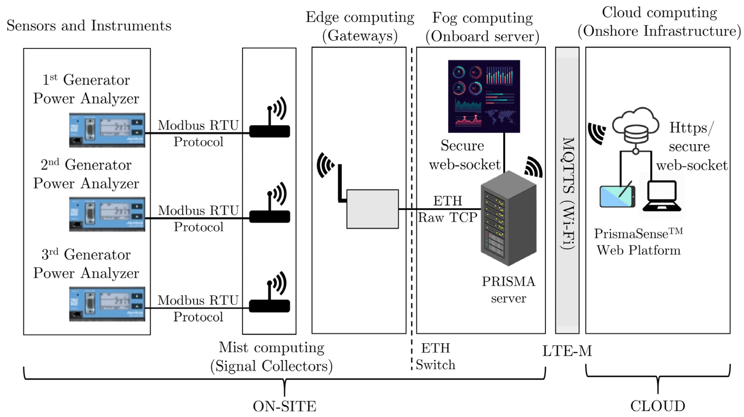
In the process of data-driven damage diagnostics, the initial step involves obtaining and storing crucial data. There are two categories of data used for health and condition-based maintenance: event data and condition data. Event data encompasses historical information regarding faults, breakdowns, repairs, causes, actions taken, and conditions. On the other hand, condition data consists of measurements pertaining to the health status of the asset, such as vibration, oil analysis, temperature, pressure, and moisture/humidity. The current study utilized the PrismaSense™ [23] data acquisition system/platform. This system incorporates a hybrid data fusion architecture, which facilitates the distribution of processing power and storage capacity across different levels. The data fusion architecture is visually depicted in Figure 1.

A secure wired network was established within the power plant to transmit measurements wirelessly to the gateway. This network consisted of signal collectors and power analyzers communicating with the Modbus RTU protocol. The wireless transmission relied on the IEEE 802.15.4 Zigbee encoding wireless protocol, with additional layers and data formats to meet the requirements of the hydroelectric power plant environment and enhance the network quality of service. The gateways were connected to the onboard Prisma server via ethernet and raw TCP protocols. The data was then transferred and secured using WebSocket security protocols to ensure its safety. The cloud server acquired the data via Wi-Fi for further computing processes as well as to be visualized to gain a better understanding and derive insights.

The power analyzer measured the current and voltage of the three-phase 4-conductors (line-to-neutral and line-to-line) system with a resolution of 10 mA and 0.01 V, respectively, over a time period of 12 sampling periods. The sampling frequency of these values was 20 kHz. The effective values and additional physical quantities were computed over the 12 sampling periods time window every 5 min. The rate at which values are computed may be changed by the user.

It should be noted that Prisma Sense was already mounted in an aged power plant and therefore the data was available for analysis. Therefore, the analysis preceded the selection of the data acquisition system.

4. Damage Detection Methodology

The framework was built upon the well-established autoencoder, a neural network that was designed to reconstruct its input as the output. The autoencoder was trained using only healthy data and operated in an unsupervised manner. During the Training Phase (TP), the autoencoder captured and retained the effects of environmental and operating conditions (EOCs) in its weights and biases. When a new signal set was obtained, with an unknown health state, a feature vector was created and fed into the autoencoder. The autoencoder then reconstructed the input as output, and any significant differences beyond a user-defined threshold indicated potential damage. To measure these differences, the framework utilized the Mahalanobis distance, which took into account the variability of the training data, thereby improving the overall robustness. Once the autoencoder is trained and the threshold is set, it can operate automatically and in real-time (online).

The damage detection framework consisted of two distinct phases: the Training Phase (TP) and the Inspection Phase (IP). The Training Phase involved the initial configuration of hyperparameters (such as feature samples m), training of the autoencoder model, and computation of the Mahalanobis sample mean vector and sample covariance matrix. These actions can be performed offline to establish a reference baseline for damage detection. On the other hand, the Inspection Phase pertains to the active deployment of the model for real-time data acquisition, feature construction, and assessment of deviations in the new feature vector from the reference baseline. This allows for automated decision-making. It is important to note that the Training Phase took place after the data had been acquired and preprocessed. It was subsequently divided into the following five tasks:

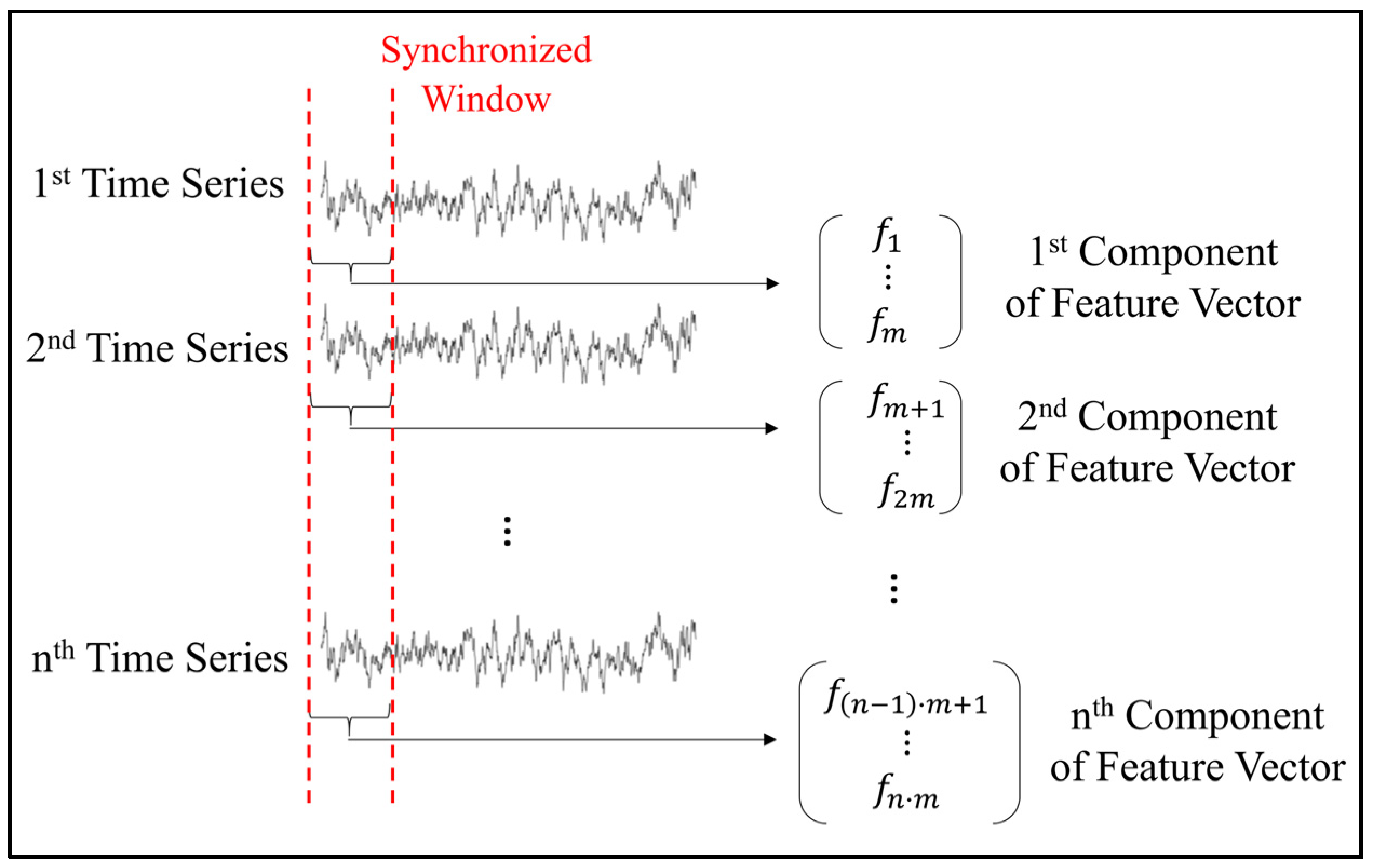
TP Task 1: Feature construction. The sensitive-to-damage features were created using the preprocessed time series data. Each time series represented a different physical measurement, such as phase current or phase voltage. From each distinct time series, a set of m samples was systematically chosen using a synchronized window. These samples were then arranged into a sequential vector called a feature vector, as shown in Figure 2. The feature vector consisted of n components derived from each distinct time series.

To maintain coherence, the window slides to the right without any overlap. This meant that each feature vector contained unique samples from the n-time series. If the last samples of a time series did not complete an m-tuple, they were omitted and did not contribute to the feature vector. As a result, the dimensionality of the multidimensional feature vectors was nxm.

In the current study, only 6 distinct time series were used, and a window of 12 samples was selected. This led to a feature vector dimensionality of 72.

TP Task 2: Configuring the autoencoder. The dimensions of the input and output layers in the autoencoder were determined by the feature vectors. Typically, two layers were chosen between the input layer and the bottleneck layer, as well as between the bottleneck layer, and the output layer. The user has the ability to select the number of neurons in the intermediate layers and the bottleneck layer, following a specific rule. They can also choose the activation functions for these layers, except for the output layer which is preselected as a rectified linear unit (ReLU) function. The rule for the number of neurons was as follows: the number of neurons should decrease from the input layer to the bottleneck layer and then increase from the bottleneck layer to the output layer. A detailed description of the chosen autoencoder can be found in the relevant subsection.

TP Task 3: Training the autoencoder. The configured autoencoder model was trained and validated.

TP Task 4: Mahalanobis distance sample mean vector and sample covariance computation. The Mahalanobis distance measured the dissimilarity between the input and output by calculating the reconstruction error. This error was obtained from the error vector, which represented the element-wise difference between the input and output. It is important to note that the error vector had smaller dimensions (k) compared to the feature vector (nxm) because values nullified in the output due to the ReLU activation function were not included in the error vector. The Mahalanobis distance incorporated two specific hyperparameters: the sample mean and the sample covariance matrix. These hyperparameters were computed as the average value and covariance matrix of the available k-dimensional error vectors from the training set, thereby maintaining the unsupervised nature of the framework.

TP Task 5: User-defined threshold. The user can establish the threshold for the decision-making process either through intuitive judgment or by using statistical tools. Statistical tools can make use of the Mahalanobis distances obtained during the TP.

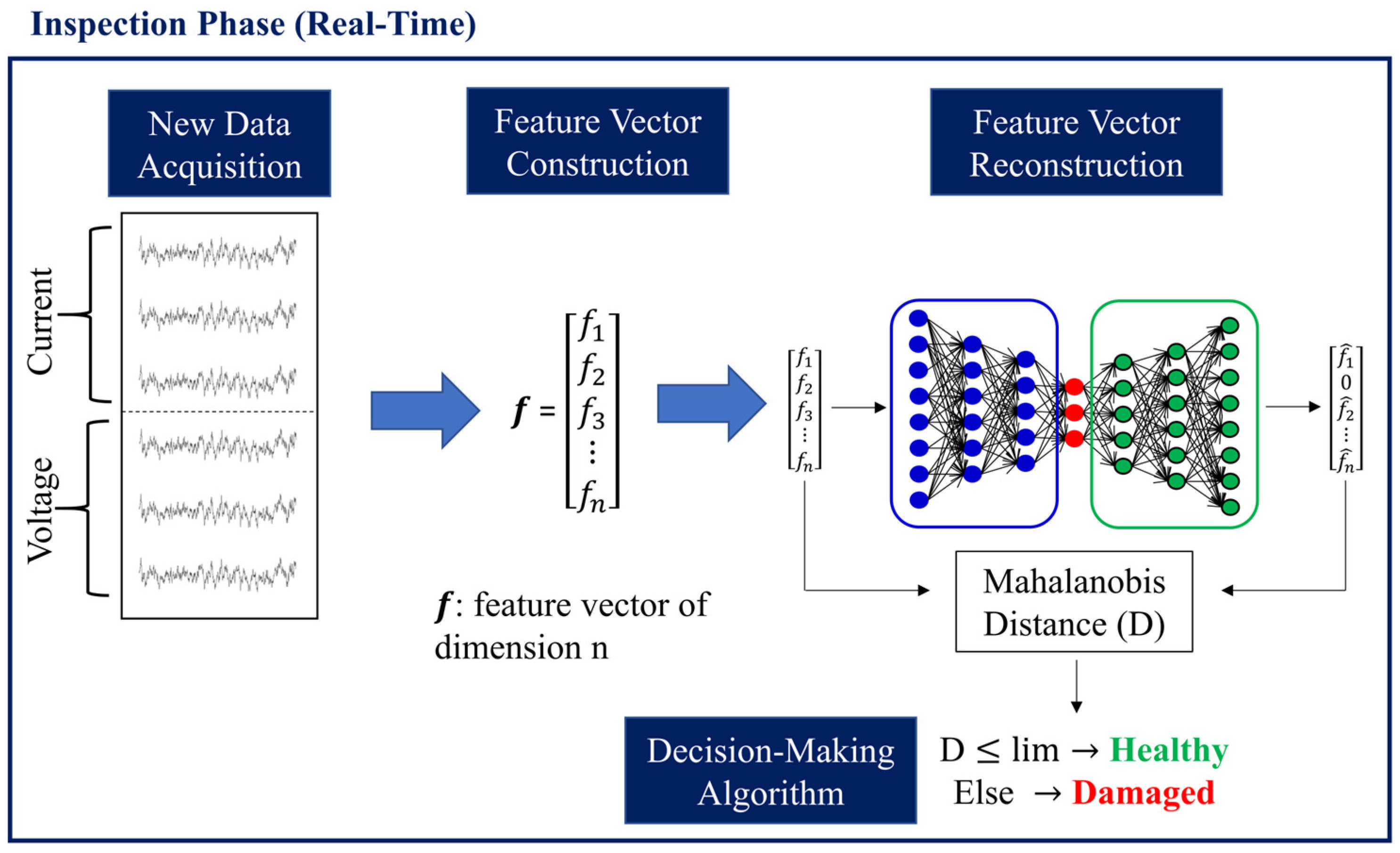
After completing the model configuration and training, the Inspection Phase commenced. It commenced by obtaining the new, unknown health condition time series with a sample length equivalent to the chosen window in TP Task 1. Subsequently, the feature vector was constructed using this acquired data. This feature vector was then inputted into the autoencoder, which aided in reconstructing the input feature vector. The next step involved calculating the statistical distance between the reconstructed and input feature vectors. The determination of the health status of the newly acquired data, as well as the system under monitoring, relied on a decision-making mechanism that was thoroughly explained in a relevant subsection. The Inspection Phase was further divided into the following five tasks:

IP Task 1: Data acquisition. Acquire fresh time series data for each of the n unique time series, ensuring a consistent sampling rate with the obtained training data, consisting of m samples.

IP Task 2: Feature construction. Construct the feature vector representing the current, unknown health state of the structure by combining the time series data acquired recently in the exact same sequence as during the TP.

IP Task 3: Compute the k-dimensional error vector. The autoencoder receives the new feature vector as input and reconstructs it in the output. Then, the k-dimensional error vector is calculated, excluding the values of the output that were nullified during the TP.

IP Task 4: Computation of the Mahalanobis distance. The Mahalanobis distance is calculated by utilizing the k-dimensional error vector, in addition to the sample mean value and sample covariance matrix obtained from TP Task 4.

IP Task 5: Decision of the structure’s integrity. The health condition or structural integrity is assessed by comparing the computed Mahalanobis distance from IP Task 4 to the user-defined threshold set during TP Task 5. If the Mahalanobis distance is less than or equal to the threshold, the unknown condition time series are categorized as healthy, indicating the overall health of the structure. Conversely, if the time series are classified as damaged, then the structure is also classified as damaged.

The IP tasks are depicted in Figure 3, where f represents the feature vector and f hat represents the reconstructed feature vector.

4.1. Autoencoder Backgorund Information

The autoencoder, an autoassociative artificial neural network, was utilized in this study to reconstruct input data. It is widely recognized for its ability to compress the input into a lower-dimensional latent space and then use this space to reconstruct the input data.

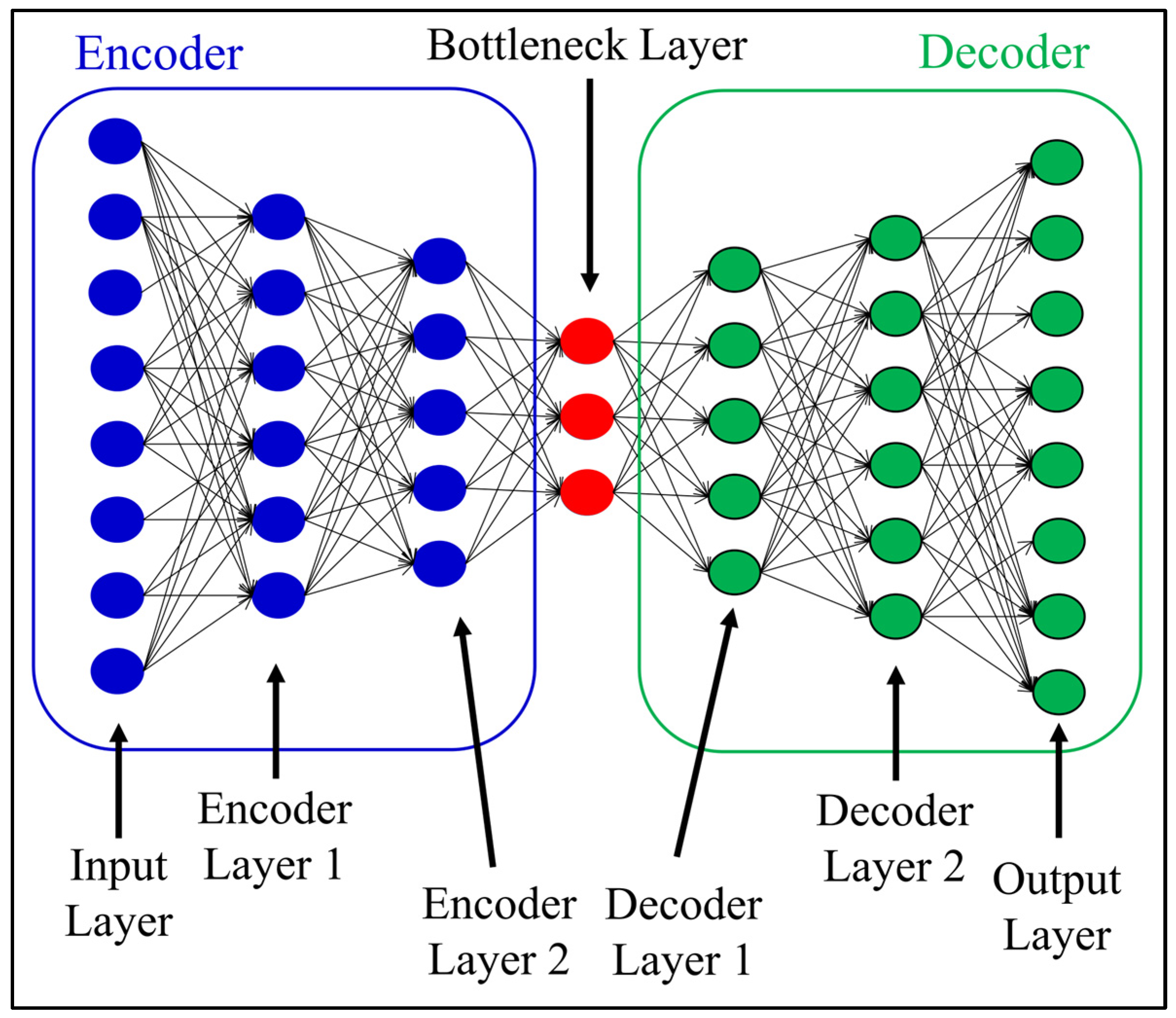
The autoencoder consists of two elements: the encoder and the decoder. The encoder includes input and encoder layers, while the decoder includes output and decoder layers. Both components have the same number of layers and neurons, as shown in Figure 4, ensuring the decoder mirrors the encoder. The intermediary layer, called the bottleneck layer, compresses and transforms the feature vector into a latent space. This latent space preserves important information for reconstructing the original feature vector.

The key concepts of a neural network and, subsequently, the autoencoder’s, are the activation function and the loss function. The activation function of a layer is a function that is applied to each neuron of the layer and transforms the output according to the activation function. Usually, the activation function is selected to be nonlinear in order for the autoencoder to learn more complex relationships.

The training of the autoencoder was a mathematical optimization problem. The function to be optimized was named the loss function. The loss function counted the difference between the actual output and the target output defined by the user. The target output in an autoencoder was the input itself. Different loss functions to be minimized were available such as mean absolute error, mean squared error, etc. The loss function selected was case-specific, but the general rule was that the lower the loss function, the better the training.

4.2. Autoencoder Configuration

In the present study, the autoencoder configuration consisted of an encoder with three layers: the input layer, the dense encoder layer 1 with 54 neurons, and an additional dense encoder layer 2 with 30 neurons. The bottleneck was represented by a dense layer with 20 neurons. The reduced feature vector obtained from the bottleneck was then passed to the decoder, which comprised a dense decoder layer 1 with 30 neurons, an additional decoder layer 2 with 54 neurons, and ended with the dense output layer consisting of 72 neurons, mirroring the encoder architecture. The selection of the number of neurons and activation functions was performed via a grid search. It is important to note that the grid search revealed numerous combinations that can achieve satisfactory results in damage detection, thus demonstrating the robustness of the methodology. The number of neurons in the bottleneck layer was crucial and should be equal to or greater than the number of variabilities in the system [12].

The activation functions used in the different layers primarily consisted of rectified linear unit (ReLU), except for the bottleneck layer, which incorporated a sigmoid activation function. The autoencoder’s training process involved the utilization of the Adam optimization algorithm [17], which is an extended version of stochastic gradient descent, along with the mean absolute error (MAE or L1) loss function. To prevent overfitting, an early stopping mechanism was implemented with a patience parameter set at 5. This meant that if the validation loss did not decrease after 5 consecutive epochs, the training process was terminated. For more comprehensive information about the autoencoder model, please refer to

Table 1. Details of the implemented autoencoder model.

Layer	Dimensionality	Activation Function
Input	72	-
Encoder 1	54	ReLU
Encoder 2	30	ReLU
Bottleneck	20	Sigmoid
Decoder 1	30	ReLU
Decoder 2	54	ReLU
Output	72	ReLU

Total parameters: 12 476; epochs: 1 000; batch size: 100; validation split: 10%; optimization algorithm: Adam; function loss: mean absolute error (MAE or L1).

.

4.3. Mahalanobis Distance Background Information

There are many statistical distance metrics available for measuring the difference between the original feature vector and its corresponding autoencoder reconstructed form. However, these metrics often overlook the impact of environmental and operating conditions commonly found in infrastructure settings, which can introduce significant variability. To address this concern, the Mahalanobis distance (D) was a suitable statistical distance metric. It incorporated the sample covariance and sample mean vectors, resulting in a more contextually relevant evaluation of the dissimilarity between the initial and reconstructed feature vectors. The Mahalanobis distance quantified the distance between a point and a multivariate distribution.

$$\mathrm{D}=\sqrt{{\left(x-\mu \right)}^T{\left[\mathsf{\Sigma }\right]}^{-1}\left(x-\mu \right)},$$

(1)

where x is the multidimensional vector of the point and μ the mean vector and Σ the semi-positive covariance matrix of the multivariate distribution.

4.4. Mahalanobis Distance Use

In this study, the Mahalanobis distance served as a measure of the distance between a feature vector and a set of feature vectors that formed a multivariate distribution. The error vector, denoted as x, represents the difference between the reconstructed feature vector and the actual feature vector. It is important to note that the length of x was inherently shorter than the initial feature vector. The sample mean value (μ) and sample covariance matrix (Σ) were computed using the k-dimensional error vectors from the training set. This indicated that the framework for damage detection remained unsupervised.

4.5. Decision-Making Mechanism

The determination of damage detection relies on evaluating the Mahalanobis distance (D) against a threshold value (lim). If the calculated distance is equal to or lower than the specified threshold, it implies that the feature vector represents healthy signals and, consequently, a healthy structure. Conversely, if the distance exceeds the threshold, it signifies the presence of damage in the signal, indicating structural damage in the monitored system. This uncomplicated decision-making process outlined in Equation (2) establishes a distinct boundary for determining the structural health status using the Mahalanobis distance metric.

$$\begin{gathered} \mathrm{D}\le lim\to \mathrm{Healthy} \\ \mathrm{D}>lim\to \mathrm{Damaged} \end{gathered}$$

(2)

5. The Experimental Test Case

The data presented in this document was meticulously obtained and gathered from a small, antiquated hydroelectric power plant (over 35 years old). This small hydropower plant comprises three Kaplan turbines and is able to create 10 MW of electricity. These generators were specifically designed to provide electricity to the general public as well as for self-consumption purposes. To ensure accurate data collection, a programmed system was implemented to collect data at consistent five-minute intervals. Subsequently, this data was transferred to the cloud for further analysis and evaluation.

5.1. Data Quality

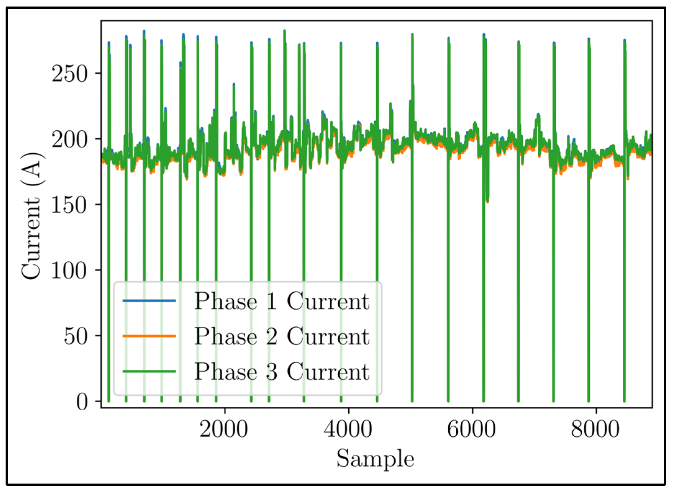
The extensive database contained a total of 94 unique types of measurements. These measurements covered important physical quantities such as current, voltage, power, and other relevant attributes. They were not only recorded for each individual phase but also for the line-to-line values of the star configuration of three-phase electric power. The dataset represented a continuous flow of measurements starting from 20 July 2023, until the end of the observational period on 20 August 2023. Throughout this time frame, a total of 8901 recorded samples per physical quantity were documented as time series. Figure 5 visually represents the current time series.

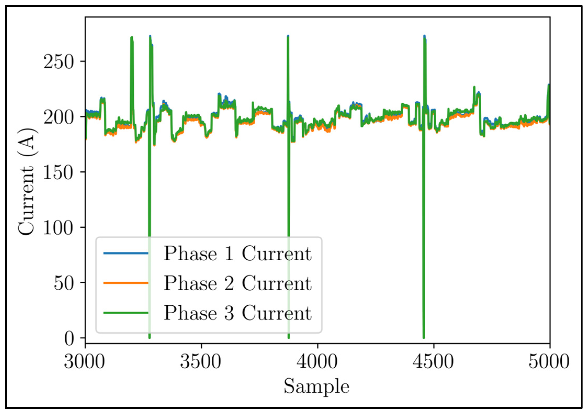
Figure 6 displays a magnified version of Figure 5. This enlarged image highlights the distinct variations in the time series of phase currents, indicating an uneven distribution of voltage load within each phase. Upon closer examination of the signals, it becomes evident that there was a recurring pattern, suggesting the presence of seasonality. These periodic fluctuations in current demand exhibited discernible peaks and valleys, occurring throughout the day.

A systematic analysis of relevant statistical metrics was carried out to evaluate the stationarity of these signals. The results of this investigation revealed that the signals were nonstationary, suggesting the existence of evolving dynamics over time and uncovering the intricate nature of the system.

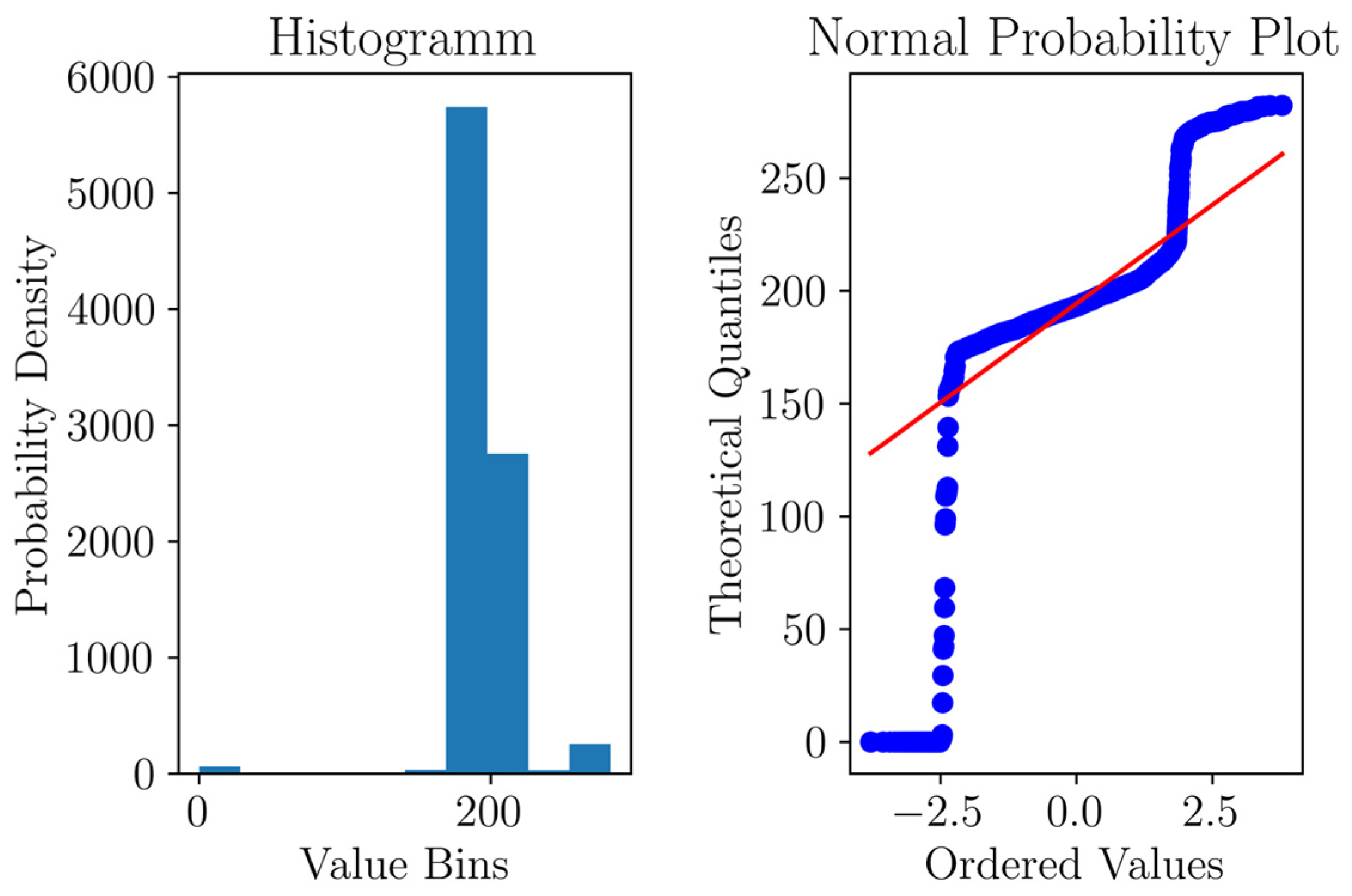
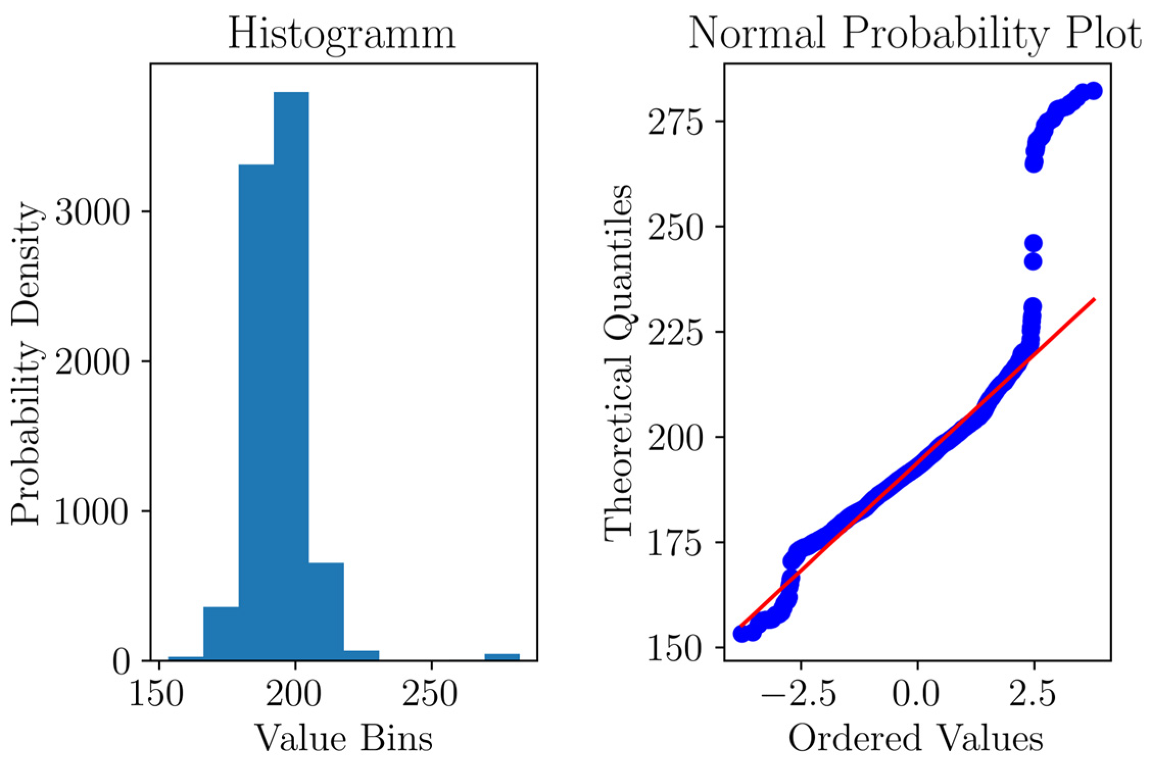
Figure 7 provides a detailed examination of the normal probability plot and histograms. It was evident that the data exhibits a Gaussian-like behavior, with a concentration of data points in the central region. However, there were a significant number of values that extended into the tails of the distribution. One notable feature of the dataset was the presence of a distinct pattern. This pattern indicated instances when the hydroelectric plant came to a halt or was intentionally deactivated, as the current values reached zero. Upon reactivation, the current values temporarily exceeded the ‘normal’ values, revealing an overshoot pattern.

5.2. Data Preprocessing and Splitting

Data preprocessing is a crucial step in obtaining valuable insights from data. It involves carefully cleaning, correcting, and manipulation of the data to ensure accuracy and reliability. In the context of predictive maintenance, this process plays a vital role in achieving high levels of proficiency.

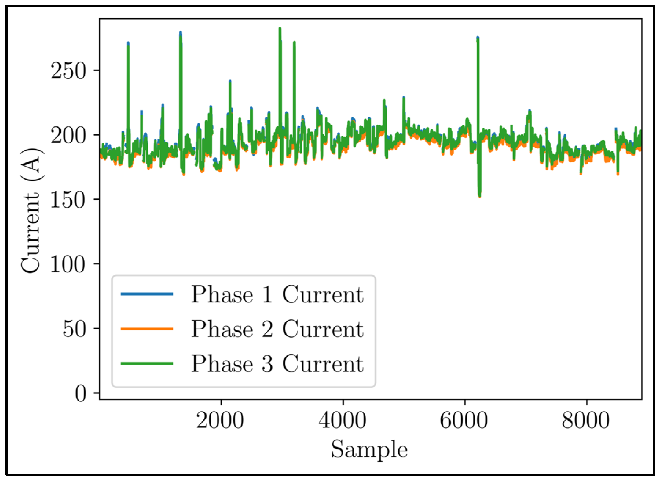
To address the issue of overshooting phenomena during power plant reactivation, a simple filtering approach was employed. This approach identified instances where the current phase value was zero, indicating power plant deactivation. The five data points preceding and the twenty-five data points following these zero values were then removed. The remaining parts of the time series were then joined together.

Figure 8 depicts the curated time series of phase currents, which was refined by eliminating the overshooting phenomena. The removal of these values resulted in a dataset consisting of 8276 samples. Furthermore, the dataset, which represented the indicative phase currents shown in Figure 8, then exhibited a normal distribution, as illustrated in Figure 9. In order to preserve the inherent characteristics of the dataset and account for the seasonality of the data, conventional normalization techniques such as division by standard deviation or mean correction were disregarded. This strategic decision ensured that the dataset remained intact.

Within the extensive dataset, only the effective phase currents and effective phase voltages were carefully chosen as sensitive features that could potentially indicate damage. This thorough selection process yielded a total of six physical quantities (three effective phase currents and three effective phase voltages). This decision was made based on the understanding that the remaining physical quantities in the dataset were deterministic byproducts of the phase currents and voltages. As a result, these additional physical quantities did not offer substantial insights into the structural health status, thus justifying their exclusion from the analysis. Additionally, according to [6], the current and voltage are directly affected by the irregularities that corrosion introduces and therefore an analysis on additional measurements/physical quantities was not required.

In the present study, the framework was evaluated in the aforementioned scenario, where the automated damage detection protocol can function in two ways. Firstly, it can operate on an hourly basis, taking advantage of the availability of 12 fresh samples. Alternatively, it can function every 5 min, incorporating the new measurement as the 12th sample for feature construction. This involved utilizing the previous 11 samples along with the newly acquired sample from the system. In both cases, the feature vector was constructed by combining 12 samples from each distinct measurement type.

The dataset available for analysis consisted of six different types of measurements, including three effective phase currents and three effective phase voltages. Each measurement type had a total of 8276 samples. These samples were collected over a period of less than one month, with a sampling period of 5 min. The dataset was preprocessed to remove any overshoot samples. To facilitate the analysis, the dataset was divided into training and testing sets. Each set contained 50% of the overall data, which corresponded to 4138 samples per set. To extract features from the dataset, the approach described in TP Task 1 was implemented.

A total of 344 72-dimensional feature vectors were generated by considering 12 samples (12 samples × 6 measurement types). Out of these 344 feature vectors, 34 (10%) were set aside for model validation, while the remaining 310 (90%) were used for training purposes. The testing set was divided into two distinct subsets, namely testing subset 1 and testing subset 2. Each subset consisted of 172 feature vectors, which accounted for 50% of the initial testing set. This division of the test set was implemented to differentiate between the healthy inspection cases and the ones used to simulate damage scenarios.

5.3. Damage Scenarios

A prevalent issue that frequently occurs in aging power plants is the corrosion of conductors in generators, which can have detrimental effects on their performance. This corrosion can lead to changes in impedance, signal reflections, and other irregularities, resulting in the introduction of noise into the measured sinusoidal signal. Consequently, this compromises the power production of the plants. This particular type of damage significantly reduces power production and overall efficiency in environmentally friendly power plants. Therefore, the timely and prompt detection of such damage scenarios is of utmost importance, as it has the potential to mitigate the negative impacts on power generation and efficiency.

In order to replicate conductor corrosion, synthetic white Gaussian noise was introduced into the measurement of a single-phase current. This noise was generated from a normal distribution with a mean of zero and different standard deviations, which were approximately 5%, 10%, and 20% of the standard deviation of the entire preprocessed current signals. As a result, three discrete damage levels were created, referred to as DS1, DS2, and DS3, as shown in

Table 2. Details of the implemented damage scenarios, training, and validation sets.

Dataset Name	Damage Level (Standard Deviation of W.N.)	No. of Feature Vectors
Training	-	310
Validation	-	34
Testing Subset 1	-	172
Testing Subset 2	-	172
Damage Scenario 1 (DS1)	‘Low’ std = 0.5 (~5%)	172
Damage Scenario 2 (DS2)	‘Medium’ std = 1 (~10%)	172
Damage Scenario 3 (DS3)	‘High’ std = 2 (~20%)	172

The noise sets were created from Testing Subset 2 via the addition of noise to the first 12 features of the feature vector. The 12 first features corresponded to first single-phase current.

. The noise was generated using a random sampling routine from the NumPy library in Python and was then added to each feature vector within testing subset 2. This process produced three polluted sets, namely sets 1, 2, and 3, each characterized by a distinct level of noise. To ensure reproducibility, unique seed numbers were used for each simulated noise, and the noise was only incorporated into the first 12 samples of the feature vector corresponding to the first single-phase current. This added an additional layer of difficulty in detecting the noise.

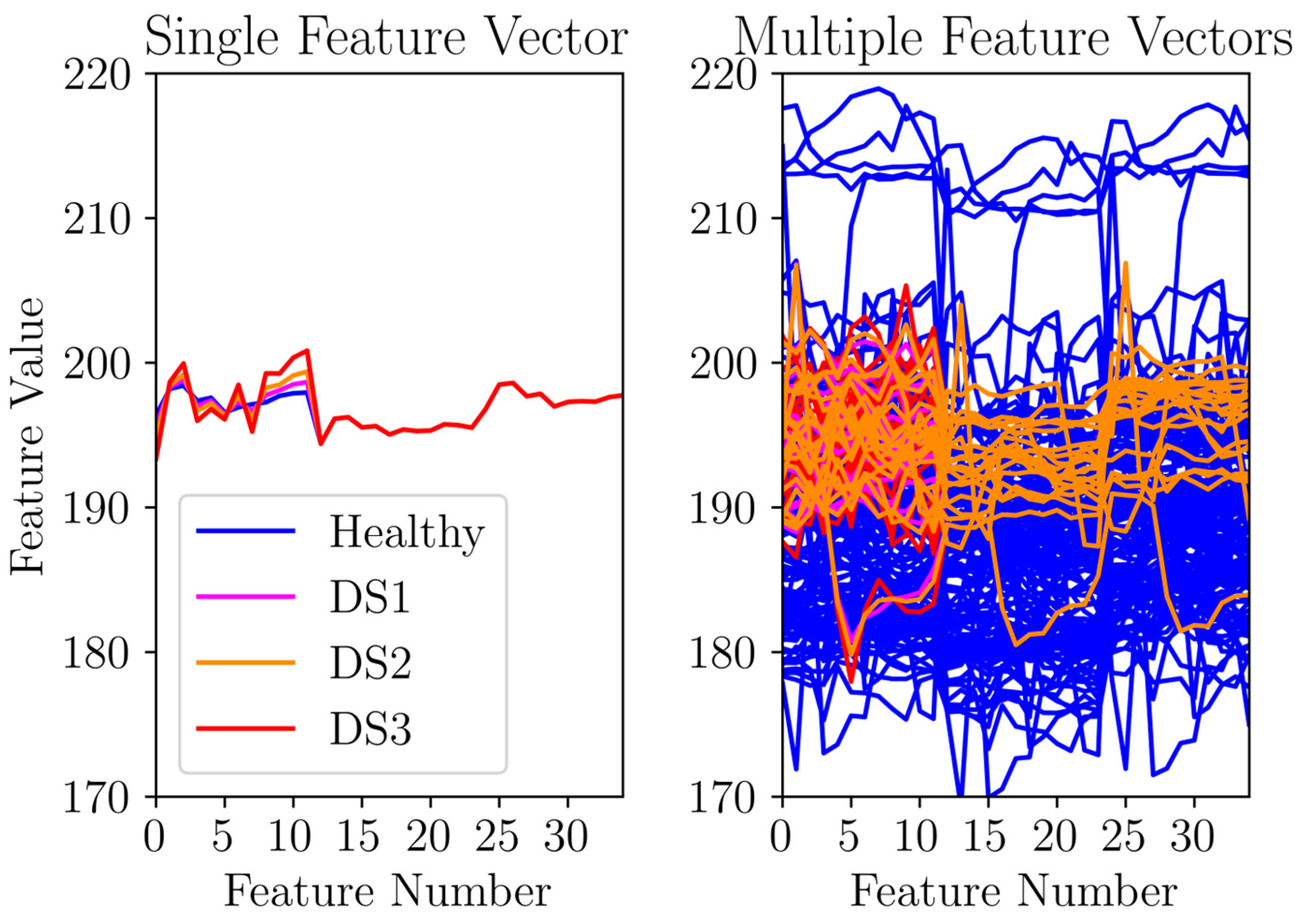
In Figure 10, the left subplot demonstrates that the noise levels introduced were quite subtle, making it difficult to perceive them visually. Additionally, the right subplot in Figure 10 further supports this observation by showing that the incremental noise addition was hardly noticeable when compared to the ‘healthy’ feature vectors. This almost imperceptible nature of the added noise highlighted the challenge of detecting subtle variations and emphasized the necessity of a strong and sensitive damage detection framework to accurately differentiate these subtle changes caused by ‘damage’ from the healthy signals amidst variability.

5.4. Training of the Autoencoder Model

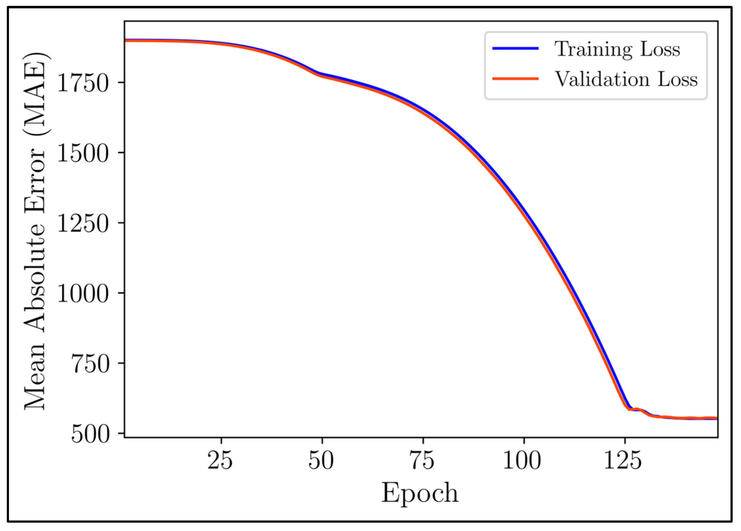
The dataset for training consisted of 344 feature vectors. In order to facilitate the training of the model, 90% of this dataset, which was equivalent to 310 vectors, was utilized for training. The remaining 34 vectors were set aside as a validation set. Figure 11 visually displays the training and validation loss curves of the autoencoder model.

The trend that has been observed indicated a consistent decrease in the training loss until it reached a point of stagnation, which typically occurred around the 148th epoch. This pattern was also reflected in the validation loss, suggesting that the model effectively fitted the training data without succumbing to overfitting. However, despite the seemingly adequate fitting, the overall loss remained relatively high. This can be attributed to instances where the model outputted zeros, leading to a significant dissimilarity between the reconstructed and initial feature vectors. To address this issue, the damage detection procedure only considered nonzero values, thereby reducing the impact of zeroed outputs on the assessment. It is important to note that the utilization of the ReLU activation function was responsible for the emergence of these zero values, underscoring the importance of selecting the most critical feature elements. Furthermore, during the damage detection phase, the complete feature vector was inputted into the autoencoder model, but only the nonzero values were used to compute the error vector and subsequently the Mahalanobis distance.

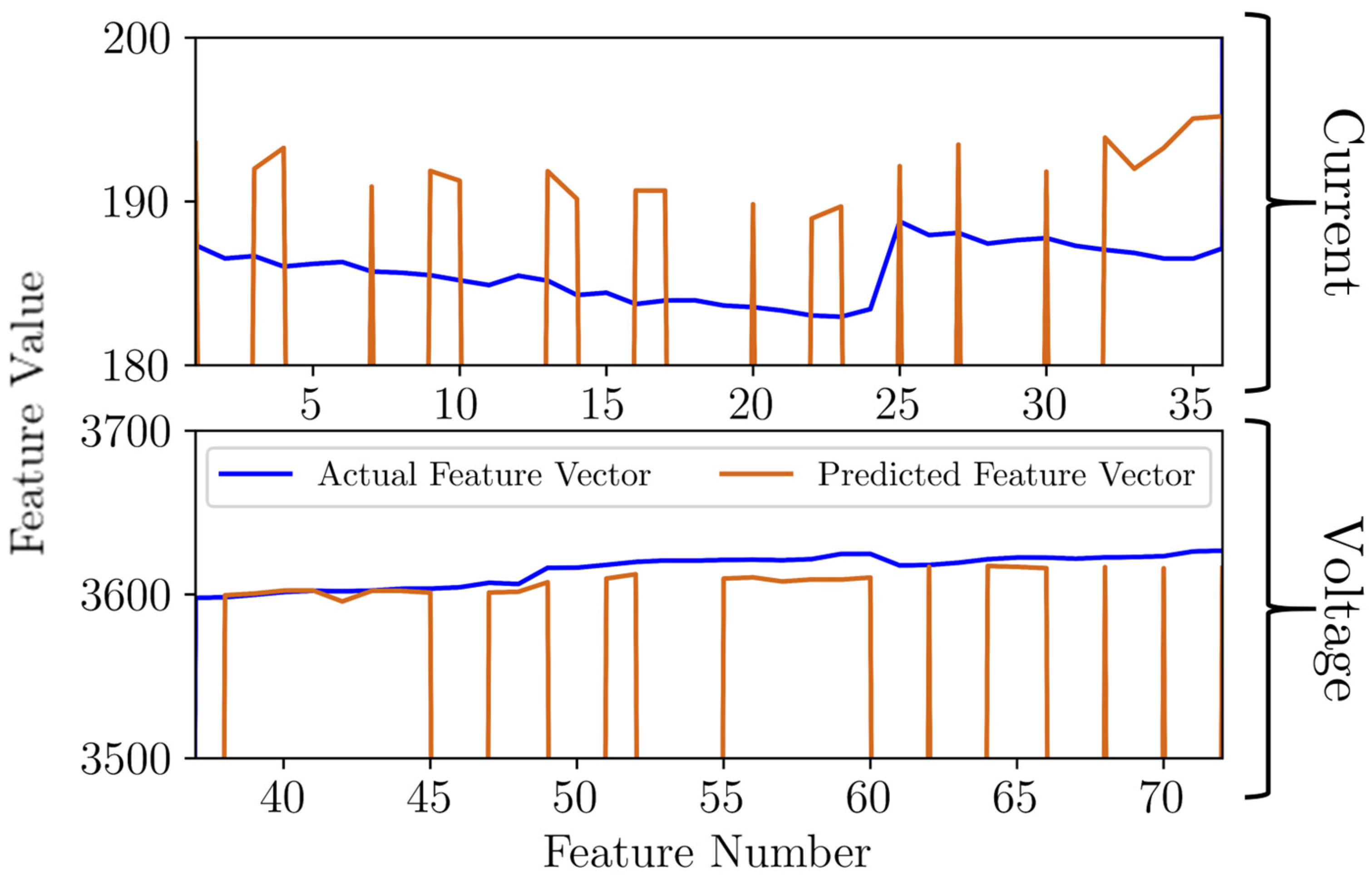
Figure 12 presents a representative reconstruction of a healthy feature vector. It is worth noting that the reconstructed feature vector displayed variations in comparison to the actual values. Nevertheless, the overall reconstruction was considered satisfactory. An important aspect mentioned earlier is clearly visible in this figure, which is the presence of zero values. Despite these zero values, the reconstruction effectively captured essential features, highlighting the model’s ability to delineate critical information even in the presence of these null elements. It is important to mention that the percentage errors of current and voltage were identical. However, due to the higher voltage values, the absolute errors of voltage appeared to be lower, resulting in a seemingly more accurate prediction.

6. Damage Detection Results

To evaluate a framework accurately, it was crucial to choose unbiased statistical assessment tools that can facilitate a comparison of the results with a benchmark framework. Once the tools were selected, the method was assessed, and the detailed results of the assessment tools were presented. This study followed a two-step process, where the assessment tools were presented first, followed by the results. It was important to highlight that no specific threshold, as described in the Training Phase, was chosen. The assessment tools evaluated all potential thresholds, thereby assessing the framework with all possible combinations.

6.1. Assesment Tools

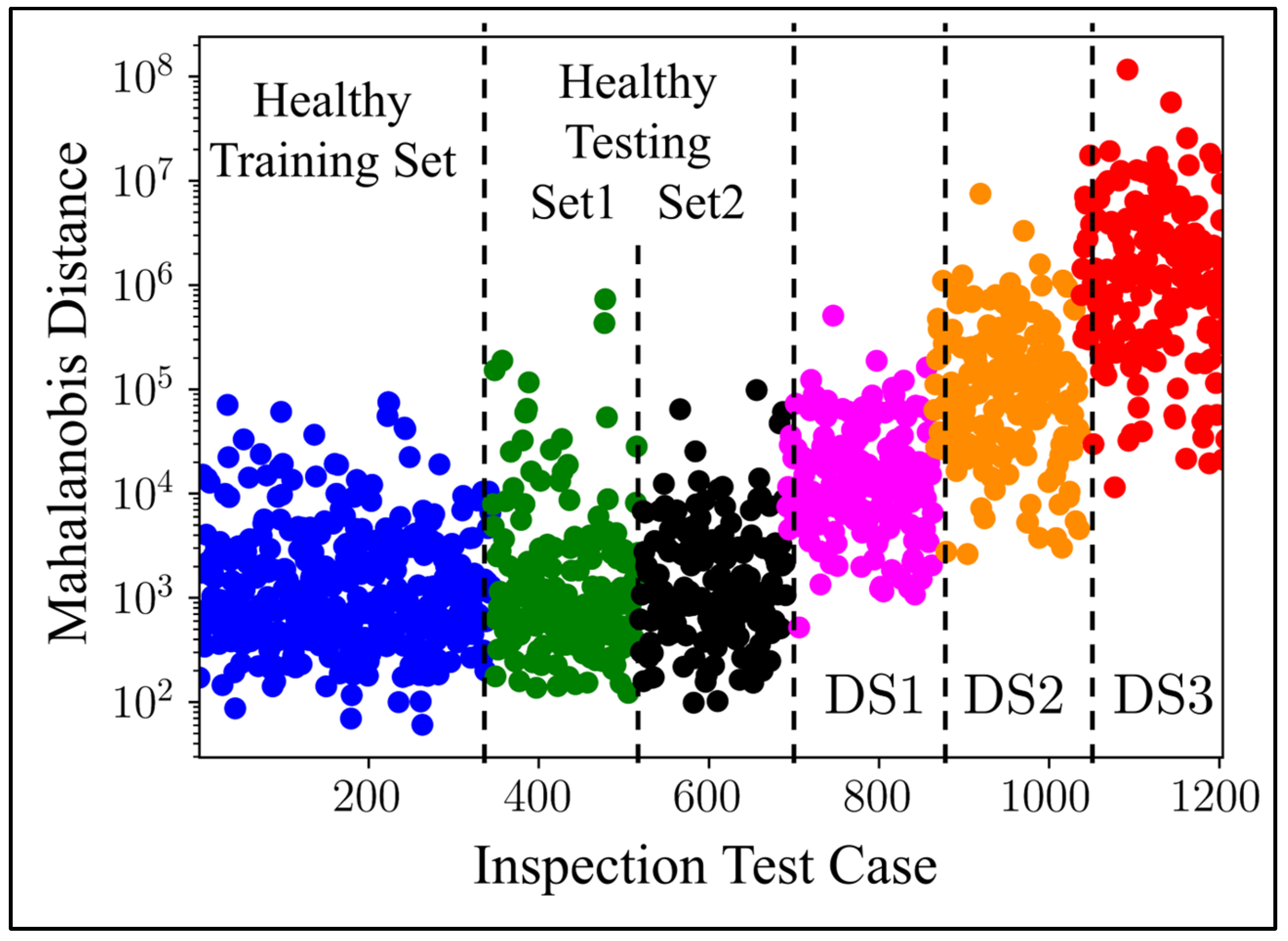
The proposed damage detection framework was evaluated using scatter plots and receiver operating characteristic (ROC) curves [24]. Scatter plots are proven to be an effective assessment tool as they allow for the visualization of results by comparing the distances calculated for the damaged signals with those of the healthy signals. This visual representation provides a clear understanding of the detectability of the damage. If the distances for the damaged signals are higher than those of the healthy signals, it indicates that the damage can be easily detected using the employed algorithm. On the other hand, if the distances for the damaged signals align with or are lower than those of the healthy signals, it becomes challenging to distinguish the damage from the healthy signals.

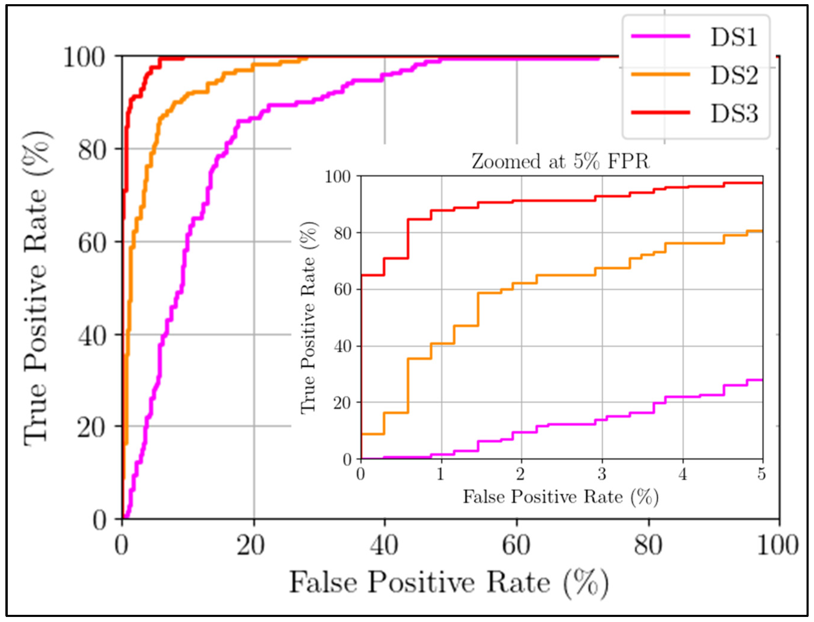
The ROC curve is a statistical tool that plots the false positive rate (FPR), which represents false alarms, against the true positive rate (TPR), which indicates correct damage detection. An ideal performance is achieved when a 0% FPR corresponds to a 100% TPR, indicating perfect classification. The advantage of the ROC curve is its insensitivity to the imbalanced number of positive and negative test cases. Typically, a specific FPR is chosen to facilitate the comparison of TPR, allowing for the evaluation of the classifier’s effectiveness in different damage scenarios.

6.2. Results

The scatter plot in Figure 13 visually illustrates the damage detection outcomes of the autoencoder. It was evident that the autoencoder struggled to differentiate between the healthy datasets and the damage scenario DS1. However, DS2 and DS3, which represent moderate and high levels of damage, respectively, show distinct differences and were easily detected by the autoencoder. This observation highlighted the robust performance of the proposed damage detection framework in identifying moderate to severe noise levels, emphasizing its effectiveness in the current study.

Figure 14 displays the ROC curves for each damage scenario. It is worth noting that DS2 and DS3 achieved true positive rates (TPR) exceeding 80% at a false positive rate (FPR) of 5%, indicating a strong ability to detect ‘medium’ and ‘high’ level damage, which aligned with the scatter plot findings. On the other hand, the ‘low’ level damage scenario (DS1) posed a significant challenge, exhibiting a lower TPR at the same 5% FPR threshold, suggesting a relatively lower detectability for this specific severity of damage.

To summarize, the proposed damage detection framework in this study exhibited impressive performance, particularly in identifying damage of ‘medium’ to ‘high’ severity levels. In comparison to existing commercial physics-based methods, this approach not only detects but also visualizes the progression of damage through scatter plots. The combination of these results’ easy interpretability makes them highly appealing for further research and future industrial implementation.

6.3. Comparative Analysis

To facilitate a comparative analysis of the proposed model with a well-known machine learning algorithm, the support vector machine classifier was used. The hyperparameters utilized adhered to the default values of the Python library used by [25], specifying a radial basis function (RBF) kernel with regularization parameter C set to 1 and gamma set as ‘scaled’. The classifier underwent training utilizing the same healthy training and validation dataset as the autoencoder, along with the inclusion of 86 feature vectors per damage scenario (50%), amounting to 258 in total. Within this dataset of 86 feature vectors, nine (10%) were used as a validation subset (27 as a validation subset and 231 as a training subset). Consequently, the accuracy of the classifier was assessed based on a dataset comprising 344 healthy feature vectors (healthy test subsets 1 and 2) and the remainder of 258 (50%) damaged feature vectors. The resultant accuracy achieved by the classifier was recorded at 81.5%. It is noteworthy that a grid search for optimizing the classifier’s hyperparameters was not performed in this analysis. Consequently, it is acknowledged that the absence of this optimization process may slightly reduce the performance of the method.

In assessing the accuracy of the autoencoder, an optimal threshold was employed. Each data point on the ROC curve corresponded to a specific threshold value. By definition, the optimal threshold was determined as the point on the ROC curve that minimized the distance from said point to the ideal detection point (0,1). This threshold was 4772 and was computed from an aggregative ROC curve that did not differentiate the damage scenarios as presented in Figure 14. The achieved accuracy was 87.3% and is presented in

Table 3. Comparative analysis results.

Method	Accuracy
Autoencoder coupled with Mahalanobis distance	87.3%
SVM classifier	81.5%

.

It is important to highlight that for a meaningful comparison, the accuracy computation of the autoencoders was performed using the identical sets of feature vectors utilized in the SVM classifier. Notably, the autoencoder, when coupled with the Mahalanobis distance metric, exhibited slightly better performance compared to the SVM classifier. Additionally, the unsupervised nature of the autoencoder gave it an edge over its counterpart. The accuracy results of both methods are presented in Table 3.

7. Discussion

The implementation of a corrosion detection framework in an operational power plant is an extremely demanding process. The existing data acquisition system has already been monitored in an aged hydropower plant and has demonstrated its feasibility. However, retrofitting a system into an aged infrastructure poses compatibility challenges. Once the data acquisition system is installed, ensuring data quality becomes crucial, as noisy or inaccurate data can result in biased or undesired models. Given the presence of changing environmental conditions, it is essential for the data to capture environmental variability in order to develop a robust model that can handle EOCs effectively. Furthermore, the deployment and maintenance of sensors play a critical role in the effectiveness of corrosion detection, as any issues may lead to false alarms. In terms of real-time detection, once the system is trained, it does not require excessive resources, thus avoiding power consumption concerns. However, integrating the framework/system with existing monitoring and control systems in hydropower plants can be challenging. Compatibility issues may arise, and seamless integration is vital for practical implementation. The cost associated with deploying and maintaining the corrosion detection framework should also be taken into consideration, as cost-effectiveness is a crucial factor in determining the feasibility of the solution. Additionally, it is important to note that over time, the performance of the model may degrade due to changes in the environment or system dynamics. Therefore, regular updates and retraining may be necessary to ensure long-term effectiveness.

Once the obstacles have been overcome and the system is operational, it will have the capability to optimize power production in the power plant by promptly detecting corrosion and assisting the MRO crew in replacing the conductors. By enhancing the current and voltage quality, efficient energy production will be achieved, resulting in an overall increase in energy production from renewable sources. This will contribute to meeting the European quotas for 2030 and pave the way for a more sustainable energy sector. The proposed framework itself is scalable, but the main concern lies in the scalability of the data acquisition system. The acquisition system needs to be able to scale with the geometric dimensions of the conductors it monitors, as well as the values and accuracy it can record. The framework is both robust and scalable, with the scalability aspect primarily focused on the hardware it utilizes. Therefore, the framework can be used in additional industries that use generators and are susceptible to corrosion.

8. Conclusions

Hydropower plants are a valuable and efficient source of low-carbon electricity, according to the International Energy Agency (IEA). The data for 2020–2030 shows that hydropower plants are preferred in developing and emerging economies over other renewable alternatives and fossil fuels [26]. These nations have untapped potential for hydropower, which can meet the growing demand for flexible electricity. However, the aging components of hydropower plants can lead to extensive, costly, and risky maintenance, causing significant environmental, societal, and economic consequences.

A robust framework integrating an autoencoder with the Mahalanobis distance technique has been introduced to tackle this challenge. This framework can identify damage of different severity levels, considering the impact of environmental and operating conditions. The framework was evaluated through one hundred test experiments in a real-world scenario. Data from a hydropower plant was collected using a hybrid data fusion approach and securely transmitted wirelessly for analysis. The key innovations of this study were the use of unsupervised AI-based techniques for corrosion detection and the analysis of real-world data.

The study’s primary findings regarding the development and evaluation of the framework revealed that the unsupervised framework effectively detected artificial damage (noise) and achieved diagnostic scores with a true positive rate (TPR) surpassing 80% at a false positive rate (FPR) of 5%. This framework demonstrated its efficacy in identifying damage of ‘medium’ to ‘high’ severity levels. It is worth noting that this level of performance was attained using only 50% of the available training data, highlighting its resilience. Corrosion is an ongoing and progressive process, and its effects may not be immediately evident in current measurements. Therefore, the authors have taken a proactive approach by introducing simulated damage for immediate evaluation. This simulated damage, created by introducing noise, aimed to replicate the impact of corrosion on a single-phase conductor and imitate its outcomes. The accuracy of the corrosion detection results was closely tied to the ability of the artificial damage to mimic the actual damage, which partially restricted the assessment procedure.

Moving forward, the focus will be on creating a system that assists and guides the MRO crew, implementing it in a power plant, addressing the issues highlighted in the discussion section, and analyzing the feasibility and economic viability of this support system. The primary concern is whether the real-time detection of corrosion and maintenance of conductors will enhance energy production enough to offset the costs of the system.