Multivariate Time-Series Forecasting: A Review of Deep Learning Methods in Internet of Things Applications to Smart Cities

Abstract

Smart cities are urban areas that utilize digital solutions to enhance the efficiency of conventional networks and services for sustainable growth, optimized resource management, and the well-being of its residents. Today, with the increase in urban populations worldwide, their importance is greater than ever before and, as a result, they are being rapidly developed to meet the varying needs of their inhabitants. The Internet of Things (IoT) lies at the heart of such efforts, as it allows for large amounts of data to be collected and subsequently used in intelligent ways that contribute to smart city goals. Time-series forecasting using deep learning has been a major research focus due to its significance in many real-world applications in key sectors, such as medicine, climate, retail, finance, and more. This review focuses on describing the most prominent deep learning time-series forecasting methods and their application to six smart city domains, and more specifically, on problems of a multivariate nature, where more than one IoT time series is involved.

1. Introduction

A smart city is a place where traditional networks and services are improved by utilizing and embracing contemporary technological principles for the benefit of its citizens [1]. Smart cities are being rapidly implemented to accommodate the continuously expanding population in urban cities and provide them with increased living standards [2]. Going beyond the use of digital technologies for better resource use and less emissions, the development of smart cities entails smarter urban transportation networks, more responsive and interactive administration, improved water supply and waste disposal facilities, more efficient building lighting and heating systems, safer public places, and more. To this end, smart cities employ Internet of Things (IoT) devices, such as connected sensors, embedded systems, and smart meters, to collect various measurements at regular intervals (time-series data), which are subsequently analyzed and ultimately used to improve infrastructure and services [3].

Deep learning algorithms [4], renowned for their ability to extract intricate patterns from complex datasets, have proven particularly adept at handling the multifaceted time-series data characteristic of smart city IoT applications. These algorithms are designed to capture the dynamics of multiple time series concurrently and harness interdependencies among these series, resulting in more robust predictions [5]. Consequently, deep learning techniques have found application in various time-series forecasting scenarios across diverse domains, such as retail [6], healthcare [7], biology [8], medicine [9], aviation [10], energy [11], climate [12], automotive industry [13] and finance [14].

Remarkable examples of these technologies in action include Singapore’s Smart Nation Program around traffic-flow forecasting, Beijing’s Environmental Protection Bureau ‘Green Horizon’, the City of Los Angeles’ ‘Predicting What We Breathe’ air-quality forecasting projects, and the United States Department of Energy SunShot initiative around renewable energy forecasting. More specifically, in Singapore, the Land Transport Authority has created a traffic management system powered by AI that analyzes real-time data to optimize traffic flow and alleviate congestion. In Beijing, IBM’s China Research Lab has developed one of the world’s most advanced air-quality forecasting systems, while across multiple cities in the United States, IBM is making renewable energy-demand and supply forecasts.

Beyond their technical implications, the implementation of such technologies brings profound socioeconomic and environmental outcomes for cities and their residents [15]. Indicatively, it can foster economic growth by attracting talented individuals and entrepreneurs, potentially turning cities into innovation hubs, which, in turn, can lead to job creation and increased economic competitiveness [16]. As smart cities become more prosperous through economic growth, healthcare and education become more accessible and more inclusive, which results in more engaged and empowered citizens, contributing to social cohesion and overall well-being [17]. Moreover, AI-driven efficiency improvements in resource management can make cities more environmentally sustainable, addressing global challenges such as climate change [18].

There have been several surveys around deep learning for time-series forecasting, both in theoretical [5] and experimental [19] contexts. Looking at smart cities, deep learning has been used in various domains, but since this is still an emerging application area, only a few surveys have studied the current state-of-the-art models. Many of these, such as [20,21], describe deep learning as part of a broader view of machine learning approaches and examine a limited number of models. Other studies focusing on deep learning methods consider a wide set of data types, such as text and/or images [22,23,24,25], or address tasks beyond forecasting (e.g., classification), thus not providing a comprehensive overview on time-series forecasting in IoT-based smart city applications. More importantly, these studies do not include research works pertaining to contemporary deep learning architectures (see

Table 1. Comparison of relevant survey papers.

Article	Field	Data Types	Deep Learning Algorithms					Smart City Domain
			CNN	RNN	Attention	GNN	Hybrid
[20]	ML + DL	Time series, images		X				Environment, mobility, living
[21]	ML + DL	Time series, images						Environment
[22]	DL	Time series, images, text	X	X			X	Environment, mobility, buildings, living
[24]	DL	Time series, images, text	X	X			X	Environment, mobility, living
[25]	DL	Time series, images, text	X	X			X	Environment, mobility, living
Our paper	DL	Time series	X	X	X	X	X	Environment, mobility

). This study endeavors to address this gap by providing a more recent and concise overview of how deep learning methods enhance smart cities through the modeling and forecasting of multivariate time-series IoT data.

Smart city applications can be grouped into six major domains [17]: smart environment, smart mobility, smart buildings, smart governance, smart living, and smart economy and people. In this paper, we focus on two domains—smart environment and smart mobility—that have witnessed the extensive adoption of deep learning methods (see Table 1), analyzing six prominent applications: air-quality, water-quality, and energy-demand management from the smart environment domain, and car park occupancy, traffic-flow monitoring, and passenger flow from the smart mobility domain. We intentionally narrow our scope to provide an in-depth examination of these applications, emphasizing the trends and dynamics of deep learning models for time-series forecasting within the context of smart cities.

The remainder of this paper is structured as follows: Section 2 introduces existing advances in deep learning algorithms for multivariate time-series forecasting, encompassing recurrent neural networks (RNNs), convolutional neural networks (CNNs), the attention mechanism, graph neural networks (GNNs), and their combinations. Section 3 delves into the applications of these models in the smart environment and smart mobility domains, exploring their characteristics, popularity, and performance. Section 4 highlights the challenges and limitations present in the existing literature, each paving the way for a discussion on future directions. Finally, Section 5 concludes with a summary of our study and offers insights into emerging trends in state-of-the-art deep learning models, considering their applicability to the reviewed domains.

2. Deep Learning Architectures for Multivariate Time-Series Forecasting

Deep learning architectures model complex relationships through a series of nonlinear layers—the set of nodes of each intermediate layer capturing the corresponding feature representation of the input [26]. In a time-series context, these feature representations correspond to relevant temporal information up to that point in time, encoded into some latent variable at each step. In the final layer, the very last encoding is used to make a forecast. In this section, the most common types of deep learning building blocks for multivariate time-series forecasting are outlined.

2.1. Recurrent Neural Networks

Recurrent neural networks have a long and well-established history when it comes to time-series forecasting [27] that continues to date. The core building block of RNNs is the RNN cells that essentially act as an internal memory state. Their purpose is to maintain a condensed summary of past information deemed useful by the network for forecasting future values. At each time step, the network is presented with fresh observations, and cells are updated accordingly with new information. The standard structure of an RNN and its unfolded-in-time version are shown in Figure 1. In the case of multivariate time series, the inputs x and outputs t are multidimensional in each of the time steps.

Older versions of RNNs were notorious for failing to adequately capture long-term dependencies, a problem commonly known as ’exploding and vanishing gradients’ [29]. More specifically, the lack of restriction on their look-back window range meant that the RNNs cells were unable to contain all the relevant information from the beginning of the sequence [30]. The advent of long short-term memory networks (LSTMs) [31] and other closely related variants, such as the gated recurrent units (GRUs [32]), largely alleviated this problem, by allowing the gradients to flow more stably within the network. In Figure 2, the different cells used by the LSTMs and GRUs are displayed.

Another shortcoming of conventional RNNs was the inability to make use of future time steps. To overcome this limitation, a new type of architecture, bidirectional RNNs (BiRNNs), was proposed by Schuster and Paliwal [34]. The novelty of BiRNNs was that they could be trained in both time directions at the same time, using separate hidden layers for each direction: forward layers and backward layers. Later on, Graves and Schmidhuber [35] introduced the LSTM cell to the BiRNN architecture, creating an improved version: the bidirectional LSTM (BiLSTM). Using the same principles, the bidirectional paradigm can be extended to GRUs to create BiGRU networks. A very common and powerful end-to-end approach to sequence modeling that utilizes LSTMs, GRUs, or their bidirectional versions is the sequence-to-sequence (Seq2seq) or encoder-decoder framework [36]. This framework originally had a lot of success in natural language processing tasks, such as machine translation, but can also be used in time-series prediction [37]. Under this framework, a neural network (the encoder) is used to encode the input data in a fixed-size vector, while another neural network takes the produced fixed-size vector as its own input to produce the target time series. Any of the mentioned RNN variants can act as the encoder or the decoder. Such an architecture can produce an entire target sequence all at once. All these advances and improvements to RNNs have resulted in them being established as the driving force behind many modern state-of-the-art multivariate time-series forecasting architectures, which use them as their main building blocks [38,39,40,41,42].

When utilizing RNNs and their variants, careful attention should be given to their hyperparameter tuning [43], especially in the selection of the number of hidden units, hidden layers, the learning rate, and the batch size. The number of hidden units and layers should align with the data complexity, and the more complex the data, the higher the number of layers and neural networks as a general rule of thumb. Adaptive learning rate techniques are essential to address nonstationarity, while the right batch size can ensure a smoother learning process. Lastly, for such models to thrive, it is important that the length of the input sequences should match the time patterns in it, especially if long-term connections are to be captured.

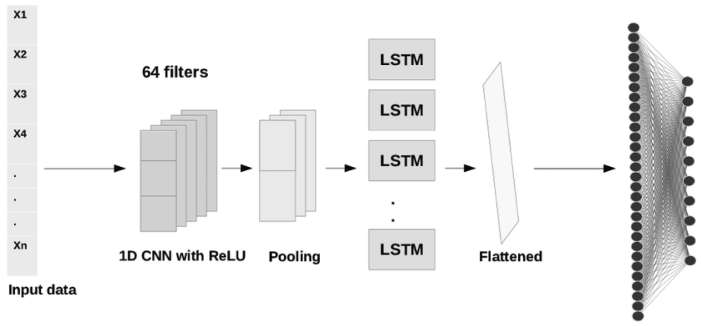
2.2. Convolutional Neural Networks

Convolutional neural networks were originally used for computer vision tasks. By making strong, but to a great degree correct, assumptions about the nature of images in terms of the stationarity of statistics and locality of pixel dependencies, CNNs are able to learn meaningful relationships and extract powerful representations [44].

CNNs typically consist of a series of convolutional layers followed by pooling layers, with one or more dense layers in the end. Convolutional layers perform a convolution operation of their input series with a filter matrix to construct high-level representations. The purpose of the pooling operation is to reduce the dimensionality of these representations while preserving as much information as possible. In addition, the produced representations are rotationally and positionally invariant. CNNs for time-series data, usually referred to as temporal CNNs and similar to standard/spatial CNNs, make invariance assumptions. In this case, however, such assumptions are about time instead of space, as they maintain the same set of filter weights across each time step. For CNNs to be transferred from the domain of computer vision to time-series forecasting, some modifications are needed [45,46]. A main concern is that the look-back window of CNNs is controlled by and limited by the size of its filter, also known as the receptive field. As a result, choosing the right filter size is crucial for the network’s capability to pick up all the relevant historical information, and finding an optimal size is not an easy task and is usually considered part of the hyperparameter tuning process [46]. Another consideration is related to the leakage of data from the future into the past; in [45], the so-called causal convolutions were developed to make sure that there is no leakage from the future into the past and only past information is used for forecasting. Lastly, to capture long-term temporal dependencies, a combination of very deep networks, augmented with residual layers, along with dilated convolutions, are employed, which are able to maintain very long effective history sizes [46]. An example of a CNN architecture for multivariate time-series forecasting can be seen in Figure 3. Since the number of parameters grows in line with the size of the look-back window, the use of standard convolutional layers can be computationally expensive, especially in cases where strong long-term dependencies are formed. To decrease the computational burden but maintain the desired results, newer architectures [45,47] often employ so-called dilated convolutional layers. Dilated convolutions can be viewed as convolutions of a downsampled version of the lower-level features, making it much less expensive to incorporate information from past time steps. The degree of downsampling is controlled by the dilation rate, applied on a layer basis. Dilated convolutions can, therefore, gradually accumulate information from various time blocks by increasing the dilation rate with each layer, allowing for more efficient utilization of historic information [5].

When it comes to hyperparameter tuning, focus should be directed towards the alignment of the number of filters, the filter sizes, the number of convolutional layers, and pooling strategies with the inherent patterns of the data [47]. More specifically, the more intricate and diverse the data are, the greater the number of filters and layers needed to capture it. Longer sequences contain more information and context and usually require larger filters to capture broader patterns and dependencies over extended periods. If the data are noisy, then pooling layers can help cut through the noise and improve the model’s focus on the features that matter.

2.3. Attention Mechanism

LSTMs acted to mitigate the problem of vanishing gradients, however, they did not eradicate it. While, in theory, the LSTM memory can hold and preserve information from the previous state, in practice, due to vanishing gradients, the information retained by these networks at the end of a long sequence is deprived of any precise, contextual, or extractable information about preceding states.

This problem was addressed by the attention mechanism [49,50], originally used in transformer architectures for machine translation [51,52,53]. Attention is a technique that helps neural networks focus on the more important parts of the input data and deprioritize the less important ones. Which parts are more relevant is learned by the network through the input data itself and is derived by the context. This is achieved by making all the previous states at any preceding point along the sequence available to the network; through this mechanism the network can access all previous states and weight them according to a learned measure of relevancy, providing relevant information even from the distant past. Outside of natural language processing tasks, attention-based architectures have demonstrated state-of-the-art performance in time-series forecasting [54,55,56]. The two most broadly used attention techniques are dot-product attention and multihead attention. The former calculates attention as the dot product between vectors, while the latter incorporates various attention mechanisms—usually different attention outputs are independently computed and are subsequently concatenated and linearly transformed into the expected dimension. These two different types of attention are shown in Figure 4.

The choice of hyperparameters in attention models for time-series forecasting can be heavily influenced by the specific characteristics of the time-series data [58]. For instance, the series length can affect the number of attention heads and the attention window size. Longer sequences may require more attention heads to capture various dependencies and a wider attention window to consider longer-term patterns. Seasonality in the data may necessitate specialized attention mechanisms or attention spans to focus on recurring patterns, while nonstationary data may benefit from adaptive attention mechanisms to adapt to changing dynamics. The choice of attention mechanism type may also depend on the data characteristics; self-attention mechanisms like those in transformers are known for their ability to capture complex dependencies and intricate patterns.

2.4. Graph Neural Networks

In some cases, time-series problems are challenging because of the complex temporal and spatial dependencies. RNNs and temporal CNNs are capable of modeling the former, but they cannot solve the latter. Normal CNNs, to some degree, alleviate the problem by modeling the local spatial information; however, they are limited to cases of Euclidean structure data. Graph neural networks (GNNs), designed to exploit the properties of non-Euclidean structures, are capable of capturing the underlying spatial dependencies, offering a new perspective on approaching such forecasting problems, e.g., traffic-flow forecasting [59].

GNN-based approaches are generally divided into two categories: spectral and nonspectral approaches. For spectral approaches to function, a well-defined graph structure is required [60]. Therefore, a GNN trained on a specific structure that defines the relationships among the different variables cannot be directly applied to a graph with a different structure. On the other hand, nonspectral approaches define convolutions directly on the graph, operating on groups of spatially close neighbors; this technique operates by sampling a fixed-size neighborhood of each node, and then performing some aggregation function over it [61]. In any case, variables from multivariate time series can then be considered as nodes in a graph, where the state of a node depends on the states of its neighbors, forming latent spatial relationships.

To capture the spatial dependencies among their nodes, GNNs use a different type of convolution operation, called graph convolution [60]. The basic idea of graph convolutions is similar to that of traditional convolutions, often used in images, where a filter is applied to a local region of an image and produces a new value for each pixel in that region. Similarly, graph convolutions apply a filter to a local neighborhood of nodes in the graph, and a new value is computed for each node based on the attributes of its neighbors. This way, node representation is updated by aggregating information from their neighbors. Graph convolutions are typically implemented using some message-passing scheme that propagates information through the graph [62]. In Figure 5, such convolution operations on different nodes of a graph are exemplified.

Regarding the temporal dependencies, some GNN-based architectures may still use some type of RNN or temporal CNN to learn the temporal dependencies [63,64], while others have tried to jointly model both the intraseries temporal patterns and interseries correlations [65]. A new type of GNN, which incorporates the attention mechanism, called a graph attention network (GAT), was introduced by Veličković et al. [61]. The idea is to represent each node in the graph as a weighted average of the nonlinearly transformed features of only the neighboring nodes, using the attention coefficients. As a result, different importances are assigned to different nodes within a neighborhood, and at the same time, the need to know the entire graph structure upfront is eliminated. Even though recent advances in GNNs have demonstrated great potential by achieving state-of-the-art performance in various tasks, they have not been applied to time-series forecasting tasks to such a large extent as their RNN or CNN counterparts [66].

When applying GNNs to time-series data structured as graphs, key considerations captured by hyperparameters include defining node and edge representations, determining the number of message-passing layers to handle temporal dependencies, choosing aggregation functions for gathering information from neighboring nodes, and addressing dynamic graph structures for evolving time series [67]. More specifically, while simpler GNN architectures with fewer layers can suffice for short sequences or stable trends, longer sequences often require deeper GNNs to capture extended dependencies. Highly variable data patterns may demand more complex GNN structures, while the presence of strong seasonality may warrant specialized aggregation functions. Finally, the graph structure should mirror the relationships between variables in the time series, e.g., directed, weighted, or otherwise, to enable effective information propagation across the network.

2.5. Hybrid Approaches

Hybrid approaches combine different deep learning architectures, bringing together the benefits of each. Generally speaking, architectures integrating more than one learning algorithm have been shown to produce methods of increased robustness and predictive power, compared to single-model architectures [68]. Their increased robustness stems from the fact that, by using multiple types of neural networks, hybrids are less prone to noise and missing data, which helps them learn more generalizable representations of the data. At the same time, the combination of different types of neural networks increases the flexibility of the model, allowing it to be more easily tailored to the specific characteristics and patterns of the given time-series data [69]. A common approach in deep learning hybrids for time-series forecasting has been to combine models that are good at feature extraction such as CNNs or autoencoders, with models capable of learning temporal dependencies among those features, such as LSTMS, GRUs, or BiLSTMs. In Figure 6, a commonly used CNN–LSTM hybrid architecture is depicted.

Despite their advantages, hybrid models are often more computationally intensive, leading to longer training times and demanding more resources. Additionally, hyperparameter tuning becomes more challenging due to the increased complexity and the need to optimize settings for multiple components. They should, therefore, be considered mostly in cases where simpler models do not perform adequately.

3. Smart City Applications

In this section, studies applying deep learning algorithms to multivariate time-series forecasting problems around smart cities are presented. A smart city essentially comprises an emerging, technology-enhanced urban management model that has the power and potential to address contemporary challenges of urban agglomerations mainly caused by climate change and cumulative urbanization. Smart cities envision a techno-utopian urban future, where technological advancements and intelligent interconnected systems are expected to deliver on the promise of optimized resource utilization, environmental sustainability, economic growth, and increased quality of living [71]. While each city has its own unique needs and characteristics that drive urban innovation, smart city applications come in a rich variety in terms of engaged stakeholders, technological features, offered services, and used platforms. In this section, six major smart city domains are examined: air quality, car park occupancy, energy-demand management, passenger flow, traffic flow, and water quality.

3.1. Air Quality

The rapid progress of industrial development, urbanization, and traffic has caused air-quality reduction that negatively affects human health and environmental sustainability, especially among developed countries. As a result, one of the major aims of smart city development is air-quality management. The major pollutants that contribute to air pollution are carbon monoxide (CO), nitrogen dioxide (NO₂), sulfur dioxide (SO₂), ozone (O₃), and particulate matter (PM10 and PM2.5). These days real-time air-quality data, captured by sensors, are made widely available through API connections. Such ease of access has allowed for swift experimentation and the development of predictive models, which can offer advanced insights on environmental trends so that dangerous events can be prevented and mitigation acts can be designed to maintain high standards of air quality in urban environments [72]. In the field of air-quality forecasting using deep learning, recurrent neural networks, such as RNNs, LSTMs, and GRUs dominate the literature review, while most recent studies also make use of the attention mechanism. Many studies can be found over the past years using such models, either as standalone or in a hybrid setting with other models, such as CNNs.

In terms of simple recurrent neural network studies, in [73], an LSTM model was developed, utilizing multivariate time-series data covering both chemical and meteorological parameters captured by an air monitoring station. LSTMs were also used in [37], where an LSTM-based, sequence-to-sequence architecture was proposed to handle the dynamic, spatial-temporal, and nonlinear characteristics of multivariate air-quality data. Similar studies, adopting LSTMs to model air pollution levels include [74,75,76,77,78], while in [79], LSTMs and GRUs were equally proposed. The problem of missing values in air-quality datasets was raised and subsequently tackled in [80], by designing an LSTM-based framework. The lack of context-aware features, such as pollutant sources specific to certain geographical areas, in many air-quality modeling studies was pointed out and an attempt to address it was made with the design of an LSTM-based, context-aware air-quality system. To improve air-quality forecasts, domain-specific knowledge was considered in [81]—the goal being its incorporation into GRUs, in the form of a regularized loss function. To forecast separate air-quality components simultaneously, a multitask, multichannel, nested LSTM architecture was proposed in [82]. The problem of indoor air quality has also been explored through the lens of recurrent neural networks, as both LSTM and GRU networks were developed in [83], using multiple indoor microclimate indicators with GRUs demonstrating higher performance.

A popular way to improve upon simple recurrent neural network architectures is the inclusion of the attention mechanism. More specifically, after arguing their limitations in air-quality forecasting [84], the authors developed an attention-based sequence-to-sequence model relying on positional embeddings to try and improve on them. The attention mechanism has also been used in more studies: in [85], it was combined with bidirectional LSTMs, to provide forecasts of increased robustness and better handling of randomly missing values, while in [86], it was combined with bidirectional GRUs, to allow for two-way transmission of the information at a lower computational cost, since GRUs have fewer parameters than LSTMs. The idea of adding spatiotemporal attention to an encoder–decoder LSTM architecture was introduced in [87], where time-series data were used in conjunction with non-time-series data and spatial information, to capture dependencies across both. More recently, an architecture relying on bifold attention was employed [88] and tested on several multivariate datasets, including air quality.

Another way to improve model performance is hybrid approaches developed for air-quality forecasting. The most popular ones blend CNNs with recurrent neural network variants, while others also add the attention mechanism on top. The main idea behind combining CNNs with LSTMs is that multivariate time-series data can be modeled as a sequence of space-time images [89]. Furthermore, while LSTMs can better capture the long-term historic time dependencies of the input time-series data, they struggle to learn the interdependencies found in multivariate time-series data as well as CNNs do. More specifically, the kernel size of CNNs can be adjusted to learn relationships that reflect narrower or longer data dependencies [90]. More studies using the CNN–LSTM paradigm include [91,92,93]. In an attempt to utilize more information, the simple versions of recurrent networks were replaced with their bidirectional versions in some studies, for example, with bidirectional LSTMs [94,95,96], or bidirectional GRUs [97], allowing data to be processed in two directions. Finally, the most recent hybrid CNN–(Bi)LSTM-based methods, blend in the mechanism of attention to further enhance performance and model interpretability [98,99].

In

Table 2. Recent deep learning studies around air-quality forecasting including the proposed architecture, data used, and the types of models the proposed method was compared against; “|” indicates components were used as part of a hybrid; “,” indicates components were separately used.

Year	Paper	Components Used	Data	Compared Against
2018	[73]	LSTM	IoT sensors in Kuwait	Traditional and deep learning
2018	[37]	LSTM	Beijing PM2.5 dataset	Traditional and deep learning
2018	[74]	LSTM	DHT11 and MQ135 sensor dataset	No comparisons were made
2018	[84]	GRU | Attention	Olympic center and Dongsi stations in Beijing, China	Deep learning
2018	[90]	CNN | LSTM	Air-quality and meteorological monitoring stations in Beijing City	Deep learning
2019	[75]	LSTM	Weather and pollution levels from earth stations and satellite sensors in Madrid, Spain	No comparisons were made
2019	[83]	GRU	SML2010 dataset	Deep learning
2019	[76]	LSTM	Air pollution and meteorological data from air monitoring station in Chokchai, Thailand	Traditional
2019	[85]	BiLSTM | Attention	Air-quality monitoring dataset from Central Pollution Control Board in Delhi, India	Traditional and deep learning
2019	[94]	CNN | BiLSTM	Urban air-quality dataset	Traditional and deep learning
2019	[97]	CNN | BiGRU	Beijing PM2.5 dataset	Traditional and deep learning
2020	[77]	LSTM	Monitoring stations in Upper Hunter, Australia	No comparisons were made
2020	[80]	LSTM	Beijing PM2.5 dataset Italy air-quality dataset Beijing multisite air-quality dataset	Deep learning
2020	[81]	GRU | Attention	KDD Cup of Fresh Air (Beijing, China) Met Office (London, UK)	Traditional and deep learning
2020	[86]	BiGRU | Attention	National urban air-quality real-time release platform of the China Environmental Monitoring Master Station in Xining City, Qinghai Province, China	Deep learning
2020	[89]	CNN | LSTM	Real-time pollution dataset from pollution control board for three monitoring stations in Bhubaneswar city, Odisha state, India	Deep learning
2020	[91]	CNN | LSTM	Beijing PM2.5 dataset	Deep learning
2020	[98]	CNN | LSTM | Attention	Air-quality monitoring stations in Taiyuan City, China	Deep learning
2021	[82]	LSTM	Beijing multisite air-quality dataset	Deep learning
2021	[78]	LSTM	IoT sensors in India	No comparisons were made
2021	[79]	LSTM, GRU	Monitoring stations from Wrocław, Poland	Traditional and deep learning
2021	[87]	LSTM | Attention	Monitoring stations from Beijing, China	Deep learning
2021	[92]	CNN | LSTM	Beijing multisite air-quality dataset	Deep learning
2021	[95]	CNN | BiLSTM	Monitoring stations in Odisha state, India	Traditional
2022	[88]	LSTM | Attention	Beijing PM2.5 dataset, Beijing multisite air-quality dataset	Traditional and deep learning
2022	[93]	CNN | LSTM	Sensors in Barcelona, Spain and Kocaeli and İstanbul, Turkey	Deep learning
2022	[96]	CNN | BiLSTM	Beijing PM2.5 dataset	Deep learning
2022	[99]	CNN | BiLSTM | Attention	Monitoring stations in South Korea	Deep learning

, the discussed deep learning studies around air-quality forecasting and the components used in their architectures are summarized. Air-quality forecasting involves complex interactions between multiple pollutants and external factors such as meteorological conditions, industrial emissions, and traffic patterns. Recurrent neural networks and their variants dominate the literature either as standalone models or as parts of hybrids due to their ability to capture long-term dependencies, especially with the addition of the attention mechanism. The inclusion of multiple variables, including exogenous ones such as meteorological data, can significantly improve the accuracy of predictions. Lastly, the incorporation of CNN networks can be very useful in scenarios where multiple stations or locations are taken into consideration since CNNs are excellent at capturing such spatial information.

3.2. Car Park Occupancy

With extremely high pollution levels and a large number of cars on city roads, existing policies for sustainable traffic management in cities have, in many cases, been proven insufficient. To alleviate the issue, intelligent IoT-based parking systems have been developed, allowing drivers to avoid unnecessary laps and, therefore, reduce fuel consumption and exhaust emissions [100]. Most intelligent parking occupancy systems, utilize RNNs [101] and their variants, i.e., LSTM [102,103,104,105,106] and GRU networks [107]. Such models have been shown to produce increased performance by using exogenous data sources such as weather data [104,107,108,109], point of interest (POI)-related and map mobility data [110], traffic data [111], and location information [112]. Using a similar logic, a CNN architecture was proposed [113] with the addition of transactional data.

In attempts to boost performance, hybrid architectures have been developed, such as CNN–LSTM hybrids [100,114,115] and stacked GRU–LSTM networks [116]. More advanced hybrid-based studies include [117], where graph convolutions were integrated with LSTMs to capture the spatial and temporal patterns of block-level parking occupancies, and [118], where a graph convolutional network, a regular convolutional network, and an attention mechanism were combined to model the spatial correlations by measuring the similarity of parking duration distributions.

Table 3. Recent deep learning studies around car park occupancy forecasting including the proposed architecture, data used, and the types of models the proposed method was compared against; “|” indicates components were used as part of a hybrid.

Year	Paper	Components Used	Data	Compared Against
2018	[101]	RNN	Birmingham car park occupancy dataset	Traditional
2018	[102]	LSTM	IoT sensors in St. Petersburg, Russia	No comparisons were made
2018	[103]	LSTM	Melbourne dataset	Deep learning
2018	[108]	LSTM	IoT sensors in Sanlitun, Beijing, China	Deep learning
2018	[110]	LSTM	IoT sensors in le in Beijing and Shenz, China	Traditional
2019	[104]	LSTM	Melbourne dataset, Kansas City dataset	Traditional
2019	[109]	GRU	IoT sensors in Riyadh, Saudi Arabia	No comparisons were made
2019	[117]	GCN | LSTM	IoT sensors in Pittsburgh, United States	Traditional and deep learning
2020	[105]	LSTM	IoT sensors in Aarhus, Denmark	Traditional and deep learning
2020	[106]	LSTM	Birmingham car park occupancy dataset	No comparisons were made
2020	[113]	CNN	IoT sensors in Arnhem, Netherlands	Traditional and deep learning
2021	[100]	CNN | LSTM	IoT sensors in the Campania Region, Italy	Traditional
2021	[114]	CNN | LSTM	Birmingham car park occupancy dataset IoT sensors in Mantova, Italy	Deep learning
2021	[118]	GCN | CNN | Attention	Melbourne on-street car park bay dataset Melbourne on-street parking bays dataset	Traditional and deep learning
2022	[107]	GRU	ISPARK dataset	Deep learning
2022	[111]	LSTM	Birmingham car park occupancy dataset on-street car parking sensor data—2018	No comparisons were made
2022	[112]	LSTM	Melbourne public dataset	Traditional and deep learning
2022	[115]	CNN | LSTM	Private dataset	Traditional and deep learning
2022	[116]	GRU | LSTM	IoT sensors in Chongqing, China	Traditional

holds a condensed view of the reviewed deep learning studies around car park occupancy forecasting and the components used in their architectures. Car park occupancy heavily depends on factors such as the influence of dynamic human behavior and real-time data availability. It often exhibits daily and weekly patterns, making recurrent neural networks and their variants a well-suited choice as they are very effective at capturing these temporal fluctuations. However, for scenarios with significant spatial dependencies among parking lots or complex parking networks, combining them with CNNs or GNNs may be beneficial to capture both temporal and spatial aspects effectively. Lastly, exogenous variables, including weather conditions, holidays, day of the week, time of day, traffic conditions, and local events can significantly enhance model performance.

3.3. Energy-Demand Management

One of the greatest societal concerns is the energy consumption and the environmental footprint of cities. According to statistics, cities consume approximately 75% of all energy, and their needs are anticipated to significantly grow in the future due to further urbanization [119]. Energy-demand patterns can be affected by a great number of factors. Some of these factors are reoccurring, such as holidays or seasonality, or different time periods within a day. Other contributing elements can vary a lot among different groups, places, or individual use cases. Weather conditions, economic situations, indoor or outdoor activities, power market policies, and many other aspects can all affect, in one way or another, energy consumption demand. The sheer number of variables involved, many of which are captured by sensor networks in a smart city setting, increases the complexity of energy-demand forecasts, emphasizing the importance of intelligent, self-adaptive, and optimal energy management systems. Accurate forecasts, leading to better planning, distribution, and optimization, can all help to improve the reliability of the power system and the usability of a load management system, while at the same time having a positive environmental impact [120].

There is ample literature on energy load forecasting using deep learning and multivariate time series. More specifically, LSTMs have been used for various electricity demand forecasting scenarios [121,122,123], such as households [124] and short-term loads [125] and gas usage forecasting in big buildings [126]. In all these studies, exogenous temporal variables, and environmental variables such as solar luminescence, humidity, pressure, dew point, temperature, and wind speed—all potentially captured by sensors—were used to improve the forecasting accuracy. To further boost recurrent neural network performance for electricity load forecasting, Ke et al. [127] added an autoencoding step to transform the raw data, before feeding it into a GRU network. In addition, for natural gas consumption, singular spectrum analysis was proposed by Wei et al. [128] as a preprocessing step. Lastly, in [129], a BiLSTM-based encoder–decoder architecture was applied to individual household electric power consumption.

While not as popular, CNNs have also been shown to achieve competitive performance when it comes to energy consumption forecasting as they were used for short-term load prediction [130,131] and peak load forecasting [132].

That said, CNNs have been very popular in hybrid settings, where they have been used primarily as a feature extraction layer, in combination with LSTMs for residential consumption [133], short-term load forecasting [134], and buildings [135], with GRUs for residential load [136], smart grids [137], and smart homes [138], and, in many cases, alongside BiLSTMs [139,140] for residential consumption [141] and smart buildings [142]. Hybrids including CNNs were also further enhanced with the incorporation of the attention mechanism for residential load forecasting [143,144]. Furthermore, Ji et al. [145] proposed a hybrid residential short-term load forecasting framework, which blends a dilated CNN to extract the long-term data relationships, an LSTM to capture the sequence features hidden in the extracted features, an autoencoder to decode them into output features, and finally an attention mechanism.

In

Table 4. Recent deep learning studies around energy-demand forecasting including the proposed architecture, data used, and the types of models the proposed method was compared against; “|” indicates components were used as part of a hybrid.

Year	Paper	Components Used	Data	Compared Against
2018	[126]	LSTM	IBM B3 Building Lawrence Berkeley National Lab Gas Dataset	Traditional and deep learning
2019	[121]	LSTM	Electrical load data from Ljubljana, 2011	No comparisons were made
2019	[124]	LSTM	IHEPC dataset	Traditional and deep learning
2019	[127]	GRU	Short-term power load dataset	Traditional and deep learning
2019	[128]	LSTM	Gas consumption datasets of London, Hong Kong, Melbourne, and Karditsa	Traditional and deep learning
2019	[133]	CNN | LSTM	Electrical load dataset	Traditional and deep learning
2019	[139]	CNN | BiLSTM	IHEPC dataset	Traditional and deep learning
2019	[141]	CNN | BiLSTM	IHEPC dataset	Deep learning
2020	[130]	CNN	Romanian power system dataset	No comparisons were made
2020	[136]	CNN | GRU	AEP IHEPC	Traditional and deep learning
2020	[143]	CNN | LSTM | Attention	IHEPC	Traditional and deep learning
2020	[129]	BiLSTM | Attention	Beijing PM25 power consumption Italian air quality highway traffic PeMS-Bay	Traditional and deep learning
2021	[122]	LSTM	AEP IHEPC	Traditional and deep learning
2021	[125]	LSTM	Building electricity consumption dataset	Deep learning
2021	[132]	CNN	Panama’s power system dataset	Deep learning
2021	[135]	CNN | LSTM	KReSIT building energy consumption dataset	Traditional and deep learning
2021	[140]	CNN | BiLSTM	Turkey household consumption dataset	Traditional and deep learning
2021	[142]	CNN | BiLSTM	Smart home dataset with weather information	Traditional and deep learning
2021	[134]	CNN | LSTM	Electric load from a Spanish utility	Traditional and deep learning
2022	[123]	LSTM	KEGOC energy consumption dataset	Traditional
2022	[131]	CNN	CK Bogazici Elektrik dataset in Istanbul, Turkey	Deep learning
2022	[138]	CNN | GRU	Electrical energy consumption dataset	Traditional and deep learning
2022	[144]	CNN | LSTM | Attention	IHEPC	Deep learning
2022	[145]	CNN | LSTM | Attention	IHEPC	Traditional and deep learning

, a summary of the considered deep learning studies around energy demand and the components used in their architectures is presented. Recurrent neural networks and their variants can be very effective when energy demand exhibits strong daily and seasonal patterns and more so when the attention mechanism is used on top. However, they may struggle in cases where nontemporal factors such as geographical layouts impact energy grids, and knowledge extracted from CNNs should be incorporated in one form or another. Weather conditions, including temperature, humidity, light intensity, and wind speed play a significant role as they affect heating, cooling, and lighting requirements. Moreover, such conditions also affect renewable source production, which can affect demand for other sources. Lastly, energy prices are an important indicator of shape consumption trends.

3.4. Passenger Flow

Accurate and real-time traffic passenger-flow forecasting at transportation networks, such as subways and bus stations, is crucial for traffic management and planning, public safety, control, and guidance in smart city settings [146]. Deep learning-based algorithms, able to capture spatial-temporal properties from highly complicated and nonlinear traffic-flow information, can boost such efforts. That said, managing the spatial and temporal dependencies of so many interconnected aspects, such as the topological structure of the urban transportation network and the rules of traffic flows, is still very difficult [147].

Both LSTMs [148,149] and GRUs [150] have been applied to multivariate passenger-flow forecasting. The performance of such models has been shown to improve with modifications such as the inclusion of exogenous variables, e.g., weather data [151,152,153]. Studies incorporating the attention mechanism [154,155] have also reported performance improvements. That said, similar to traffic-flow forecasting, passenger-flow forecasting is a graph-based problem by nature. Since transportation networks, such as bus and train stops, essentially maintain a graph structure, passenger flow is, therefore, best modeled using GNNs [59]. With this in mind, GNNs have been applied to forecast passenger flow in various transportation networks and settings [146,156,157]. In terms of hybrid models, even though the versatile combination of LSTM with CNN has been applied [158], the majority of such approaches prefer combining GCNs with other architectures, such as attention [159,160], CNNs [161], and GRUs [162].

Table 5. Recent deep learning studies around passenger-flow forecasting, including the proposed architecture, data used, and the types of models the proposed method was compared against; “|” indicates components were used as part of a hybrid.

Year	Paper	Components Used	Data	Compared Against
2018	[150]	GRU	Ile-de-France Mobilites railway, metro, and tramway dataset	Traditional
2018	[156]	GCN	Beijing subway dataset	Traditional and deep learning
2019	[146]	GCN	Metro system of Shanghai, China	Traditional and deep learning
2019	[148]	LSTM	Qingdao public transportation group dataset	Traditional
2019	[154]	LSTM | Attention	Transportation operations coordination center dataset in Beijing, China	Traditional and deep learning
2019	[159]	GCN | Attention	Beijing subway dataset Beijing bus dataset Beijing taxi dataset	Deep learning
2019	[157]	GCN	Beijing subway dataset	Traditional and deep learning
2020	[147]	GCN | LSTM	Beijing subway dataset Beijing bus dataset Beijing taxi dataset	Traditional and deep learning
2020	[152]	LSTM	Taipei city government dataset	Traditional and deep learning
2020	[161]	GCN | CNN	Beijing subway dataset	Traditional and deep learning
2020	[160]	GCN | Attention	Beijing subway dataset Beijing bus dataset Beijing taxi dataset	Traditional and deep learning
2021	[149]	LSTM	Kochi metro rail limited dataset	Traditional
2021	[151]	LSTM	Ali Tianchi big data competition in Guangzhou, China	Traditional
2021	[153]	LSTM	Beijing bus dataset	Deep learning
2022	[158]	CNN | LSTM	Guangzhou BAIYUN International Airport dataset	Traditional and deep learning
2022	[155]	CNN | LSTM | BiLSTM | Attention	Bus card data in Guangdong, China	Deep learning
2022	[162]	GCN | GRU	HZMetro and SHMetro datasets	Traditional and deep learning
2022	[163]	LSTM | Attention	Hong Kong mass transit railway (MTR) system dataset	Traditional and deep learning

contains a summary of the surveyed deep learning studies regarding passenger flow and the components used in their architectures. Passenger-flow forecasting is more contingent on specific scenarios than other domains, each scenario demanding a more tailored approach. More specifically, to capture passenger flow in airports, where flow is primarily driven by temporal patterns, recurrent neural networks excel by capturing such daily and hourly fluctuations. Conversely, in public transit congestion, particularly in urban settings, such as modeling dependencies across various bus stops, one can benefit more from CNNs delineating these spatial congestion patterns. In cases of complex transit hubs consisting of potentially hundreds of interconnected stations, GNNs shine, taking advantage of the network properties. The integration of exogenous variables, such as holidays, weather conditions, or public transportation schedules offers critical contextual information.

3.5. Traffic Flow

Traffic-flow forecasting refers to predicting the next state of the traffic flow in terms of volume, speed, density, or behavior, based on historical or even real-time data. Such information can greatly help in avoiding unpleasant situations on the roadways like traffic congestion, which, in turn, can lead to increased energy/fuel consumption and enormous emission of pollutants that negatively impact the health and quality of life of citizens [164].

Traffic forecasting is a challenging problem mainly due to the complex spatial dependency on road networks, the nonlinear temporal dynamics with changing road conditions, and the inherent difficulty of long-term forecasting [64]. A great amount of scientific literature around vehicle traffic-flow forecasting using multivariate time-series data involves the use of recurrent neural networks such as LSTMs. A variety of studies adopted simple LSTM modeling [165,166,167,168,169,170], while others tried to improve on the simple recurrent models either by integrating more information from external sources, such as weather [171], ai- quality data [172], congestion propagation patterns [173], or modified architectures such as weighted LSTMs [174], stacked LSTMs [175], and the sequence-to-sequence model [176].

With the advent of the attention mechanism, more works using recurrent neural network architectures were conducted, trying to exploit it to improve performance, and make the proposed architectures more interpretable. In [177], the attention mechanism was used in conjunction with LSTM networks to help capture high-impact values of very long sequences and integrate them into the time step of interest, while in [178] traffic flow under interference caused by unexpected events, such as the COVID-19 pandemic, was modeled.

That said, the traffic-foresting approaches mentioned so far ignored the graph-bound nature of the problem, making them suboptimal: a road network can be interpreted as a graph, with junctions as the nodes and road connections as the edges. As a result, in recent years, the most advanced and well-performing studies around traffic forecasting have focused more on GNNs, due to their inherent ability to capture graph-based relationships [59].

Although GNNs can be used as standalone models for traffic-flow forecasting—for example, in [179], they were used to build different modules for different time periods to capture the heterogeneities in localized spatial-temporal graphs—most graph-based approaches rely on the combination of GNNs with other models, resulting in hybrid architectures. For example, in [180], GCNs were enhanced with the attention mechanism, as a dynamic GNN was used to incorporate correlation information into the spatial structure, and a multihead attention component was developed to dynamically uncover temporal relationships. Furthermore, a new GNN-based architecture, called a diffusion convolutional recurrent neural network (DCRNN), was proposed in [64], combining a graph convolutional network and a GRU-based sequence-to-sequence model. The former was used to capture the spatial relationships using random bidirectional walks on the graph, while the latter, was able to model the temporal ones and used scheduled sampling to enhance the long-term forecasts. Similarly, Zhao et al. [181] combined GCNs with GRUs to capture temporal and spatial dependencies at the same time. To further improve the performance of DCRNNs, the notion of “rank influence factor” was introduced in [182]; the idea being that the contribution of neighboring sensor nodes can be adjusted, based on their proximity to the target node. In a newer study [183], a similar CGN–GRU hybrid was developed that used a generative method to model the topology of the dynamic graph at each time step. Another popular type of GNN-based hybrids is that of GCN–CNN. In [63], a new deep learning framework was proposed for traffic prediction, combining gated temporal convolution and graph convolution via spatiotemporal convolutional blocks. Similarly, after touching upon the inefficiencies of RNN-based approaches for long sequences and the exploding gradient problems when RNNs are merged with graph convolution networks, Wu et al. [184] proposed a CNN–GCN hybrid methodology called Graph WaveNet. Under this methodology, a self-adaptive dependency matrix, able to automatically uncover unseen graph structures, was created, and by combining graph convolution with dilated casual convolution spatiotemporal dependencies were captured. To further enhance the performance of the GCN–CNN architecture, Guo et al. incorporated an attention mechanism into it to effectively learn the dynamic spatiotemporal correlations in traffic data [185], while in [186], a graph talking-heads attention layer was added to capture the spatiotemporal dependencies and dynamic graph structure at the same time. More GNN-based hybrids include approaches that blend GCNs with LSTMs and the attention mechanism. In [187], an architecture consisting of a cascaded LSTM block and an attentive diffusion convolution process was proposed to reveal the spatiotemporal relations of the traffic-flow data alongside social and economic factors. Similar building blocks were used in [188]; however, in this case, two attention mechanisms were introduced: 1. an internal attention mechanism to capture the correlations across the different time series; and 2. a dynamic neighborhood-based attention mechanism to capture the complex spatial relationships and uncover how heterogeneous data at specific locations directly affect the forecasts. Other notable mentions that use hybrid approaches but without employing GNNs include [189,190,191], where CNNs were combined with LSTMs, ref. [192], where CNNs were combined with GRUs, ref. [193], where LSTMs were combined with GRUs, and [194,195], where attention-based CNN–LSTM architectures were developed.

A summarized view of the discussed deep learning studies around traffic flow is shown in

Table 6. Recent deep learning studies around traffic-flow forecasting, including the proposed architecture, data used, and the types of models the proposed method was compared against; “|” indicates components were used as part of a hybrid.

Year	Paper	Components Used	Data	Compared Against
2018	[165]	LSTM	Traffic dataset from Seoul	Deep learning
2018	[166]	LSTM	DPTI dataset	Deep learning
2018	[171]	GRU	PEMS	Traditional
2018	[64]	GCN | GRU	METR-LA PEMS-BAY	Deep learning
2018	[63]	GCN | CNN	BJER4 PeMSD7	Traditional and deep learning
2019	[181]	GCN | GRU	SZ-taxi dataset Los-loop dataset	Traditional and deep learning
2019	[167]	LSTM	PEMS	Traditional and deep learning
2019	[176]	LSTM	Traffic-flow dataset (highways England)	Traditional and deep learning
2019	[177]	LSTM | Attention	PEMS	Traditional and deep learning
2019	[189]	LSTM | CNN	PEMS traffic-flow dataset (highways England)	Deep learning
2019	[190]	LSTM | CNN	IoT sensors in Stretford, UK	No comparisons were made
2019	[182]	GCN | GRU	METRLA PEMS-BAY SZ-taxi	Deep learning
2019	[184]	GCN | CNN	METR-LA PEMS-BAY	Traditional and deep learning
2019	[185]	GCN | CNN | Attention	PeMSD4 PeMSD8	Traditional and deep learning
2020	[65]	GCN | CNN	METR-LA PEMS-BAY PEMS07 PEMS03 PEMS04 PEMS08	Deep learning
2020	[168]	LSTM	PEMS	No comparisons were made
2020	[172]	LSTM	Open data from Madrid, Spain	No comparisons were made
2020	[194]	LSTM | CNN | Attention	NYC taxi	Traditional and deep learning
2020	[179]	GCN	PEMS03 PEMS04 PEMS07 PEMS08	Traditional and deep learning
2020	[187]	GCN | LSTM | Attention	METR-LA PEMS-BAY	Traditional and deep learning
2021	[169]	LSTM	Open traffic data of Austin, Texas	Traditional
2021	[170]	LSTM	Traffic data for Buxton, UK	No comparisons were made
2021	[173]	LSTM	PEMS	Traditional
2021	[174]	LSTM	Taxis GPS trajectory in Beijing	Traditional and deep learning
2021	[178]	LSTM	TPS dataset	Deep learning
2021	[191]	CNN | LSTM	PEMS	No comparisons were made
2021	[195]	CNN | LSTM | Attention	PEMS	No comparisons were made
2021	[188]	GCN | LSTM | Attention	PeMSD4 PeMSD8	Traditional and deep learning
2021	[183]	GCN | GRU	METRLA PEMS-BAY NE-BJ	Traditional and deep learning
2022	[175]	LSTM	Baruipur region in Kolkata, India dataset	Traditional and deep learning
2022	[193]	LSTM | GRU	Floating car data	Traditional and deep learning
2022	[186]	GCN | CNN | Attention	METRLA PEMS-BAY	Traditional and deep learning
2022	[180]	GCN | Attention	PEMS03 PEMS04 PEMS07 PEMS08	Deep learning

. Similar to passenger-flow forecasting, traffic-flow forecasting is based on the interplay between temporal and spatial dependencies, such as vehicle interactions, road conditions, traffic signals, and real-time events such as accidents or road closures. Recurrent neural networks are best when complex temporal relationships dominate, making them ideal for scenarios with recurring daily or hourly traffic variations on single roads. That said, given how interconnected roads are in a real-world scenario, GNNs are a much more realistic choice that should be used, at least complementarily. Additionally, attention mechanisms can empower GNNs by allowing them to focus on certain critical spatial relationships and selectively aggregate information. CNNs, while also effective at capturing spatial dependencies, are not as powerful as GNNs in traffic-flow scenarios due to the graph nature of the data. External factors that have a significant impact on traffic-flow forecasting and are frequently incorporated into time-series prediction models encompass weather conditions, holidays, the day of the week, time of day, schedules of public transportation, traffic incidents, and measures related to social distancing during pandemics.

3.6. Water Quality

By utilizing IoT devices and technologies, water operators have the opportunity to monitor the water grid in real time and gain insights into water quality and leakages, infrastructural components status, and consumption, to optimize resource utilization, ensure the quality of drinking water, and improve management decisions [196]. More specifically, regarding water quality, a set of previously established parameters are measured, monitored, analyzed, and maintained for real-time management, to ensure the quality of surface water or underground water. Subsequently, water-quality management systems are tasked with the interpretation and analysis of the obtained sensor measurements and decision making and alerting if readings reach alarming levels, as decided by policymakers [197].

Most water-quality forecasting studies make use of RNN-based and CNN networks and hybrids. Wei et al. [198] employed an LSTM network, informed by several environmental parameters including conductivity, temperature, pressure, salinity, and oxygen concentration. Similarly, Aldhyani et al. [199] trained an LSTM, taking into account seven different attributes: dissolved oxygen (DO), pH, conductivity, biological oxygen demand (BOD), nitrate, fecal coliform, and total coliform. Several attempts were made to improve the performance of a simple LSTM network: Li et al. [200] developed a sparse autoencoder (SAE) to extract deep latent features of water quality, before feeding them to the LSTM. Eze et al. [201] used empirical mode decomposition (EEMD) as part of their LSTM pipeline to extract more than single-scale attributes with respect to predicted signals. Chen et al. [202] added the attention mechanism on top of their LSTM to effectively capture the more time-wise distant, but impactful pieces of information, critical to the model’s performance. To take into consideration both the negative and positive neighborhoods of sequential data, Zhang et al. [203] proposed a BiLSTM network, able to process data in different directions simultaneously and learn a bidirectional nonlinear mapping of the information extracted by the raw water-quality measurements and related environmental factors.

Another family of models used for water quality prediction is that of hybrids. Most hybrid models broadly combine recurrent neural networks, namely, LTSMs, GRUs, and BiLSTMs with CNNs; CNN layers are used to extract valuable features around water quality indicators, while the recurrent layers incorporate these features by learning the long-range dependencies among them. To this end, Jichang et al. [204] developed a CNN–GRU hybrid using chemical oxygen demand (COD) data as a measure of water and wastewater quality. Similarly, Barzegar et al. [205] combined a CNN with an LSTM in order to learn from several physicochemical water quality variables, such as oxidation reduction potential and electrical conductivity. The same hybridization (CNN–LSTM) was also trialed in [206], but it was found that another type of hybrid, CNN–BiLSTM, performed better. Similar findings were also reported by [207]. To further improve the performance of hybrid models, Yang et al. [208] and Liu et al. [209] incorporated the attention mechanism on top, both using an attention-based CNN–LSTM model. Although not very popular in the field of water-quality forecasting, at least at the time of writing, a graph CNN-based model was developed by Ni et al. [210]. The proposed model also featured two attention mechanisms: one to better understand the potential relationships between various water quality parameters and another to capture the temporal relationships. Lastly, the model also included both temporal convolution modules and BiGRU modules.

An overview of the examined deep learning studies and the components used in their architectures for water-quality forecasting is displayed in

Table 7. Recent deep learning studies around water-quality forecasting, including the proposed architecture, data used, and the types of models the proposed method was compared against; “|” indicates components were used as part of a hybrid.

Year	Paper	Components Used	Data	Compared Against
2018	[200]	LSTM	Private dataset	Deep learning
2019	[198]	LSTM	Ocean networks Canada data archive	Traditional
2019	[204]	CNN | GRU	Jinze Reservoir in Shanghai	Traditional and deep learning
2020	[199]	LSTM	Indian water quality dataset	Deep learning
2020	[205]	CNN | LSTM	Prespa basin, Balkan peninsula	Traditional and deep learning
2020	[199]	LSTM	Indian water quality dataset	Deep learning
2020	[205]	CNN | LSTM	Prespa basin, Balkan peninsula	Traditional and deep learning
2021	[201]	LSTM	An abalone farm in South Africa	Deep learning
2021	[206]	CNN | BiLSTM	Ganga river in Uttarakhand, India	Deep learning
2021	[208]	CNN | LSTM | Attention	Beilun Estuary in Guangxi, China	Traditional and deep learning
2021	[209]	CNN | LSTM | Attention	Guangli River in Guangxi, China	Deep learning
2022	[202]	LSTM | Attention	Burnett River in Queensland, Australia	Deep learning
2022	[203]	BiLSTM | Attention	Lanzhou section of the Yellow River Basin, China	Deep learning
2022	[207]	BiLSTM	Yamuna River, India	Traditional and deep learning
2022	[210]	CNN | BiGRU | GCNN | Attention	Monitoring stations in Jiangsu Province, China	Deep learning

. Water-quality forecasting presents distinct challenges due to its dependence on a range of complex physical, chemical, and ecological processes and their dynamics, and seasonal trends. In scenarios where short- to medium-term predictions are needed and temporal patterns are dominant, such as forecasting daily variations in water turbidity influenced by weather conditions, recurrent neural networks can be effective. However, in situations with intricate spatial interactions, such as predicting seasonal fluctuations in nutrient levels across vast aquatic ecosystems, such models may fall short and CNNs or GNNs should be used. Since water-quality data do not often exhibit network-like patterns, most studies prefer the use of CNNs over GNNs for spatial modeling. Among the most impactful exogenous variables for water-quality forecasting are meteorological factors and land-use/land-cover variables. Meteorological factors encompass variables like temperature, precipitation, humidity, wind speed, and solar radiation, all of which significantly influence water quality dynamics. Land-use and land-cover variables, on the other hand, capture critical information about the types of land activities taking place such as urbanization, agriculture, and deforestation.

4. Challenges, Limitations and Future Directions

In this section, important challenges and limitations around deep learning systems in smart cities are raised, and, based on them, potential directions for future studies are discussed. These broadly include model selection and overfitting, model interpretability and transferability, computational requirements and the monitoring of deployed models, and deep learning alternatives and data privacy issues that may arise.

4.1. Model Selection and Overfitting

A major consideration when developing a model for a given problem is the choice of the model and its hyperparameters [211,212]. The domain of the problem is likely to play a significant role in choosing the right type of model, due to the underlying data structure. For example, in domains where the underlying structure is a graph, such as car park occupancy, passenger flow, and traffic flow, architectures using graph neural networks outperform other approaches, as they take advantage of the network-like properties. In cases where the data do not follow any particular structure, hybrid models often offer robust performance; however, they are more computationally expensive since they involve more than one model.

In terms of hyperparameters, a different selection corresponds to a different underlying distribution. The set of hyperparameters to be chosen heavily depends on the metric of interest to optimize towards and a different metric can lead to a different set. A common strategy for hyperparameter tuning can be summarized as follows:

• Define a metric that reflects the performance of the model on the time-series data;
• Use the k-fold cross-validation technique assuming enough data are available, making sure the folds created are meaningful, using approaches such as forward chaining, time-series splitting, or rolling windows;
• Start with a wide range of hyperparameter values and then gradually narrow them down based on the results. To find good hyperparameter set candidates, use techniques such as random search or Bayesian optimization. Avoid using grid search for hyperparameter tuning, as it can be inefficient;
• Monitor and plot convergence by tracking the cross-validation performance of the model;
• After tuning the hyperparameters, check the performance on a held-out test set.

Since deep learning models are known to be prone to model overfitting [213], appropriate regularization techniques should be applied, such as L1 and L2 penalties and dropout and early stopping.

4.2. Interpretability

Another critical concern when deploying deep learning systems in smart cities, but also in general, is model interpretability [214]. These systems often involve complex neural network architectures that can be challenging to interpret, making it difficult to explain model decisions, particularly in situations impacting city residents’ daily lives. In domains like traffic management or predictive maintenance, understanding why a deep learning model makes certain forecasts is crucial for city officials and residents alike. To address this challenge, research into interpretable deep learning techniques, model visualizations, or surrogate models is essential. These methods aim to shed light on how the deep learning models arrive at their predictions, providing transparency and trust in decision-making processes. As the number of smart cities and their applications expand around the world, studies should put more emphasis on ensuring that such initiatives are not only effective but also ethically sound and publicly acceptable by achieving the right trade-off between the accuracy of deep learning models and their interpretability.

4.3. Transferability

The transferability of deep learning systems refers to their capacity to transfer what they have learned from one context to another, which promotes the sharing and reuse of valuable knowledge, thus increasing a system’s scalability and efficiency. Models developed for specific smart city applications, such as traffic management or energy optimization, should ideally be transferable to other cities or regions with minimal adjustments [215]. Achieving transferability involves several challenges on its own, including variations in data characteristics, infrastructure, and local regulations. To enhance transferability, it is essential to develop generalized models that can adapt to diverse smart city environments. This may involve incorporating domain adaptation techniques that enable models to learn from data in the target city while leveraging knowledge from the source city. Additionally, fostering collaboration and data sharing between cities and municipalities can facilitate the development of more universally applicable deep learning systems, making them a valuable asset for addressing common urban challenges in wider regions or even worldwide. It is essential that future works incorporate transfer learning techniques and better demonstrate how well the developed models can transfer their knowledge to other problems.

4.4. Computational Resources

Running deep learning systems using IoT data in a smart city scenario can pose significant computational requirements [216]. The sheer volume of data generated by IoT sensors in a smart city, including data from traffic cameras, environmental sensors, and energy meters, can be massive. Deep learning models demand substantial computational resources to process and analyze this data effectively, which often necessitates powerful hardware, such as GPUs or specialized accelerators, to handle the computational load efficiently. Additionally, cases of real-time or near-real-time processing of IoT data, such as traffic management or air-quality monitoring, demand low-latency inference, further increasing computational demands. As deep learning models become bigger in size, studies should pay extra attention to the hardware infrastructure and resource optimization techniques that are required in order to ensure the scalability and responsiveness of such systems in smart city environments.

4.5. Monitoring

Monitoring models in production is a critical aspect of guaranteeing their continued performance and reliability, especially in highly critical scenarios, such as smart cities, where the lives of residents can be directly affected [217]. Since data patterns and conditions can change rapidly, effective monitoring enables the detection of anomalies, model drift, or hardware failures and makes sure that timely interventions are made to maintain system integrity. Effective monitoring also aids in assessing the accuracy of predictions and optimizing models for evolving data patterns. Due to the big volume and complexity of IoT data generated, monitoring deep learning systems in smart cities can be quite challenging. It would, therefore, be beneficial for future studies to discuss in greater detail how (ways, techniques, tools) the proposed models can be monitored upon deployment or even propose new methodologies.

4.6. Deep Learning Alternatives

In this study, only deep learning methods were reviewed, and while they are the most powerful techniques overall, it should be noted that there is no one-size-fits-all approach. There are cases where simpler models, such as ARIMA variants or exponential smoothing variants [218], can perform just as well, if not better, in time-series forecasting [219]. Ultimately, the choice between traditional and deep learning approaches should be based on the specific characteristics of the data and the problem’s requirements. Below are some potential advantages of simpler approaches over deep learning ones:

• Shorter time series: simpler models can be more effective if the time-series data are not very long and long-term dependencies are not needed;
• Strong prior knowledge: simpler models make strong assumptions about the underlying data distributions and characteristics, such as seasonality, and therefore, if these are known beforehand, they can be more easily incorporated into these models;
• Presence of noise and outliers: simpler models are less affected by noisy data and extreme values, since they are not that flexible;
• Less resources: simpler models are easier to build, maintain, and monitor after being deployed.

In some cases, hybrid models that combine both approaches may also provide valuable insights and forecasts and it is always an avenue that should be explored.

4.7. Data Privacy

When models process user data, data privacy requirements and considerations are always raised, and more so in a smart city scenario, where vast amounts of data, often including personally identifiable information (PII) or sensitive information about residents, are collected by IoT sensors [220]. Ensuring robust data anonymization and encryption is vital to protecting individuals’ privacy rights. Additionally, data access and sharing policies must be strictly controlled, with well-defined user permissions to prevent unauthorized access and breaches. Moreover, complying with data privacy regulations, such as GDPR in Europe or similar legislation globally, is a fundamental obligation. This entails obtaining informed consent from residents for data collection, ensuring transparent data usage, and implementing mechanisms for data subject rights, including the right to be forgotten. Implementing strong data governance practices and collaborating closely with data protection authorities are essential to navigating the complex landscape of data privacy while reaping the benefits of deep learning in smart city applications. It is paramount that new studies better balance the advancement of technology with the protection of citizens’ privacy rights.

An emerging area of deep learning that has shown great promise in enhancing data privacy is federated learning [221]. Federated learning is a machine learning approach that allows for modeling across distributed devices or data sources while keeping sensitive data localized, mitigating the risk of data exposure during transmission. Privacy-preserving aggregation techniques, data minimization, local model updates, and user anonymity are key features of federated learning that protect data privacy. This approach aligns with data protection regulations, enhances security, and enables cross-institutional collaboration while preserving the confidentiality of sensitive information.

5. Conclusions

Smart cities are anticipated to grow rapidly in the following years and, as a result, the utilization of IoT data captured by wireless sensor networks and the development and implementation of related technologies are expected to play a massive role in transforming the lives of urban populations. To this end, this study attempted to present the most recent advances in deep learning methods for multivariate time-series forecasting and examine how these have been used recently to exploit such IoT data in order to accelerate these efforts. More specifically, six highly impactful smart city domains were selected to be examined: air quality, car park occupancy, energy-demand management, passenger flow, traffic flow, and water quality.

Air-quality forecasting is one of the most heavily examined problems around smart cities, with a comprehensive body of recent literature. Earlier studies employed LSTM networks, while the most popular later studies combined CNNs with LSTM or GRUs or their bidirectional variants to enhance prediction quality. Furthermore, some studies incorporate the attention mechanism, but this trend does not seem as strong as in other domains, such as traffic forecasting. On the other hand, research interest in water-quality forecasting using deep learning does not seem as strong, as the number of recent studies around it is fewer overall. Similar to air-quality forecasting, earlier works around water-quality forecasting consisted of architectures that were mainly single-model; whereas, in more recent ones, the architectures were extended to also include CNNs and even attention layers.

A great deal of scientific attention has been paid to energy-demand forecasting, most likely due to the immense benefits that better energy management can bring to many areas at the same time (society, economy, environment, and more). Architectures combining CNNs with GRUs or LSTMs or their bidirectional variants, sometimes with the use of attention layers on top, seem to be dominant in this domain. Some studies do rely on single-model configurations, but they are significantly fewer in comparison and less effective overall.

Although car park occupancy, passenger-flow, and traffic-flow forecasting are separately treated by researchers, the end goal is the same: efficient transport. In the future, such systems should become more interdisciplinary and incorporate the available knowledge from all the different transportation systems that greatly depend on one another. Since all three problems are about transportation networks they share common underlying characteristics. This becomes more evident as the same type of architectures (GNN-based architectures) dominate performance benchmarks in these fields. Such architectures can natively handle the graph nature of the data and capture the underlying dependencies among the different transportation nodes. As a result, they have been established as the current state of the art for many transportation-related forecasting problems.

In every studied domain, the majority of studies have used real-world, open-source data, which enhances both their reliability and reproducibility. There is also a good number of studies in each domain that compare themselves with both deep learning and non-deep learning models, emphasizing and consolidating the superiority of deep learning architectures in smart city multivariate time-series problems. Although deep learning systems can be resource-heavy to run on devices, little attention has been given to the infrastructure and general computational requirements needed for the developed models to operate, which may turn out to be problematic if applied in the real world.

Future work can focus on incorporating more recent performance-enhancing advances in deep learning and include further information from other domains to allow for more interdisciplinary approaches. Deep learning advances include meta-learning for zero-shot or few-shot time-series forecasting, which can enable models to adapt quickly to new tasks with limited data or even scenarios that were not seen during training, the application of deep reinforcement learning to time series, and self-supervised learning to learn even more meaningful representations and patterns. More interdisciplinary approaches can involve not only the incorporation of data from various urban data sources but also the integration of human expertise into the models (human-in-the-loop systems), which can further boost efficiency. That said, while performance enhancement is of great significance, the are other aspects that are equally important. The vast majority of reviewed studies tend to overemphasize model performance ignoring several real-world, model-related limitations to applying the proposed models in smart cities, which leaves a lot of room for improvement in future works regarding non-performance-related considerations. These include the lack of focus on model interpretability and model transferability, heavy computational requirements, continuous model monitoring after deployment, and data privacy issues.

References

1. Pribyl, O.; Svitek, M.; Rothkrantz, L. Intelligent Mobility in Smart Cities. Appl. Sci. 2022, 12, 3340. [Google Scholar] [CrossRef]
2. Silva, B.N.; Khan, M.; Han, K. Towards sustainable smart cities: A review of trends, architectures, components, and open challenges in smart cities. Sustain. Cities Soc. 2018, 38, 697–713. [Google Scholar] [CrossRef]
3. Panagiotakopoulos, T.; Kiouvrekis, Y.; Mitshos, L.M.; Kappas, C. RF-EMF exposure assessments in Greek schools to support ubiquitous IoT-based monitoring in smart cities. IEEE Access 2023, 190, 7145–7156. [Google Scholar] [CrossRef]
4. LeCun, Y.; Bengio, Y.; Hinton, G. Deep learning. Nature 2015, 521, 436–444. [Google Scholar] [CrossRef]
5. Lim, B.; Zohren, S. Time-series forecasting with deep learning: A survey. Philos. Trans. R. Soc. A 2021, 379, 20200209. [Google Scholar] [CrossRef]
6. Böse, J.H.; Flunkert, V.; Gasthaus, J.; Januschowski, T.; Lange, D.; Salinas, D.; Schelter, S.; Seeger, M.; Wang, Y. Probabilistic demand forecasting at scale. Proc. VLDB Endow. 2017, 10, 1694–1705. [Google Scholar] [CrossRef]
7. Kaushik, S.; Choudhury, A.; Sheron, P.K.; Dasgupta, N.; Natarajan, S.; Pickett, L.A.; Dutt, V. AI in healthcare: Time-series forecasting using statistical, neural, and ensemble architectures. Front. Big Data 2020, 3, 4. [Google Scholar] [CrossRef] [PubMed]
8. Leise, T.L. Analysis of nonstationary time series for biological rhythms research. J. Biol. Rhythm. 2017, 32, 187–194. [Google Scholar] [CrossRef] [PubMed]
9. Lynn, L.A. Artificial intelligence systems for complex decision-making in acute care medicine: A review. Patient Saf. Surg. 2019, 13, 1–8. [Google Scholar] [CrossRef]
10. Vonitsanos, G.; Panagiotakopoulos, T.; Kanavos, A.; Tsakalidis, A. Forecasting air flight delays and enabling smart airport services in apache spark. In Proceedings of the In Artificial Intelligence Applications and Innovations, AIAI 2021 IFIP WG 12.5 International Workshops, Crete, Greece, 25–27 June 2021; pp. 407–417. [Google Scholar]
11. Martínez-Álvarez, F.; Troncoso, A.; Asencio-Cortés, G.; Riquelme, J.C. A survey on data mining techniques applied to electricity-related time series forecasting. Energies 2015, 8, 13162–13193. [Google Scholar] [CrossRef]
12. Mudelsee, M. Trend analysis of climate time series: A review of methods. Earth-Sci. Rev. 2019, 190, 310–322. [Google Scholar] [CrossRef]
13. Nousias, S.; Pikoulis, E.V.; Mavrokefalidis, C.; Lalos, A. Accelerating deep neural networks for efficient scene understanding in multi-modal automotive applications. IEEE Access 2023, 11, 28208–28221. [Google Scholar] [CrossRef]
14. Sezer, O.B.; Gudelek, M.U.; Ozbayoglu, A.M. Financial time series forecasting with deep learning: A systematic literature review: 2005–2019. Appl. Soft Comput. 2020, 11, 106181. [Google Scholar] [CrossRef]
15. Akindipe, D.; Olawale, O.W.; Bujko, R. Techno-economic and social aspects of smart street lighting for small cities—A case study. Sustain. Cities Soc. 2022, 84, 103989. [Google Scholar] [CrossRef]
16. Appio, F.P.; Lima, M.; Paroutis, S. Understanding Smart Cities: Innovation ecosystems, technological advancements, and societal challenges. Technol. Forecast. Soc. Chang. 2019, 142, 1–14. [Google Scholar] [CrossRef]
17. Neirotti, P.; De Marco, A.; Cagliano, A.C.; Mangano, G.; Scorrano, F. Current trends in Smart City initiatives: Some stylised facts. Cities 2014, 38, 25–36. [Google Scholar] [CrossRef]
18. Trindade, E.P.; Hinnig, M.P.F.; da Costa, E.M.; Marques, J.S.; Bastos, R.C.; Yigitcanlar, T. Sustainable development of smart cities: A systematic review of the literature. J. Open Innov. Technol. Mark. Complex. 2017, 3, 1–14. [Google Scholar] [CrossRef]
19. Lara-Benítez, P.; Carranza-García, M.; Riquelme, J.C. An experimental review on deep learning architectures for time series forecasting. Int. J. Neural Syst. 2021, 31, 2130001. [Google Scholar] [CrossRef]
20. Gharaibeh, A.; Salahuddin, M.; Hussini, S.; Khreishah, A.; Khalil, I.; Guizani, M.; Al-Fuqaha, A. Smart cities: A survey on data management, security, and enabling technologies. IEEE Commun. Surv. Tutor. 2017, 19, 2456–2501. [Google Scholar] [CrossRef]
21. Mohammadi, M.; Al-Fuqaha, A. Enabling cognitive smart cities using big data and machine learning: Approaches and challenges. IEEE Commun. Mag. 2018, 56, 94–101. [Google Scholar] [CrossRef]
22. Atitallah, S.B.; Driss, M.; Boulila, W.; Ghézala, H.B. Leveraging Deep Learning and IoT big data analytics to support the smart cities development: Review and future directions. Comput. Sci. Rev. 2020, 38, 100303. [Google Scholar] [CrossRef]
23. Ciaburro, G. Time series data analysis using deep learning methods for smart cities monitoring. In Big Data Intelligence for Smart Applications; Springer: Berlin/Heidelberg, Germany, 2022; pp. 93–116. [Google Scholar]
24. Chen, Q.; Wang, W.; Wu, F.; De, S.; Wang, R.; Zhang, B.; Huang, X. A survey on an emerging area: Deep learning for smart city data. IEEE Trans. Emerg. Top. Comput. Intell. 2019, 3, 392–410. [Google Scholar] [CrossRef]
25. Muhammad, A.N.; Aseere, A.M.; Chiroma, H.; Shah, H.; Gital, A.Y.; Hashem, I.A.T. Deep learning application in smart cities: Recent development, taxonomy, challenges and research prospects. Neural Comput. Appl. 2021, 33, 2973–3009. [Google Scholar] [CrossRef]
26. Bengio, Y.; Courville, A.; Vincent, P. Representation learning: A review and new perspectives. IEEE Trans. Pattern Anal. Mach. Intell. 2013, 35, 1798–1828. [Google Scholar] [CrossRef] [PubMed]
27. Lipton, Z.C. A Critical Review of Recurrent Neural Networks for Sequence Learning. arXiv 2015, arXiv:1506.00019. [Google Scholar]
28. Zhang, T.; Aftab, W.; Mihaylova, L.; Langran-Wheeler, C.; Rigby, S.; Fletcher, D.; Maddock, S.; Bosworth, G. Recent advances in video analytics for rail network surveillance for security, trespass and suicide prevention—A survey. Sensors 2022, 22, 4324. [Google Scholar]
29. Pascanu, R.; Mikolov, T.; Bengio, Y. On the difficulty of training recurrent neural networks. In Proceedings of the International Conference on Machine Learning. PMLR, Virtual Event, 13–18 July 2013; pp. 1310–1318. [Google Scholar]
30. Bengio, Y.; Simard, P.; Frasconi, P. Learning long-term dependencies with gradient descent is difficult. IEEE Trans. Neural Netw. 1994, 5, 157–166. [Google Scholar] [CrossRef]
31. Hochreiter, S.; Schmidhuber, J. Long short-term memory. Neural Comput. 1997, 9, 1735–1780. [Google Scholar] [CrossRef]
32. Chung, J.; Gulcehre, C.; Cho, K.; Bengio, Y. Empirical evaluation of gated recurrent neural networks on sequence modeling. In Proceedings of the NIPS 2014 Workshop on Deep Learning, Montreal, QC, Canada, 8–13 December 2014. [Google Scholar]
33. Han, H.; Choi, C.; Kim, J.; Morrison, R.; Jung, J.; Kim, H. Multiple-depth soil moisture estimates using artificial neural network and long short-term memory models. Water 2021, 13, 2584. [Google Scholar] [CrossRef]
34. Schuster, M.; Paliwal, K.K. Bidirectional recurrent neural networks. IEEE Trans. Signal Process. 1997, 45, 2673–2681. [Google Scholar] [CrossRef]
35. Graves, A.; Schmidhuber, J. Framewise phoneme classification with bidirectional LSTM and other neural network architectures. Neural Netw. 2005, 18, 602–610. [Google Scholar] [CrossRef] [PubMed]
36. Sutskever, I.; Vinyals, O.; Le, Q.V. Sequence to sequence learning with neural networks. Adv. Neural Inf. Process. Syst. 2014, 27, 1. [Google Scholar]
37. Du, S.; Li, T.; Horng, S.J. Time series forecasting using sequence-to-sequence deep learning framework. In Proceedings of the 2018 9th International Symposium on Parallel Architectures, Algorithms and Programming (PAAP), Taipei, Taiwan, 26–28 December 2018; pp. 171–176. [Google Scholar]
38. Salinas, D.; Flunkert, V.; Gasthaus, J.; Januschowski, T. DeepAR: Probabilistic forecasting with autoregressive recurrent networks. Int. J. Forecast. 2020, 36, 1181–1191. [Google Scholar] [CrossRef]
39. Rangapuram, S.S.; Seeger, M.W.; Gasthaus, J.; Stella, L.; Wang, Y.; Januschowski, T. Deep state space models for time series forecasting. Adv. Neural Inf. Process. Syst. 2018, 31, 7785–7794. [Google Scholar]
40. Lim, B.; Zohren, S.; Roberts, S. Recurrent Neural Filters: Learning Independent Bayesian Filtering Steps for Time Series Prediction. In Proceedings of the 2020 International Joint Conference on Neural Networks (IJCNN), Glasgow, UK, 19–24 July 2020; pp. 1–8. [Google Scholar]
41. Wang, Y.; Smola, A.; Maddix, D.; Gasthaus, J.; Foster, D.; Januschowski, T. Deep factors for forecasting. In Proceedings of the International Conference on Machine Learning, PMLR, Virtual Event, 13–18 July 2019; pp. 6607–6617. [Google Scholar]
42. Wen, R.; Torkkola, K. Deep generative quantile-copula models for probabilistic forecasting. arXiv 2019, arXiv:1907.10697. [Google Scholar]
43. Greff, K.; Srivastava, R.K.; Koutník, J.; Steunebrink, B.R.; Schmidhuber, J. LSTM: A search space odyssey. IEEE Trans. Neural Netw. Learn. Syst. 2016, 28, 2222–2232. [Google Scholar] [CrossRef]
44. Krizhevsky, A.; Sutskever, I.; Hinton, G.E. Imagenet classification with deep convolutional neural networks. Adv. Neural Inf. Process. Syst. 2012, 25, 1097–1105. [Google Scholar] [CrossRef]
45. Oord, A.v.d.; Dieleman, S.; Zen, H.; Simonyan, K.; Vinyals, O.; Graves, A.; Kalchbrenner, N.; Senior, A.; Kavukcuoglu, K. Wavenet: A generative model for raw audio. arXiv 2016, arXiv:1609.03499. [Google Scholar]
46. Borovykh, A.; Bohte, S.; Oosterlee, C.W. Conditional Time Series Forecasting with Convolutional Neural Networks. Statistic 2017, 1050, 16. [Google Scholar]
47. Bai, S.; Kolter, J.Z.; Koltun, V. An Empirical Evaluation of Generic Convolutional and Recurrent Networks for Sequence Modeling. In Universal Language Model Fine-tuning for Text Classification; Cornell University: Ithaca, NY, USA, 2018. [Google Scholar]
48. Chandra, R.; Goyal, S.; Gupta, R. Evaluation of deep learning models for multi-step ahead time series prediction. IEEE Access 2021, 9, 83105–83123. [Google Scholar] [CrossRef]
49. Bahdanau, D.; Cho, K.; Bengio, Y. Neural machine translation by jointly learning to align and translate. arXiv 2014, arXiv:1409.0473. [Google Scholar]
50. Cho, K.; Van Merriënboer, B.; Gulcehre, C.; Bahdanau, D.; Bougares, F.; Schwenk, H.; Bengio, Y. Learning phrase representations using RNN encoder-decoder for statistical machine translation. arXiv 2014, arXiv:1406.1078. [Google Scholar]
51. Devlin, J.; Chang, M.W.; Lee, K.; Toutanova, K. Bert: Pre-training of deep bidirectional transformers for language understanding. arXiv 2018, arXiv:1810.04805. [Google Scholar]
52. Vaswani, A.; Shazeer, N.; Parmar, N.; Uszkoreit, J.; Jones, L.; Gomez, A.N.; Kaiser, Ł.; Polosukhin, I. Attention is all you need. In Proceedings of the Advances in Neural Information Processing Systems, Long Beach, CA, USA, 4–9 December 2017; pp. 5998–6008. [Google Scholar]
53. Dai, Z.; Yang, Z.; Yang, Y.; Carbonell, J.; Le, Q.V.; Salakhutdinov, R. Transformer-xl: Attentive language models beyond a fixed-length context. arXiv 2019, arXiv:1901.02860. [Google Scholar]
54. Fan, C.; Zhang, Y.; Pan, Y.; Li, X.; Zhang, C.; Yuan, R.; Wu, D.; Wang, W.; Pei, J.; Huang, H. Multi-horizon time series forecasting with temporal attention learning. In Proceedings of the 25th ACM SIGKDD International Conference on Knowledge Discovery & Data Mining, Anchorage, AK, USA, 4–8 August 2019; pp. 2527–2535. [Google Scholar]
55. Li, S.; Jin, X.; Xuan, Y.; Zhou, X.; Chen, W.; Wang, Y.X.; Yan, X. Enhancing the locality and breaking the memory bottleneck of transformer on time series forecasting. Adv. Neural Inf. Process. Syst. 2019, 32, 5243–5253. [Google Scholar]
56. Lim, B.; Arık, S.Ö.; Loeff, N.; Pfister, T. Temporal fusion transformers for interpretable multi-horizon time series forecasting. Int. J. Forecast. 2021, 37, 1748–1764. [Google Scholar] [CrossRef]
57. Zhou, L.; Zhang, J.; Zong, C. Synchronous bidirectional neural machine translation. Trans. Assoc. Comput. Linguist. 2019, 7, 91–105. [Google Scholar] [CrossRef]
58. Wen, Q.; Zhou, T.; Zhang, C.; Chen, W.; Ma, Z.; Yan, J.; Sun, L. Transformers in time series: A survey. arXiv 2022, arXiv:2202.07125. [Google Scholar]
59. Jiang, W.; Luo, J. Graph neural network for traffic forecasting: A survey. Expert Syst. Appl. 2022, 207, 117921. [Google Scholar] [CrossRef]
60. Wu, Z.; Pan, S.; Long, G.; Jiang, J.; Chang, X.; Zhang, C. Connecting the dots: Multivariate time series forecasting with graph neural networks. In Proceedings of the 26th ACM SIGKDD International Conference on Knowledge Discovery & Data Mining, Virtual Event, 23–27 August 2020; pp. 753–763. [Google Scholar]
61. Veličković, P.; Cucurull, G.; Casanova, A.; Romero, A.; Liò, P.; Bengio, Y. Graph Attention Networks. In Proceedings of the International Conference on Learning Representations, Toulon, France, 24–26 April 2017. [Google Scholar]
62. Wu, Z.; Pan, S.; Chen, F.; Long, G.; Zhang, C.; Philip, S.Y. A comprehensive survey on graph neural networks. IEEE Trans. Neural Netw. Learn. Syst. 2020, 32, 4–24. [Google Scholar] [CrossRef]
63. Yu, B.; Yin, H.; Zhu, Z. Spatio-temporal graph convolutional networks: A deep learning framework for traffic forecasting. In Proceedings of the 27th International Joint Conference on Artificial Intelligence, Stockholm, Sweden, 13–19 July 2018; pp. 3634–3640. [Google Scholar]
64. Li, Y.; Yu, R.; Shahabi, C.; Liu, Y. Diffusion Convolutional Recurrent Neural Network: Data-Driven Traffic Forecasting. In Proceedings of the International Conference on Learning Representations, Vancouver, BC, Canada, 30 April– 3 May 2018. [Google Scholar]
65. Cao, D.; Wang, Y.; Duan, J.; Zhang, C.; Zhu, X.; Huang, C.; Tong, Y.; Xu, B.; Bai, J.; Tong, J.; et al. Spectral temporal graph neural network for multivariate time-series forecasting. Adv. Neural Inf. Process. Syst. 2020, 33, 17766–17778. [Google Scholar]
66. Bloemheuvel, S.; van den Hoogen, J.; Jozinović, D.; Michelini, A.; Atzmueller, M. Graph neural networks for multivariate time series regression with application to seismic data. Int. J. Data Sci. Anal. 2022, 2022, 1–16. [Google Scholar] [CrossRef]
67. Jin, M.; Koh, H.Y.; Wen, Q.; Zambon, D.; Alippi, C.; Webb, G.I.; King, I.; Pan, S. A survey on graph neural networks for time series: Forecasting, classification, imputation, and anomaly detection. arXiv 2023, arXiv:2307.03759. [Google Scholar]
68. Dietterich, T.G. Ensemble methods in machine learning. In Proceedings of the International Workshop on Multiple Classifier Systems, Cagliari, Italy, 21–23 July 2000; Springer: Berlin/Heidelberg, Germany, 2000; pp. 1–15. [Google Scholar]
69. Ardabili, S.; Mosavi, A.; Várkonyi-Kóczy, A.R. Advances in machine learning modeling reviewing hybrid and ensemble methods. In Proceedings of the Engineering for Sustainable Future: Selected Papers of the 18th International Conference on Global Research and Education Inter-Academia, Virtual Event, 27–29 September 2020; Springer: Berlin/Heidelberg, Germany, 2020; pp. 215–227. [Google Scholar]
70. Hamad, R.A.; Yang, L.; Woo, W.L.; Wei, B. Joint learning of temporal models to handle imbalanced data for human activity recognition. Appl. Sci. 2020, 10, 5293. [Google Scholar] [CrossRef]
71. Panagiotakopoulos, T.; Iatrellis, O.; Kameas, A. Emerging smart city job roles and skills for smart urban governance. In Building on Smart Cities Skills and Competences; Springer: Berlin/Heidelberg, Germany, 2022; pp. 3–19. [Google Scholar]
72. Zaini, N.; Ean, L.W.; Ahmed, A.N.; Malek, M.A. A systematic literature review of deep learning neural network for time series air quality forecasting. Environ. Sci. Pollut. Res. 2021, 2021, 1–33. [Google Scholar] [CrossRef]
73. Freeman, B.S.; Taylor, G.; Gharabaghi, B.; Thé, J. Forecasting air quality time series using deep learning. J. Air Waste Manag. Assoc. 2018, 68, 866–886. [Google Scholar] [CrossRef] [PubMed]
74. Ayele, T.W.; Mehta, R. Air pollution monitoring and prediction using IoT. In Proceedings of the 2018 Second International Conference on Inventive Communication and Computational Technologies (ICICCT), Coimbatore, India, 20–21 April 2018; pp. 1741–1745. [Google Scholar]
75. Alhirmizy, S.; Qader, B. Multivariate time series forecasting with LSTM for Madrid, Spain pollution. In Proceedings of the 2019 International Conference on Computing and Information Science and Technology and Their Applications (ICCISTA), Kirkuk, Iraq, 3–5 March 2019; pp. 1–5. [Google Scholar]
76. Thaweephol, K.; Wiwatwattana, N. Long short-term memory deep neural network model for pm2. 5 forecasting in the bangkok urban area. In Proceedings of the 2019 17th International Conference on ICT and Knowledge Engineering (ICT&KE), Bangkok, Thailand, 20–22 November 2019; pp. 1–6. [Google Scholar]
77. Delgado, A.; Acuña, R.R.M.; Carbajal, C. Air quality prediction (PM2. 5 and PM10) at the upper hunter town-Muswellbrook using the long-short-term memory method. Int. J. Adv. Comput. Sci. Appl. 2020, 11, 318–332. [Google Scholar]
78. Singh, S.; Ananthanarayanan, V. Air Quality Monitoring System with Effective Traffic Control Model for Open Smart Cities of India. In Advances in Electrical and Computer Technologies; Springer: Berlin/Heidelberg, Germany, 2021; pp. 405–419. [Google Scholar]
79. Espinosa, R.; Palma, J.; Jiménez, F.; Kamińska, J.; Sciavicco, G.; Lucena-Sánchez, E. A time series forecasting based multi-criteria methodology for air quality prediction. Appl. Soft Comput. 2021, 113, 107850. [Google Scholar] [CrossRef]
80. Fouladgar, N.; Främling, K. A novel LSTM for multivariate time series with massive missingness. Sensors 2020, 20, 2832. [Google Scholar] [CrossRef]
81. Han, Y.; Lam, J.C.; Li, V.O.; Zhang, Q. A domain-specific Bayesian deep-learning approach for air pollution forecast. IEEE Trans. Big Data 2020, 8, 1034–1046. [Google Scholar] [CrossRef]
82. Jin, N.; Zeng, Y.; Yan, K.; Ji, Z. Multivariate air quality forecasting with nested long short term memory neural network. IEEE Trans. Ind. Inform. 2021, 17, 8514–8522. [Google Scholar] [CrossRef]
83. Elhariri, E.; Taie, S.A. H-ahead multivariate microclimate forecasting system based on deep learning. In Proceedings of the 2019 International Conference on Innovative Trends in Computer Engineering (ITCE), Aswan, Egypt, 2–4 February 2019; pp. 168–173. [Google Scholar]
84. Liu, B.; Yan, S.; Li, J.; Qu, G.; Li, Y.; Lang, J.; Gu, R. An attention-based air quality forecasting method. In Proceedings of the 2018 17th IEEE International Conference on Machine Learning and Applications (ICMLA), Orlando, FL, USA, 17–20 December 2018; pp. 728–733. [Google Scholar]
85. Dua, R.D.; Madaan, D.M.; Mukherjee, P.M.; Lall, B.L. Real time attention based bidirectional long short-term memory networks for air pollution forecasting. In Proceedings of the 2019 IEEE Fifth International Conference on Big Data Computing Service and Applications (BigDataService), Newark, CA, USA, 4–9 April 2019; pp. 151–158. [Google Scholar]
86. Chen, Y.; Ye, C.; Wang, W.; Yang, P. Research on Air Quality Prediction Model Based on Bidirectional Gated Recurrent Unit and Attention Mechanism. In Proceedings of the 2020 4th International Conference on Advances in Image Processing, Chengdu, China, 13–15 November 2020; pp. 172–177. [Google Scholar]
87. Zou, X.; Zhao, J.; Zhao, D.; Sun, B.; He, Y.; Fuentes, S. Air quality prediction based on a spatiotemporal attention mechanism. Mob. Inf. Syst. 2021, 2021, 6630944. [Google Scholar] [CrossRef]
88. Pranolo, A.; Mao, Y.; Wibawa, A.P.; Utama, A.B.P.; Dwiyanto, F.A. Robust LSTM With Tuned-PSO and Bifold-Attention Mechanism for Analyzing Multivariate Time-Series. IEEE Access 2022, 10, 78423–78434. [Google Scholar] [CrossRef]
89. Samal, K.K.R.; Babu, K.S.; Acharya, A.; Das, S.K. Long term forecasting of ambient air quality using deep learning approach. In Proceedings of the 2020 IEEE 17th India Council International Conference (INDICON), New Delhi, India, 10–13 December 2020; pp. 1–6. [Google Scholar]
90. Pak, U.; Kim, C.; Ryu, U.; Sok, K.; Pak, S. A hybrid model based on convolutional neural networks and long short-term memory for ozone concentration prediction. Air Qual. Atmos. Health 2018, 11, 883–895. [Google Scholar] [CrossRef]
91. Li, T.; Hua, M.; Wu, X. A hybrid CNN-LSTM model for forecasting particulate matter (PM2. 5). IEEE Access 2020, 8, 26933–26940. [Google Scholar] [CrossRef]
92. Bekkar, A.; Hssina, B.; Douzi, S.; Douzi, K. Air-pollution prediction in smart city, deep learning approach. J. Big Data 2021, 8, 1–21. [Google Scholar] [CrossRef]
93. Gilik, A.; Ogrenci, A.S.; Ozmen, A. Air quality prediction using CNN+ LSTM-based hybrid deep learning architecture. Environ. Sci. Pollut. Res. 2022, 29, 11920–11938. [Google Scholar] [CrossRef]
94. Du, S.; Li, T.; Yang, Y.; Horng, S.J. Deep air quality forecasting using hybrid deep learning framework. IEEE Trans. Knowl. Data Eng. 2019, 33, 2412–2424. [Google Scholar] [CrossRef]
95. Samal, K.; Babu, K.; Das, S. Spatio-temporal prediction of air quality using distance based interpolation and deep learning techniques. EAI Endorsed Trans. Smart Cities 2021, 5, e4. [Google Scholar] [CrossRef]
96. Gugnani, V.; Singh, R.K. A Deep Learning Model for Air Quality Forecasting Based on 1D Convolution and BiLSTM. In Proceedings of the International Conference on Communication and Computational Technologies; Springer: Singapore, 2023; pp. 209–221. [Google Scholar]
97. Tao, Q.; Liu, F.; Li, Y.; Sidorov, D. Air pollution forecasting using a deep learning model based on 1D convnets and bidirectional GRU. IEEE Access 2019, 7, 76690–76698. [Google Scholar] [CrossRef]
98. Li, S.; Xie, G.; Ren, J.; Guo, L.; Yang, Y.; Xu, X. Urban PM2. 5 concentration prediction via attention-based CNN–LSTM. Appl. Sci. 2020, 10, 1953. [Google Scholar] [CrossRef]
99. Mengara Mengara, A.G.; Park, E.; Jang, J.; Yoo, Y. Attention-Based Distributed Deep Learning Model for Air Quality Forecasting. Sustainability 2022, 14, 3269. [Google Scholar] [CrossRef]
100. Piccialli, F.; Giampaolo, F.; Prezioso, E.; Crisci, D.; Cuomo, S. Predictive analytics for smart parking: A deep learning approach in forecasting of iot data. ACM Trans. Internet Technol. TOIT 2021, 21, 1–21. [Google Scholar] [CrossRef]
101. Camero, A.; Toutouh, J.; Stolfi, D.H.; Alba, E. Evolutionary deep learning for car park occupancy prediction in smart cities. In Proceedings of the International Conference on Learning and Intelligent Optimization, Kalamata, Greece, 10–15 June 2018; Springer: Cham, Switzerland, 2018; pp. 386–401. [Google Scholar]
102. Fedchenkov, P.; Anagnostopoulos, T.; Zaslavsky, A.; Ntalianis, K.; Sosunova, I.; Sadov, O. An Artificial Intelligence Based Forecasting in Smart Parking with IoT. In Internet of Things, Smart Spaces, and Next Generation Networks and Systems; Springer: Berlin/Heidelberg, Germany, 2018; pp. 33–40. [Google Scholar]
103. Shao, W.; Zhang, Y.; Guo, B.; Qin, K.; Chan, J.; Salim, F.D. Parking availability prediction with long short term memory model. In Proceedings of the International Conference on Green, Pervasive, and Cloud Computing, Chengdu, China, 2–4 December 2018; Springer: Berlin/Heidelberg, Germany, 2018; pp. 124–137. [Google Scholar]
104. Kuhail, M.A.; Boorlu, M.; Padarthi, N.; Rottinghaus, C. Parking availability forecasting model. In Proceedings of the 2019 IEEE International Smart Cities Conference (ISC2), Casablanca, Morocco, 14–17 October 2019; pp. 619–625. [Google Scholar]
105. Anagnostopoulos, T.; Fedchenkov, P.; Tsotsolas, N.; Ntalianis, K.; Zaslavsky, A.; Salmon, I. Distributed modeling of smart parking system using LSTM with stochastic periodic predictions. Neural Comput. Appl. 2020, 32, 10783–10796. [Google Scholar] [CrossRef]
106. Ali, G.; Ali, T.; Irfan, M.; Draz, U.; Sohail, M.; Glowacz, A.; Sulowicz, M.; Mielnik, R.; Faheem, Z.B.; Martis, C. IoT based smart parking system using deep long short memory network. Electronics 2020, 9, 1696. [Google Scholar] [CrossRef]
107. Canlı, H.; Toklu, S. Design and Implementation of a Prediction Approach Using Big Data and Deep Learning Techniques for Parking Occupancy. Arabian J. Sci. Eng. 2022, 47, 1955–1970. [Google Scholar] [CrossRef]
108. Li, J.; Li, J.; Zhang, H. Deep learning based parking prediction on cloud platform. In Proceedings of the 2018 4th International Conference on Big Data Computing and Communications (BIGCOM), Chicago, IL, USA, 7–9 August 2018; pp. 132–137. [Google Scholar]
109. Arjona, J.; Linares, M.P.; Casanovas, J. A deep learning approach to real-time parking availability prediction for smart cities. In Proceedings of the Second International Conference on Data Science, E-Learning and Information Systems, Lombok, Indonesia, 2–3 August 2019; pp. 1–7. [Google Scholar]
110. Rong, Y.; Xu, Z.; Yan, R.; Ma, X. Du-parking: Spatio-temporal big data tells you realtime parking availability. In Proceedings of the 24th ACM SIGKDD International Conference on Knowledge Discovery & Data Mining, London, UK, 19–23 August 2018; pp. 646–654. [Google Scholar]
111. Gupta, A.; Singh, G.P.; Gupta, B.; Ghosh, S. LSTM Based Real-time Smart Parking System. In Proceedings of the 2022 IEEE 7th International Conference for Convergence in Technology (I2CT), Pune, India, 7–9 April 2022; pp. 1–7. [Google Scholar]
112. Jin, B.; Zhao, Y.; Ni, J. Sustainable Transport in a Smart City: Prediction of Short-Term Parking Space through Improvement of LSTM Algorithm. Appl. Sci. 2022, 12, 11046. [Google Scholar] [CrossRef]
113. Provoost, J.C.; Kamilaris, A.; Wismans, L.J.; Van Der Drift, S.J.; Van Keulen, M. Predicting parking occupancy via machine learning in the web of things. Internet Things 2020, 12, 100301. [Google Scholar] [CrossRef]
114. Barraco, M.; Bicocchi, N.; Mamei, M.; Zambonelli, F. Forecasting Parking Lots Availability: Analysis from a Real-World Deployment. In Proceedings of the 2021 IEEE International Conference on Pervasive Computing and Communications Workshops and other Affiliated Events (PerCom Workshops), Biarritz, France, 22–26 March 2021; pp. 299–304. [Google Scholar]
115. Kasera, R.K.; Acharjee, T. Parking slot occupancy prediction using LSTM. Innov. Syst. Softw. Eng. 2022, 1–13. [Google Scholar] [CrossRef]
116. Zeng, C.; Ma, C.; Wang, K.; Cui, Z. Parking Occupancy Prediction Method Based on Multi Factors and Stacked GRU-LSTM. IEEE Access 2022, 10, 47361–47370. [Google Scholar] [CrossRef]
117. Yang, S.; Ma, W.; Pi, X.; Qian, S. A deep learning approach to real-time parking occupancy prediction in transportation networks incorporating multiple spatio-temporal data sources. Transp. Res. Part Emerg. Technol. 2019, 107, 248–265. [Google Scholar] [CrossRef]
118. Xiao, X.; Jin, Z.; Hui, Y.; Xu, Y.; Shao, W. Hybrid spatial–temporal graph convolutional networks for on-street parking availability prediction. Remote. Sens. 2021, 13, 3338. [Google Scholar] [CrossRef]
119. Roy Chowdhury, P.K.; Weaver, J.E.; Weber, E.M.; Lunga, D.; LeDoux, S.T.M.; Rose, A.N.; Bhaduri, B.L. Electricity consumption patterns within cities: Application of a data-driven settlement characterization method. Int. J. Digit. Earth 2020, 13, 119–135. [Google Scholar] [CrossRef]
120. Fallah, S.N.; Deo, R.C.; Shojafar, M.; Conti, M.; Shamshirband, S. Computational intelligence approaches for energy load forecasting in smart energy management grids: State of the art, future challenges, and research directions. Energies 2018, 11, 596. [Google Scholar] [CrossRef]
121. Guo, L.; Wang, L.; Chen, H. Electrical load forecasting based on LSTM neural networks. In Proceedings of the 2019 International Conference on Big Data, Electronics and Communication Engineering (BDECE 2019), Beijing, China, 24–25 November 2019; Atlantis Press: Amsterdam, The Netherlands, 2019; pp. 107–111. [Google Scholar]
122. Hora, S.K.; Poongodan, R.; de Prado, R.P.; Wozniak, M.; Divakarachari, P.B. Long short-term memory network-based metaheuristic for effective electric energy consumption prediction. Appl. Sci. 2021, 11, 11263. [Google Scholar] [CrossRef]
123. Satan, A.; Khamzina, A.; Toktarbayev, D.; Sotsial, Z.; Bapiyev, I.; Zhakiyev, N. Comparative LSTM and SVM Machine Learning Approaches for Energy Consumption Prediction: Case Study in Akmola. In Proceedings of the 2022 International Conference on Smart Information Systems and Technologies (SIST), Astana, Kazakhstan, 28–30 April 2022; pp. 1–7. [Google Scholar]
124. Rahman, S.; Alam, M.G.R.; Rahman, M.M. Deep learning based ensemble method for household energy demand forecasting of smart home. In Proceedings of the 2019 22nd International Conference on Computer and Information Technology (ICCIT), Dhaka, Bangladesh, 18–20 December 2019; pp. 1–6. [Google Scholar]
125. Son, N. Comparison of the deep learning performance for short-term power load forecasting. Sustainability 2021, 13, 12493. [Google Scholar] [CrossRef]
126. Pathak, N.; Ba, A.; Ploennigs, J.; Roy, N. Forecasting gas usage for big buildings using generalized additive models and deep learning. In Proceedings of the 2018 IEEE International Conference on Smart Computing (SMARTCOMP), Taormina, Italy, 18–20 June 2018; pp. 203–210. [Google Scholar]
127. Ke, K.; Hongbin, S.; Chengkang, Z.; Brown, C. Short-term electrical load forecasting method based on stacked auto-encoding and GRU neural network. Evol. Intell. 2019, 12, 385–394. [Google Scholar] [CrossRef]
128. Wei, N.; Li, C.; Peng, X.; Li, Y.; Zeng, F. Daily natural gas consumption forecasting via the application of a novel hybrid model. Appl. Energy 2019, 250, 358–368. [Google Scholar] [CrossRef]
129. Du, S.; Li, T.; Yang, Y.; Horng, S.J. Multivariate time series forecasting via attention-based encoder–decoder framework. Neurocomputing 2020, 388, 269–279. [Google Scholar] [CrossRef]
130. Tudose, A.M.; Sidea, D.O.; Picioroaga, I.I.; Boicea, V.A.; Bulac, C. A CNN based model for short-term load forecasting: A real case study on the Romanian power system. In Proceedings of the 2020 55th International Universities Power Engineering Conference (UPEC), Turin, Italy, 1–4 September 2020; pp. 1–6. [Google Scholar]
131. Yazici, I.; Beyca, O.F.; Delen, D. Deep-learning-based short-term electricity load forecasting: A real case application. Eng. Appl. Artif. Intell. 2022, 109, 104645. [Google Scholar] [CrossRef]
132. Ibrahim, B.; Rabelo, L. A deep learning approach for peak load forecasting: A case study on panama. Energies 2021, 14, 3039. [Google Scholar] [CrossRef]
133. Kim, T.Y.; Cho, S.B. Predicting residential energy consumption using CNN-LSTM neural networks. Energy 2019, 182, 72–81. [Google Scholar] [CrossRef]
134. Lopez-Martin, M.; Sanchez-Esguevillas, A.; Hernandez-Callejo, L.; Arribas, J.I.; Carro, B. Novel data-driven models applied to short-term electric load forecasting. Appl. Sci. 2021, 11, 5708. [Google Scholar] [CrossRef]
135. Somu, N.; Gauthama, M.R.; Ramamritham, K. A deep learning framework for building energy consumption forecast. Renew. Sustain. Energy Rev. 2021, 137, 110591. [Google Scholar] [CrossRef]
136. Sajjad, M.; Khan, Z.A.; Ullah, A.; Hussain, T.; Ullah, W.; Lee, M.Y.; Baik, S.W. A novel CNN-GRU-based hybrid approach for short-term residential load forecasting. IEEE Access 2020, 8, 143759–143768. [Google Scholar] [CrossRef]
137. Aslam, S.; Ayub, N.; Farooq, U.; Alvi, M.J.; Albogamy, F.R.; Rukh, G.; Haider, S.I.; Azar, A.T.; Bukhsh, R. Towards electric price and load forecasting using cnn-based ensembler in smart grid. Sustainability 2021, 13, 12653. [Google Scholar] [CrossRef]
138. Bhoj, N.; Bhadoria, R.S. Time-series based prediction for energy consumption of smart home data using hybrid convolution-recurrent neural network. Telemat. Inform. 2022, 75, 101907. [Google Scholar] [CrossRef]
139. Le, T.; Vo, M.T.; Vo, B.; Hwang, E.; Rho, S.; Baik, S.W. Improving electric energy consumption prediction using CNN and Bi-LSTM. Appl. Sci. 2019, 9, 4237. [Google Scholar] [CrossRef]
140. Ünal, F.; Almalaq, A.; Ekici, S. A novel load forecasting approach based on smart meter data using advance preprocessing and hybrid deep learning. Appl. Sci. 2021, 11, 2742. [Google Scholar] [CrossRef]
141. Ullah, F.U.M.; Ullah, A.; Haq, I.U.; Rho, S.; Baik, S.W. Short-term prediction of residential power energy consumption via CNN and multi-layer bi-directional LSTM networks. IEEE Access 2019, 8, 123369–123380. [Google Scholar] [CrossRef]
142. Bhanja, S.; Das, A. Electrical power demand forecasting of smart buildings: A deep learning approach. In Proceedings of the International Conference on Computational Intelligence, Data Science and Cloud Computing: IEM-ICDC 2020, Kolkata, India, 25–27 September 2020; Springer: Berlin/Heidelberg, Germany, 2021; pp. 71–82. [Google Scholar]
143. Bu, S.J.; Cho, S.B. Time series forecasting with multi-headed attention-based deep learning for residential energy consumption. Energies 2020, 13, 4722. [Google Scholar] [CrossRef]
144. Aouad, M.; Hajj, H.; Shaban, K.; Jabr, R.A.; El-Hajj, W. A CNN-Sequence-to-Sequence network with attention for residential short-term load forecasting. Electr. Power Syst. Res. 2022, 211, 108152. [Google Scholar] [CrossRef]
145. Ji, X.; Huang, H.; Chen, D.; Yin, K.; Zuo, Y.; Chen, Z.; Bai, R. A Hybrid Residential Short-Term Load Forecasting Method Using Attention Mechanism and Deep Learning. Buildings 2022, 13, 72. [Google Scholar] [CrossRef]
146. Han, Y.; Wang, S.; Ren, Y.; Wang, C.; Gao, P.; Chen, G. Predicting station-level short-term passenger flow in a citywide metro network using spatiotemporal graph convolutional neural networks. ISPRS Int. J. -Geo-Inf. 2019, 8, 243. [Google Scholar] [CrossRef]
147. Peng, H.; Wang, H.; Du, B.; Bhuiyan, M.Z.A.; Ma, H.; Liu, J.; Wang, L.; Yang, Z.; Du, L.; Wang, S.; et al. Spatial temporal incidence dynamic graph neural networks for traffic flow forecasting. Inf. Sci. 2020, 521, 277–290. [Google Scholar] [CrossRef]
148. Han, Y.; Wang, C.; Ren, Y.; Wang, S.; Zheng, H.; Chen, G. Short-term prediction of bus passenger flow based on a hybrid optimized LSTM network. ISPRS Int. J. -Geo-Inf. 2019, 8, 366. [Google Scholar] [CrossRef]
149. Sajanraj, T.; Mulerikkal, J.; Raghavendra, S.; Vinith, R.; Fabera, V. Passenger flow prediction from AFC data using station memorizing LSTM for metro rail systems. Neural Netw. World 2021, 31, 173. [Google Scholar] [CrossRef]
150. Toqué, F.; Côme, E.; Oukhellou, L.; Trépanier, M. Short-term multi-step ahead forecasting of railway passenger flows during special events with machine learning methods. In Proceedings of the CASPT 2018, Conference on Advanced Systems in Public Transport and TransitData 2018, Brisbane, Australia, 23–25 July 2018; p. 15. [Google Scholar]
151. Xu, Y.; Jin, K. An LSTM Approach for Predicting the Short-time Passenger Flow of Urban Bus. In Proceedings of the 2021 2nd International Conference on Artificial Intelligence in Electronics Engineering, Phuket, Thailand, 15–17 January 2021; pp. 35–40. [Google Scholar]
152. Liu, L.; Chen, R.C.; Zhu, S. Impacts of weather on short-term metro passenger flow forecasting using a deep LSTM neural network. Appl. Sci. 2020, 10, 2962. [Google Scholar] [CrossRef]
153. Jiao, F.; Huang, L.; Gao, Z. Multi-step Time Series Forecasting of Bus Passenger Flow with Deep Learning Methods. In LISS 2020; Springer: Berlin/Heidelberg, Germany, 2021; pp. 539–553. [Google Scholar]
154. Cui, Y.; Jin, B.; Zhang, F.; Sun, X. A deep spatio-temporal attention-based neural network for passenger flow prediction. In Proceedings of the 16th EAI International Conference on Mobile and Ubiquitous Systems: Computing, Networking and Services, Houston, TX, USA, 12–14 November 2019; pp. 20–30. [Google Scholar]
155. Zheng, L.; Qi, C.; Zhao, S. Multivariate Passenger Flow Forecast Based on ACLB Model. In Proceedings of the International Conference on Wireless Communications, Networking and Applications, Berlin, Germany, 17–19 December 2022; Springer: Berlin/Heidelberg, Germany, 2022; pp. 104–113. [Google Scholar]
156. Li, J.; Peng, H.; Liu, L.; Xiong, G.; Du, B.; Ma, H.; Wang, L.; Bhuiyan, M.Z.A. Graph CNNs for urban traffic passenger flows prediction. In Proceedings of the 2018 IEEE SmartWorld, Ubiquitous Intelligence & Computing, Advanced & Trusted Computing, Scalable Computing & Communications, Cloud & Big Data Computing, Internet of People and Smart City Innovation (SmartWorld/SCALCOM/UIC/ATC/CBDCom/IOP/SCI), Guangzhou, China, 8–12 October 2018; pp. 29–36. [Google Scholar]
157. Ren, Y.; Xie, K. Transfer knowledge between sub-regions for traffic prediction using deep learning method. In Proceedings of the International Conference on Intelligent Data Engineering and Automated Learning, Manchester, UK, 11–14 November 2019; Springer: Berlin/Heidelberg, Germany, 2019; pp. 208–219. [Google Scholar]
158. Xu, W.; Miao, L.; Xing, J. Short-term Passenger Flow Forecasting of the Airport Based on Deep Learning Spatial-temporal Network. In Proceedings of the 2022 9th International Conference on Industrial Engineering and Applications (Europe), Beijing, China, 15–18 April 2022; pp. 77–83. [Google Scholar]
159. Fang, S.; Zhang, Q.; Meng, G.; Xiang, S.; Pan, C. GSTNet: Global Spatial-Temporal Network for Traffic Flow Prediction. In Proceedings of the IJCAI, Vienna, Austria, 23–29 July 2019; pp. 2286–2293. [Google Scholar]
160. Fang, S.; Pan, X.; Xiang, S.; Pan, C. Meta-msnet: Meta-learning based multi-source data fusion for traffic flow prediction. IEEE Signal Process. Lett. 2020, 28, 6–10. [Google Scholar] [CrossRef]
161. Zhang, J.; Chen, F.; Guo, Y.; Li, X. Multi-graph convolutional network for short-term passenger flow forecasting in urban rail transit. IET Intell. Transp. Syst. 2020, 14, 1210–1217. [Google Scholar] [CrossRef]
162. Liu, L.; Chen, J.; Wu, H.; Zhen, J.; Li, G.; Lin, L. Physical-Virtual Collaboration Modeling for Intra-and Inter-Station Metro Ridership Prediction. IEEE Trans. Intell. Transp. Syst. 2022, 23, 3377–3391. [Google Scholar] [CrossRef]
163. Jiang, W.; Ma, Z.; Koutsopoulos, H.N. Deep learning for short-term origin–destination passenger flow prediction under partial observability in urban railway systems. Neural Comput. Appl. 2022, 34, 4813–4830. [Google Scholar] [CrossRef]
164. Rai, S.C.; Nayak, S.; Acharya, B.; Gerogiannis, V.; Kanavos, A.; Panagiotakopoulos, T. ITSS: An Intelligent Traffic Signaling System Based on an IoT Infrastructure. Electronics 2023, 12, 1177. [Google Scholar] [CrossRef]
165. Lee, Y.J.; Min, O. Long short-term memory recurrent neural network for urban traffic prediction: A case study of Seoul. In Proceedings of the 2018 21st International Conference on Intelligent Transportation Systems (ITSC), Maui, HI, USA, 4–7 November 2018; pp. 1279–1284. [Google Scholar]
166. Mackenzie, J.; Roddick, J.F.; Zito, R. An evaluation of HTM and LSTM for short-term arterial traffic flow prediction. IEEE Trans. Intell. Transp. Syst. 2018, 20, 1847–1857. [Google Scholar] [CrossRef]
167. Wei, W.; Wu, H.; Ma, H. An autoencoder and LSTM-based traffic flow prediction method. Sensors 2019, 19, 2946. [Google Scholar] [CrossRef]
168. Kumar, B.P.; Hariharan, K. Multivariate time series traffic forecast with long short term memory based deep learning model. In Proceedings of the 2020 International Conference on Power, Instrumentation, Control and Computing (PICC), Thrissur, India, 17–19 December 2020; pp. 1–5. [Google Scholar]
169. Dissanayake, B.; Hemachandra, O.; Lakshitha, N.; Haputhanthri, D.; Wijayasiri, A. A comparison of ARIMAX, VAR and LSTM on multivariate short-term traffic volume forecasting. In Proceedings of the Conference of Open Innovations Association, FRUCT. FRUCT Oy, Moscow, Russia, 27–29 January 2021; Volume 28, pp. 564–570. [Google Scholar]
170. Majumdar, S.; Subhani, M.M.; Roullier, B.; Anjum, A.; Zhu, R. Congestion prediction for smart sustainable cities using IoT and machine learning approaches. Sustain. Cities Soc. 2021, 64, 102500. [Google Scholar] [CrossRef]
171. Zhang, D.; Kabuka, M.R. Combining weather condition data to predict traffic flow: A GRU-based deep learning approach. IET Intell. Transp. Syst. 2018, 12, 578–585. [Google Scholar] [CrossRef]
172. Awan, F.M.; Minerva, R.; Crespi, N. Improving road traffic forecasting using air pollution and atmospheric data: Experiments based on LSTM recurrent neural networks. Sensors 2020, 20, 3749. [Google Scholar] [CrossRef]
173. Nagy, A.M.; Simon, V. Improving traffic prediction using congestion propagation patterns in smart cities. Adv. Eng. Inform. 2021, 50, 101343. [Google Scholar] [CrossRef]
174. Xia, D.; Zhang, M.; Yan, X.; Bai, Y.; Zheng, Y.; Li, Y.; Li, H. A distributed WND-LSTM model on MapReduce for short-term traffic flow prediction. Neural Comput. Appl. 2021, 33, 2393–2410. [Google Scholar] [CrossRef]
175. Mondal, M.A.; Rehena, Z. Stacked LSTM for Short-Term Traffic Flow Prediction using Multivariate Time Series Dataset. Arab. J. Sci. Eng. 2022, 47, 10515–10529. [Google Scholar] [CrossRef]
176. Du, S.; Li, T.; Yang, Y.; Gong, X.; Horng, S.J. An LSTM based encoder-decoder model for MultiStep traffic flow prediction. In Proceedings of the 2019 International Joint Conference on Neural Networks (IJCNN), Budapest, Hungary, 14–19 July 2019; pp. 1–8. [Google Scholar]
177. Yang, B.; Sun, S.; Li, J.; Lin, X.; Tian, Y. Traffic flow prediction using LSTM with feature enhancement. Neurocomputing 2019, 332, 320–327. [Google Scholar] [CrossRef]
178. Tsai, M.J.; Chen, H.Y.; Cui, Z.; Wang, Y. Multivariate Long And Short Term LSTM-Based Network for Traffic Forecasting Under Interference: Experiments During COVID-19. In Proceedings of the 2021 IEEE International Intelligent Transportation Systems Conference (ITSC), Indianapolis, IN, USA, 19–22 September 2021; pp. 2169–2174. [Google Scholar]
179. Song, C.; Lin, Y.; Guo, S.; Wan, H. Spatial-temporal synchronous graph convolutional networks: A new framework for spatial-temporal network data forecasting. In Proceedings of the AAAI Conference on Artificial Intelligence, New York, NY, USA, 7–12 February 2020; Volume 34, pp. 914–921. [Google Scholar]
180. Zhu, W.; Sun, Y.; Yi, X.; Wang, Y. A Correlation Information-based Spatiotemporal Network for Traffic Flow Forecasting. arXiv 2022, arXiv:2205.10365. [Google Scholar] [CrossRef]
181. Zhao, L.; Song, Y.; Zhang, C.; Liu, Y.; Wang, P.; Lin, T.; Deng, M.; Li, H. T-gcn: A temporal graph convolutional network for traffic prediction. IEEE Trans. Intell. Transp. Syst. 2019, 21, 3848–3858. [Google Scholar] [CrossRef]
182. Huang, Y.; Weng, Y.; Yu, S.; Chen, X. Diffusion convolutional recurrent neural network with rank influence learning for traffic forecasting. In Proceedings of the 2019 18th IEEE International Conference On Trust, Security And Privacy In Computing And Communications/13th IEEE International Conference On Big Data Science And Engineering (TrustCom/BigDataSE), Rotorua, New Zealand, 5–8 August 2019; pp. 678–685. [Google Scholar]
183. Li, F.; Feng, J.; Yan, H.; Jin, G.; Yang, F.; Sun, F.; Jin, D.; Li, Y. Dynamic graph convolutional recurrent network for traffic prediction: Benchmark and solution. Acm Trans. Knowl. Discov. Data TKDD 2021, 17, 1–21. [Google Scholar] [CrossRef]
184. Wu, Z.; Pan, S.; Long, G.; Jiang, J.; Zhang, C. Graph wavenet for deep spatial-temporal graph modeling. In Proceedings of the 28th International Joint Conference on Artificial Intelligence, Macao, China, 10–16 August 2019; pp. 1907–1913. [Google Scholar]
185. Guo, S.; Lin, Y.; Feng, N.; Song, C.; Wan, H. Attention based spatial-temporal graph convolutional networks for traffic flow forecasting. In Proceedings of the AAAI Conference on Artificial Intelligence, Honolulu, Hawaii, 27 January–1 February 2019; Volume 33, pp. 922–929. [Google Scholar]
186. Kong, X.; Zhang, J.; Wei, X.; Xing, W.; Lu, W. Adaptive spatial-temporal graph attention networks for traffic flow forecasting. Appl. Intell. 2022, 52, 4300–4316. [Google Scholar] [CrossRef]
187. Lu, H.; Huang, D.; Song, Y.; Jiang, D.; Zhou, T.; Qin, J. St-trafficnet: A spatial-temporal deep learning network for traffic forecasting. Electronics 2020, 9, 1474. [Google Scholar] [CrossRef]
188. Yin, X.; Wu, G.; Wei, J.; Shen, Y.; Qi, H.; Yin, B. Multi-stage attention spatial-temporal graph networks for traffic prediction. Neurocomputing 2021, 428, 42–53. [Google Scholar] [CrossRef]
189. Zheng, G.; Chai, W.K.; Katos, V. An ensemble model for short-term traffic prediction in smart city transportation system. In Proceedings of the 2019 IEEE Global Communications Conference (GLOBECOM), Waikoloa, HI, USA, 9–13 December 2019; pp. 1–6. [Google Scholar]
190. Essien, A.E.; Petrounias, I.; Sampaio, P.; Sampaio, S. Deep-PRESIMM: Integrating deep learning with microsimulation for traffic prediction. In Proceedings of the 2019 IEEE International Conference on Systems, Man and Cybernetics (SMC), Bari, Italy, 6–9 October 2019; pp. 4257–4262. [Google Scholar]
191. Khan, S.; Nazir, S.; García-Magariño, I.; Hussain, A. Deep learning-based urban big data fusion in smart cities: Towards traffic monitoring and flow-preserving fusion. Comput. Electr. Eng. 2021, 89, 106906. [Google Scholar] [CrossRef]
192. Rüther, R.; Klos, A.; Rosenbaum, M.; Schiffmann, W. Traffic flow forecast of road networks with recurrent neural networks. In Proceedings of the 2021 International Symposium on Computer Science and Intelligent Controls (ISCSIC), Rome, Italy, 12–14 November 2021; pp. 31–38. [Google Scholar]
193. Zafar, N.; Haq, I.U.; Chughtai, J.u.R.; Shafiq, O. Applying Hybrid Lstm-Gru Model Based on Heterogeneous Data Sources for Traffic Speed Prediction in Urban Areas. Sensors 2022, 22, 3348. [Google Scholar] [CrossRef]
194. Hu, J.; Li, B. A deep learning framework based on spatio-temporal attention mechanism for traffic prediction. In Proceedings of the 2020 IEEE 22nd International Conference on High Performance Computing and Communications; IEEE 18th International Conference on Smart City; IEEE 6th International Conference on Data Science and Systems (HPCC/SmartCity/DSS), Cuvu, Fiji, 14–16 December 2020; pp. 750–757. [Google Scholar]
195. Vijayalakshmi, B.; Ramar, K.; Jhanjhi, N.; Verma, S.; Kaliappan, M.; Vijayalakshmi, K.; Vimal, S.; Ghosh, U. An attention-based deep learning model for traffic flow prediction using spatiotemporal features towards sustainable smart city. Int. J. Commun. Syst. 2021, 34, e4609. [Google Scholar] [CrossRef]
196. Panagiotakopoulos, T.; Vlachos, D.; Bakalakos, T.; Kanavos, A.; Kameas, A. FIWARE-based IoT Framework for Smart Water Distribution Management. In Proceedings of the In 2021 12th International Conference on Information, Intelligence, Systems & Applications (IISA), Chania Crete, Greece, 12–14 July 2021; pp. 1–6. [Google Scholar]
197. Ramírez-Moreno, M.A.; Keshtkar, S.; Padilla-Reyes, D.A.; Ramos-López, E.; García-Martínez, M.; Hernández-Luna, M.C.; Mogro, A.E.; Mahlknecht, J.; Huertas, J.I.; Peimbert-García, R.E.; et al. Sensors for sustainable smart cities: A review. Appl. Sci. 2021, 11, 8198. [Google Scholar] [CrossRef]
198. Wei, X.; Liu, Y.; Gao, S.; Wang, X.; Yue, H. An RNN-based delay-guaranteed monitoring framework in underwater wireless sensor networks. IEEE Access 2019, 7, 25959–25971. [Google Scholar] [CrossRef]
199. Aldhyani, T.H.; Al-Yaari, M.; Alkahtani, H.; Maashi, M. Water quality prediction using artificial intelligence algorithms. Appl. Bionics Biomech. 2020, 2020, 6659314. [Google Scholar] [CrossRef] [PubMed]
200. Li, Z.; Peng, F.; Niu, B.; Li, G.; Wu, J.; Miao, Z. Water quality prediction model combining sparse auto-encoder and LSTM network. IFAC-Pap. Online 2018, 51, 831–836. [Google Scholar] [CrossRef]
201. Eze, E.; Halse, S.; Ajmal, T. Developing a novel water quality prediction model for a South African aquaculture farm. Water 2021, 13, 1782. [Google Scholar] [CrossRef]
202. Chen, H.; Yang, J.; Fu, X.; Zheng, Q.; Song, X.; Fu, Z.; Wang, J.; Liang, Y.; Yin, H.; Liu, Z.; et al. Water Quality Prediction Based on LSTM and Attention Mechanism: A Case Study of the Burnett River, Australia. Sustainability 2022, 14, 13231. [Google Scholar] [CrossRef]
203. Zhang, Q.; Wang, R.; Qi, Y.; Wen, F. A watershed water quality prediction model based on attention mechanism and Bi-LSTM. Environ. Sci. Pollut. Res. 2022, 29, 75664–75680. [Google Scholar] [CrossRef]
204. Jichang, T.; Xueqin, Y.; Chaobo, C.; Song, G.; Jingcheng, W.; Cheng, S. Water quality prediction model based on GRU hybrid network. In Proceedings of the 2019 Chinese Automation Congress (CAC), Hangzhou, China, 22–24 November 2019; pp. 1893–1898. [Google Scholar]
205. Barzegar, R.; Aalami, M.T.; Adamowski, J. Short-term water quality variable prediction using a hybrid CNN–LSTM deep learning model. Stoch. Environ. Res. Risk Assess. 2020, 34, 415–433. [Google Scholar] [CrossRef]
206. Kogekar, A.P.; Nayak, R.; Pati, U.C. A CNN-BiLSTM-SVR based Deep Hybrid Model for Water Quality Forecasting of the River Ganga. In Proceedings of the 2021 IEEE 18th India Council International Conference (INDICON), Guwahati, India, 19–21 December 2021; pp. 1–6. [Google Scholar]
207. Khullar, S.; Singh, N. Water quality assessment of a river using deep learning Bi-LSTM methodology: Forecasting and validation. Environ. Sci. Pollut. Res. 2022, 29, 12875–12889. [Google Scholar] [CrossRef]
208. Yang, Y.; Xiong, Q.; Wu, C.; Zou, Q.; Yu, Y.; Yi, H.; Gao, M. A study on water quality prediction by a hybrid CNN-LSTM model with attention mechanism. Environ. Sci. Pollut. Res. 2021, 28, 55129–55139. [Google Scholar] [CrossRef] [PubMed]
209. Liu, Y.; Liu, P.; Wang, X.; Zhang, X.; Qin, Z. A study on water quality prediction by a hybrid dual channel CNN-LSTM model with attention mechanism. In Proceedings of the International Conference on Smart Transportation and City Engineering 2021, Chongqing, China, 25–27 November 2021; Volume 12050, pp. 797–804. [Google Scholar]
210. Ni, Q.; Cao, X.; Tan, C.; Peng, W.; Kang, X. An improved graph convolutional network with feature and temporal attention for multivariate water quality prediction. Environ. Sci. Pollut. Res. 2022, 30, 11516–11529. [Google Scholar] [CrossRef] [PubMed]
211. Raschka, S. Model evaluation, model selection, and algorithm selection in machine learning. arXiv 2018, arXiv:1811.12808. [Google Scholar]
212. Yang, L.; Shami, A. On hyperparameter optimization of machine learning algorithms: Theory and practice. Neurocomputing 2020, 415, 295–316. [Google Scholar] [CrossRef]
213. Kukačka, J.; Golkov, V.; Cremers, D. Regularization for deep learning: A taxonomy. arXiv 2017, arXiv:1710.10686. [Google Scholar]
214. Javed, A.R.; Ahmed, W.; Pandya, S.; Maddikunta, P.K.R.; Alazab, M.; Gadekallu, T.R. A survey of explainable artificial intelligence for smart cities. Electronics 2023, 12, 1020. [Google Scholar] [CrossRef]
215. Wang, L.; Guo, B.; Yang, Q. Smart city development with urban transfer learning. Computer 2018, 51, 32–41. [Google Scholar] [CrossRef]
216. Habibzadeh, H.; Kaptan, C.; Soyata, T.; Kantarci, B.; Boukerche, A. Smart city system design: A comprehensive study of the application and data planes. ACM Comput. Surv. CSUR 2019, 52, 1–38. [Google Scholar] [CrossRef]
217. Nigenda, D.; Karnin, Z.; Zafar, M.B.; Ramesha, R.; Tan, A.; Donini, M.; Kenthapadi, K. Amazon sagemaker model monitor: A system for real-time insights into deployed machine learning models. In Proceedings of the 28th ACM SIGKDD Conference on Knowledge Discovery and Data Mining, Washington, DC, USA, 14–18 August 2022; pp. 3671–3681. [Google Scholar]
218. Gardner, E.S., Jr. Exponential smoothing: The state of the art—Part II. Int. J. Forecast. 2006, 22, 637–666. [Google Scholar] [CrossRef]
219. Makridakis, S.; Spiliotis, E.; Assimakopoulos, V. M5 accuracy competition: Results, findings, and conclusions. Int. J. Forecast. 2022, 38, 1346–1364. [Google Scholar] [CrossRef]
220. Badii, C.; Bellini, P.; Difino, A.; Nesi, P. Smart city IoT platform respecting GDPR privacy and security aspects. IEEE Access 2020, 8, 23601–23623. [Google Scholar] [CrossRef]
221. Jiang, J.C.; Kantarci, B.; Oktug, S.; Soyata, T. Federated learning in smart city sensing: Challenges and opportunities. Sensors 2020, 20, 6230. [Google Scholar] [CrossRef] [PubMed]
Figure 1. RNN unfolding—adapted from [28].
Smartcities 06 00114 g001
Figure 2. Different recurrent neural network cells: LSTM (left) and GRU (right)—adapted from [33].
Smartcities 06 00114 g002
Figure 3. Convolutional neural network architecture for multivariate time-series forecasting—adapted from [48].
Smartcities 06 00114 g003
Figure 4. Attention mechanisms: dot-product (left) vs. multihead (right)—adapted from [57].
Smartcities 06 00114 g004
Figure 5. Graph convolutions applied to different nodes of a graph. Each node is denoted by a number (0–5).
Smartcities 06 00114 g005
Figure 6. A simple CNN–LSTM hybrid architecture—adapted from [70].
Smartcities 06 00114 g006