Article

New Optimal Design of Multimode Shunt-Damping Circuits for Enhanced Vibration Control

by
Konstantinos Marakakis
1,
Georgios K. Tairidis
1,†,
Georgia A. Foutsitzi
2,
Nikolaos A. Antoniadis
2 and
Georgios E. Stavroulakis
1,*
1
Department of Production Engineering and Management, Technical University of Crete, GR-73100 Chania, Greece
2
Department of Informatics & Telecommunications, University of Ioannina, GR-47100 Arta, Greece
*
Author to whom correspondence should be addressed.
Died, 20 February 2022. His early and unexpected death brings great sadness to his family and his colleagues.
Signals 2022, 3(4), 830-856; https://doi.org/10.3390/signals3040050
Submission received: 27 July 2022 / Revised: 10 September 2022 / Accepted: 28 October 2022 / Published: 17 November 2022

Abstract

:
In this study, a new method for the optimal design of multimode shunt-damping circuits is presented. A modification of the “current-flowing” shunt circuit is employed to control multiple vibration modes of a piezoelectric laminate beam. In addition to the resistor damping components, the method considers the capacitances and the shunting branch inductors as new design variables. The H norm of the damped system is minimized using the particle swarm optimization (PSO) method in the suggested optimization strategy. Two additional numerical models are addressed in order to compare the proposed method with other methods from the literature and to thoroughly examine the effect of the design variables on damping performance. To simulate the dynamic behavior of the piezoelectric composite beam, a finite-element model is created which provides more accurate modeling of thick beam structures. Results show that the suggested method may improve damping efficiency when compared to other models, since it generates a highest peak amplitude reduction of 39.61 dB for the second mode and 55.92 dB for the third mode. Finally, another benefit provided by the suggested optimal design is the reduction of the required shunt inductance values.

1. Introduction

For many years, there has been growing scientific interest in the use of piezoelectric materials for active or passive vibration control. Passive vibration control of structures can be achieved by using shunted piezoelectric elements connected to passive electric circuits. The fundamental idea behind piezoelectric shunt damping is the transformation of mechanical energy into electrical energy by piezoelectric material, which is then dissipated by heating through a resistor circuit. To efficiently suppress the vibration of one or more vibration modes, several shunt circuit layouts have been developed (see, e.g., [1,2]).
Forward was the first to introduce the concept of piezoelectric shunt damping in his work [3], experimentally demonstrating the feasibility of employing external electrical circuits to damp mechanical vibrations in optical systems. However, the pioneering work of Hagood and Von Flotow [4] provided the theoretical foundation of the resistive shunt (R shunt) and resonant shunt (RL shunt) techniques. In the latter technique, the shunting circuit is tuned to the resonance frequency of the mode to be damped in a fashion similar to the technique used to tune a mechanical vibration absorber.
Since then, several studies have been performed on the passive vibration control of a single structural mode [5,6,7]. However, in practical applications, single-mode damping is insufficient for flexible mechanical structures containing an infinite number of structural modes (or resonant frequencies).
A method for multimode shunt damping is to use as many piezoelectric transducers as the number of vibration modes to be damped. Recently, a new technique for multimode vibration control using multiple transducers was described in [8]. It is a design of an electrical network which is connected to a structure through an array of piezoelectric transducers. The characteristics of this network are specified in terms of modal properties. Additionally, a new approach for multi-resonant, flexural, vibration-control produced by broadband stochastic excitations was provided in [9]. The study used multiple elementary shunts connected to piezoelectric patches bound to thin plate structures. A design optimization procedure was proposed, which focuses on finding shunt networks, which can be built using small-size RLC components and, thus, embedded directly on the piezoelectric patch transducer. However, in many circumstances, this may not be a viable solution because, for damping many modes, a large number of transducers is required. This has urged researchers to develop multimode shunt-damping circuits that require only one piezoelectric transducer.
First, Hollkamp [10] provided a multimode shunt-damping circuit using a single piezoelectric element by extended single-mode shunt damping. A shunt circuit consists of parallel R L C shunt branches, with the very first branch being an RL circuit. The proposed multimode dampener requires as many parallel branches as modes to be damped. No closed-form tuning solution was proposed for this technique, and the author proposed a numerical optimization to determine optimal component values. This multimode shunt circuit was applied to a cantilevered beam and was demonstrated experimentally as a two-mode dampener.
Wu [11] proposed another piezoelectric shunt circuit for multimode damping which employs a blocking circuit in series with a parallel resistor–inductor shunt circuit for each mode to be damped. Closed-form tuning solutions were provided for the inductive and capacitive components of the proposed circuit. Optimal resistance values for this circuit were provided in [12] by a systematic H 2 optimization approach. However, the complexity and order of current-blocking circuits limit their application to a maximum of three modes even in their simplest version.
An alternative method for multimode piezoelectric shunt damping using a single piezoelectric element was provided by Behrens and coauthors [13,14,15]. The idea was to introduced current-flowing  L C shunts into each parallel branch of the multimode shunt circuit in order to adequately isolate branches from one another at each resonance frequency of the host structure. The “current-flowing” shunt method is simpler to implement and requires fewer electrical components. The method was validated experimentally on piezoelectric beam and plate structures.
Another piezoelectric multimode shunt-damping structure was introduced in [16]. The series–parallel impedance structure was proposed as a method for reducing inductive component values. Compared to most earlier circuit designs, the proposed shunt circuit uses less components and contains smaller inductors. The series–parallel impedance structure produces less damping than previous multimode shunt approaches [13,17], particularly at higher frequencies.
A modified current-blocking circuit [16] was applied in [18] to control several vibration modes of a composite piezoelectric beam structure. In order to analyze the electromechanical behavior of the structure with piezoelectric materials, a 3D finite-element model was introduced by using p-version FEM. The optimal shunt electrical components for the piezoelectric shunt-damping system were determined using the particle swarm optimization (PSO) technique, taking into account the inherent mechanical damping. The structural damping performance of the optimal shunt-damping system was demonstrated numerically and experimentally. Recently, Raze et al. [19] presented tuning rules for piezoelectric shunts, aiming to mitigate multiple structural resonances. Starting from a specification procedure of the shunt characteristics proposed in [20], the electrical parameters were derived for shunt topologies proposed in the literature that use a single piezoelectric transducer. Effective vibration mitigation of multiple structural modes was demonstrated numerically and experimentally on a piezoelectric beam.
Table 1 presents a classification of the various methods for passive piezoelectric shunt damping discussed above. From this table, it can be observed that only one study concerning multimode vibration control used the PSO algorithm for optimization, and most of them used methods other than the current-flowing circuit.
All of the resistant shunt circuits introduced thus far consist of passive components, i.e., resistors, inductors and capacitors in various configuration layouts. Extending the mechanisms of single-mode shunt damping, each branch in multimode shunt circuits is tuned to a specific frequency. In most multimode shunt-damping methods that use a single piezoelectric transducer, the capacitors’ values are chosen arbitrarily, and the inductive components are obtained using the resonance frequency formula (closed-form tuning solutions). The remaining resistor damping components are either determined experimentally by a trial-and-error method [10,22] or by an optimization approach [4,12,17,18].
The arbitrary selection of capacitance values can have a negative impact on a shunt-damping system. The suitable choice of the capacitance values is crucial since large capacitance values worsen electromechanical coupling, while small capacitances create a requirement for larger inductance values in the shunt circuit. In addition, due to the electrical interaction of the different shunt branches of the multimode shunt-damping circuit, closed-form solutions for resonant shunt branches are subject to significant approximations, resulting in sub-optimal designs. Thus, further fine tuning for electric shunt parameters needs to be performed via an optimization procedure.
On the other hand, the predictive model considered for the design of the compound system (base structure with piezoelectric elements connected to shunt circuits) may be extremely important. More efficient description of the dynamics of these systems and more accurate calculation of their resonant frequencies are very crucial for shunt-damping performance. Initial studies on passive vibration control through shunted piezoelectric transducers considered a simplified structural model with one degree of freedom [4,10,11]. In addition, Behrens and his coauthor [13,15] considered analytical methods to model the dynamic of simple structural elements (beams, plates) with piezoelectric shunted transducers. These models were based on classical beam/plate theory and the modal analysis technique. Finite-element modeling, on the other hand, is regarded as the most efficient modeling technique for more complicated structures, particularly those of industrial interest, and has been used in a few research investigations [7,23,24].
Motivated by these observations, this work presents a new approach for the design a multimode shunt-damping circuit using a single piezoelectric element. A modification of the “current-flowing” shunt circuit [15] for controlling multiple vibration modes of a piezoelectric laminate beam is used. To overcome the negative impact on the performance of the shunt-damping system due to the arbitrary selection of the capacitance values, as well as the closed-form solutions of resonant shunt branches, this paper considers the capacitances and the shunting branch inductors as new design variables along with the resistor damping components. The proposed optimization approach uses particle swarm optimization (PSO) algorithm to minimize the H norm of the damped system. To investigate in detail the effect of these variables on the damping performance, as well as for comparison with the other methods proposed previously in the literature [15,17,18], two additional numerical examples with fewer design variables are addressed. To simulate the dynamic behavior of the piezoelectric composite beam, a finite-element model is developed, which accounts for the electromechanical coupling and the presence of the shunt circuit. The formulation is based on Timoshenko beam theory and super-convergent finite elements.
In summary, the main contributions of the present work lie in the following main areas: the development of a finite-element model more efficiently describing the dynamics of the piezoelectric composite beam structure; the creation of a state-space representation of the shunt-damping system, which enables us to simulate the frequency response functions and treat the damping method in the MATLAB environment; and, finally, the proposed optimal design of a multimode “current-flowing” shunt-damping circuit that is capable of delivering higher levels of performance in terms of adding damping to the system and, at the same time, reducing the required values of the shunt inductances.
The rest of the paper is organized as follows. Section 2 presents the proposed method for enhancing the multimode vibration damping of composite beam structures. More precisely, in Section 2.1, a finite-element model for laminated composite piezoelectric beams is developed, Section 2.2 briefly describes the “current-flowing” multimode shunt-damping method and Section 2.3 provides the state-space representation of the shunt-damping system when a “current-flowing” shunt circuit is connected to the top piezoelectric patch. The section ends with the presentation of the proposed design optimization approach for multimode vibration control. The method considers the capacitances and the shunting branch inductors as new design variables along with the resistor damping components. The proposed optimization approach uses a particle swarm optimization (PSO) algorithm to minimize the H norm of the damped system. To investigate in detail the effect of these variables on the damping performance, as well as for comparison with the other methods proposed previously in the literature [15,17,18], two additional numerical examples with fewer design variables are addressed. Simulation results are shown in Section 3 to verify the proposed design optimization approach. In addition, a comparison of the proposed PSO method with the GA algorithm is provided in Section 3.6 to demonstrate the capability of the proposed PSO method to improve the performance of shunt-damping circuits. Finally, in Section 4, a review of the work and a summary of the principal conclusions of this study are outlined.

2. Methodology

In this section, the methodology to enhance the multimode vibration damping of composite beam structures is presented. Initially, a finite-element model is developed to simulate the dynamic response of a laminated composite beam with surface-bounded piezoelectric patches. The formulation is based on Timoshenko beam theory, which takes into account the electromechanical coupling. Next, to simulate the electromechanical behavior of the compound system when a “current-flowing” shunt circuit is connected at the top piezoelectric patch, a state-space model is developed. Finally, the proposed design optimization approach is presented to determine the optimal shunt circuit parameters for enhancing the multimode vibration control of the composite piezoelectric structure.

2.1. Finite-Element Model of the Laminated Composite Beam

Figure 1 shows the system under study which consists of a cantilever host beam made of an elastic material with two piezoelectric patches bonded on its top and bottom surfaces at distance x p from the fix end. It is assumed that the layers are bounded perfectly, and the bond between them is negligible. The host beam has length L, thickness h and width b. The x y -plane is the beam’s midplane, and the longitudinal and thickness axes are located in the x - and z -direction, respectively. The poling direction of the piezoelectric patches is assumed to be along the z-axis. Additionally, it is assumed that they are covered by fully conductive electrodes of negligible thickness. The electrodes of the top patch are connected to a passive shunt circuit. The bottom piezoelectric patch can be used as actuator. All the layers, piezoelectric and elastic, are considered to be thin so that the plane stress state can be applied.

2.1.1. Strains and Electrical Field

Using first-order shear deformation theory, the displacement field equations can be expressed as:
u = u 1 x , y , z , t u 2 x , y , z , t u 3 x , y , z , t = u 0 x , t 0 w 0 x , t + z ψ x x , t 0 0
where u 1 ,   u 2   and   u 3 denote the components of the displacement vector, t is the time, u 0 is axial displacement, w 0 is the transverse displacement of the beam’s midplane and ψ x is the rotation of the beam cross-section about the positive y-axis.
The strain–displacement relation, assuming a small deformation, may be written as:
ε = ε x γ x z = ε x 0 γ x z 0 + z κ x 0
where
ε x 0 = u 0 x , κ x = ψ x x , γ x z 0 = w 0 x + ψ x
Under the assumptions made, the electrical potential may be thought of as being constant throughout a layer and varying linearly with piezoelectric patch thickness. The component of the electric field that is dominant for a thin piezoelectric patch is in the thickness direction. As a result, only in the thickness direction can the electric field be adequately represented by a non-zero component:
E z = v h p B v v
where v is the electric potential difference between the electrodes covering the piezoelectric layer’s surface, and h p denotes the thickness of the piezoelectric layer.

2.1.2. Constitutive Relations

The linear constitutive equations of a piezoelectric medium with respect to the plane coordinates ( x , y , z ) are given as:
σ p = Q ¯ p ε e ¯ p T E p
D p = e ¯ p ε + ξ ¯ p T E p
where σ ,   ε ,   D and E are the stress and strain vectors, electric displacement and electric field, respectively. Additionally, Q ¯ ,   e ¯ and ξ ¯ denote the elasticity, piezoelectric and permittivity constant matrices, respectively.
As mentioned above, the piezoelectric patch is polarized in the transverse direction z , and the electric field is applied in the same direction. Such a configuration is characterized by a “31” coupling between the transverse electric field and the membrane stresses/strains, i.e., the material is poled in the ‘3′ direction, and the mechanical stress acts in the ‘1′ direction. Furthermore, for the 1D beam, the width in the y-direction is stress free. Taking into account all these considerations along with the plane stress assumption, the constitutive relations for the piezoelectric layer can be expressed as [25]:
σ p = σ x τ x z p = Q ˜ 11 p 0 0 k s c Q ˜ 55 p ε x γ x z e ˜ 31 p 0 E z p
D z p = e ˜ 31 p ε x + ξ ˜ 33 p E z p
where σ x   and   τ x z denote the normal and shear stress, respectively, ε x   and   γ x z indicate the normal and shear strain, respectively, D z p is the transverse electric displacement, Q ˜ 11 p   and   Q ˜ 55 p are the reduced stiffness coefficients, e ˜ 31 p is the piezoelectric constant and ξ ˜ 33 p is the electric permittivity constant. Finally, k s c is the shear correction coefficient, which is introduced so that results obtained by the first-order shear deformation theory are equal to the exact solution in certain representative benchmark problems [26] and, in this work, is taken to be equal to 5 6 . The constitutive equations for the elastic beam can be obtained by making their piezoelectric constants vanish as:
σ b = σ x τ x z b = Q ˜ 11 b 0 0 k s c Q ˜ 55 b ε x γ x z
As is obvious, the superscript p and b represent piezoelectric and host beam layers, respectively.

2.1.3. Variational Formulation

The extended Hamilton’s principle shown in Equation (10) is utilized to obtain the coupled electromechanical equations of motion for the piezocomposite beam:
t 1 t 2 δ T U m U E + δ W d t = 0
where t 1 and t 2 denote arbitrary time moments. Additionally, T stands for the kinetic energy, U m for the mechanical potential energy and U E for the electrical potential energy, and W stands for the virtual work carried out by the external forces, which are given by the following relations:
T = 1 2 Ω b ρ b u ˙ T u ˙   d Ω + 1 2 Ω p 1 ρ p 1 u ˙ T u ˙   d Ω + 1 2 Ω p 2 ρ p 2 u ˙ T u ˙   d Ω
U m = 1 2 Ω b ε T σ b d Ω + 1 2 Ω p 1 ε T σ ( p 1 ) d Ω + 1 2 Ω p 2 ε T σ p 2 d Ω
U E = 1 2 Ω p 1 E z 1 D z p 1 d Ω + 1 2 Ω p 2 E z 2 D z p 2 d Ω
δ W e = δ u ¯ T f L + i δ v i q i
In the above equations, a dot denotes a partial derivative with respect to time t ,   Ω denotes the volume, ρ denotes the mass density and the subscripts b ,   p 1 and p 2 stand for the host beam structure and the lower (1) and the upper (2) piezoelectric layer, respectively. Finally, f L denotes concentrated forces and q i concentrated electric charges.
The composite beam is divided into a finite number of elements Ω e according to the finite-element method (FEM); therefore, each element’s own energy terms must be calculated before they can be assembled to represent the entire structure. Using the displacement Equation (1) and performing some mathematical manipulations, the first variation of the kinetic energy of an element with a surface-bonded piezoelectric layer can be written as:
δ T e = 0 L e A b [ ρ b { δ u ˙ 0 + z δ ψ ˙ x ) ( u ˙ 0 + z ψ ˙ x ) + δ w ˙ 0 w ˙ 0 ] d A d x + i = 1 2 0 L e A p i [ ρ p i ( δ u ˙ 0 + z δ ψ ˙ x ) ( u ˙ 0 + z ψ ˙ x ) + δ w ˙ 0 w ˙ 0 ] d A d x = 0 L e [ δ u ˙ 0 I 1 u ˙ 0 + δ u ˙ 0 I 2 ψ ˙ x + δ ψ ˙ x I 2 u ˙ 0 + δ ψ ˙ x I 3 ψ ˙ x + δ w ˙ 0 I 1 w ˙ 0 ] d x = 0 L e δ u ˙ 0 δ w ˙ 0 δ ψ ˙ x T I 1 0 I 2 0 I 1 0 I 2 0 I 3 u ˙ 0 w ˙ 0 ψ ˙ x d x 0 L e δ u ¯ ˙ T I   u ¯ ˙ d x
where L e is the length of the element and A α ,   α = b , p 1   and   p 2 is the cross-sectional area of the beam and the lower and upper piezoelectric layer, respectively. In addition, the elements of the inertia matrix I are given by:
I i = I i b + k = 1 2 I i p k ,   i = 1 , 2 , 3 I 1 a     I 2 a     I 3 a = b z ρ α 1     z     z 2 d z , , a = b , p 1 , p 2
Notice that integration with respect to z in Equation (16) is performed either on the region occupied by the elastic beam or on the region occupied by the piezoelectric elements.
Similarly, using Equations (2)–(9), the first variation of the mechanical and electrical potential energy for a piezoelectric element can be written as:
δ U m e = 0 L e A b δ ε x σ x b + δ γ x z τ x z b d A d x + i = 1 2 0 L e A p i δ ε x σ x p i + δ γ x z τ x z p i d A d x = 0 L e δ ε x 0 A 11 ε x 0 + δ ε x 0 B 11 κ x + δ κ x B 11 ε x 0 + δ κ x D 11 κ x + δ γ x z 0 A 55 γ x z 0 d x 0 L e δ ε x 0 A 31 p + δ κ x B 31 p ε x 0 E z d x = = 0 L e δ ε x 0 δ κ x δ γ x z 0 T A 11 B 11 0 B 11 D 11 0 0 0 A 55 ε x 0 κ x γ x z 0 d x 0 L e δ ε x 0 δ κ x δ γ x z 0 T A 31 p 1 A 31 p 2 B 31 p 1 B 31 p 2 0 0 E z 1 E z 2 d x = 0 L e ( δ ε ¯ ) T D ε ¯ d x 0 L e ( δ ε ¯ ) T E p E d x
δ U E e = 0 L e 0 b h b 2 h p 1 h b 2 δ E z 1 D z p 1 d z d y d x + 0 L e 0 b h b 2 h b 2 + h p 2   δ E z 2 D z p 2 d z d y d x = ι = 1 2 δ E z i 0 L e A 31 p i ε x 0 + B 31 p i κ x + A 33 p i E z i d x = 0 L e δ E z 1 δ E z 2 T A 31 p 1 B 31 p 1 0 A 31 p 2 B 31 p 2 0 ε x 0 κ x γ x z 0 d x + 0 L e δ E z 1 δ E z 2 T A 33 p 1 0 0 A 33 p 2 E z 1 E z 2 d x = 0 L e δ E T E p T ε ¯ d x + 0 L e δ E T G p E d x
In the above equations, the cross-sectional coefficients of the composite are given by:
A 11 = A 11 b + i = 1 2 A 11 p i , B 11 = B 11 b + i = 1 2 B 11 p i , D 11 = D 11 b + i = 1 2 D 11 p i , A 55 = A 55 b
with
A 11 a B 11 a D 11 a = b z Q 11 α 1 z z 2 d z , a = b , p 1 , p 2 A 55 = k s c b z Q 55 d z
A 31 p i B 31 p i = b z e ˜ 31 p i 1 z d z d y , i = 1 , 2

2.1.4. Displacement and Electric Field Discretization

The finite-element formulation is based on the super-convergent FE approach developed by Foutsitzi et al. [27]. The super-convergent element produces an exact elemental stiffness matrix by using higher-order interpolating polynomials that are obtained by solving the static part of the governing equations of motion. However, the calculated consistent mass matrix is only roughly accurate. This element predicts natural frequency with a better degree of precision and smaller discretization than any other traditional finite elements since the stiffness matrix is precise for static analysis.
The beam element with length L e has two nodes with three mechanical degrees of freedom (DoFs) per node: the axial and transverse displacement u 0   and   w 0 and the rotation ψ x . Thus, the vector of mechanical DoFs is defined by:
d e = u 0 1 , w 0 1 , ψ x 1 , u 0 2 , w 0 2 , ψ x 2 T
The axial displacement u 0 and the rotation ψ x are interpolated by quadratic polynomials, while the transverse displacement w 0 is interpolated by cubic polynomials and is expressed in terms of the finite-element shape functions. Then, the generalized displacement vector is expressed as follows:
u ¯ = u 0 , w 0 , ψ x T = N x d e t = N u , N w , N ψ T d e
where N u , N w   and   N ψ are the super-convergence shape functions which are given in [27].
Using Equation (23), the generalized stain field can be written in the following form:
ε ¯ = ε x 0 κ x γ x z 0 = N u x N ψ x N w x + N ψ d e = B d e
Finally, to represent the electric potential difference at the top of the lower and upper piezoelectric patches, two extra electric DoFs per element are inserted, namely, v 1 e and v 1 e . Note that, for every additional piezoelectric layer, an additional electric DoF is needed per element. Thus, the vector of electrical DoFs is defined by:
v e = v 1 e , v 2 e T
and the electric field distribution can be written as:
E e = E z 1 E z 2 e = 1 / h p 1 0 0 1 / h p 2 v 1 e v 2 e = B v p 1 0 0 B v p 2 = B v v e
where B v p 1 and B v p 2 are the electrical field gradient operator of the lower and upper piezoelectric layer, respectively.

2.1.5. Coupled Electromechanical System

Substituting Equations (23)–(26) into the energy expressions of Equations (14)–(18) and the Hamilton’s principle of Equation (10) leads to:
t 1 t 2   δ d e T 0 L e N T I N d x d ¨ e + 0 L e B T D B d x d e + 0 L e B T E p B v d x v e F m e + δ v e T 0 L e B v T E p T B d x d e + 0 L e B v T G p B v d x v e q e d t = 0
Since δ d e and δ v e are independent and arbitrary, Equation (27) leads to:
M u e d ¨ e + K u e d e + K u v e v e = F m e
K u v e T d e + K v v e v e = q e
where F m e = N T f L e and M u e , K u e , K u v e and K v v e are the element mass matrix, element stiffness matrix, electromechanical coupling stiffness matrices and piezoelectric permittivity, respectively. The definition of these matrices follows directly from Equation (27). Using the definition of the shape functions N u ,   N w and N ψ and integrating, we can obtain the explicit form of the above matrices.
The global electromechanical coupled equations can be obtained by assembling the elemental Equations (28) and (29). It should be noted that, during the assembly process, a special numbering scheme should be utilized to identify elements with a piezoelectric layer, such as 1 for elements with a piezoelectric patch and 0 for the rest elements. Furthermore, a single electrical degree of freedom, v i , , should be assigned to each piezoelectric layer since they are completely covered by uniform electrodes in order to take into account the equipotential state on the electrodes. By partitioning the electric potential into sensory ( v 1 ) and active ( v 2 ) components, the global electromechanical system equations are given by:
M u d ¨ + C d d ˙ + K u d + Θ 1 v 1 + Θ 2 v 2 = F m
Θ 1 T d + C p v 1 = Q 1
Θ 2 T d + C p v 2 = Q 2
In the above equations, d denotes the global vector of mechanical degrees of freedom, M u denotes the global mass matrix, K u the stiffness matrix, F m the mechanical force terms, Θ = Θ 1 , Θ 2 denotes the global electromechanical coupling matrix and C p denotes the piezoelectric capacitance, identical for both patches. Finally, ( v 1 , Q 1 ) and v 2 , Q 2 are the voltage/charge pairs associated with the top and the bottom piezoelectric patch, respectively.
The finite-element model of Equations (30)–(32) can be used for a wide range of applications relating to piezoelectric smart structures, such as active vibration control, energy harvesting, etc. In the following section, it is suitably adapted to a case where the top piezoelectric patch is ‘shunted’, that is, it stays connected to a passive electrical network for passive vibration control applications.
In a case where both piezoelectric patches are shorted, the difference of the electric potential between its electrodes vanishes ( v 1 = v 2 = 0 ) . Therefore, Equation (30) becomes:
M u d ¨ + K u d = F m
It is noted that the matrices M u and K u contain the contributions of the piezoelectric patch.
Since we are interested in vibration control, a powerful representation of the system is the state-space representation, which allows the determination of both the frequency and impulse responses of various shunt configurations and electrical components. Thus, short-circuit Equation (33) is transformed into state-space form, as follows:
x ˙ = A x + B w y = C x + D w
where
A = 0 I M u 1 K u 0 , B = 0 M u 1 , x = d d ˙ , w = F m
The matrices C and D depend on the choice of the observed inputs.

2.2. Multiple-Mode Shunt-Damping Circuit

In this section, the “current-flowing” shunt circuit proposed by Behrens et al. [13,14,15] is used to model the electromechanical system equations for simultaneously damping the multiple vibration modes of the piezoelectric composite system.
The “current-flowing” shunt circuit is shown in Figure 2. Each circuit branch C i L ^ i L ˜ i R i of the “current-flowing” shunt corresponds to the structural mode chosen to be damped and consists of two sub-branches: a current-flowing branch C i L ^ i and a series single-mode shunt-damping branch L ˜ i R i . The current-flowing sub-branch C i L ^ i is tuned at the target resonance frequency ω i of the structural system and is an approximately open circuit at all the other frequencies. This is achieved by selecting C i and L ^ i so that:
L ^ i = 1 ω i 2 C i
When the current flows at frequency ω i , the shunt-damping sub-branch L ˜ i R i is connected in series to the capacitor C p of the piezoelectric patch and can be independently tuned to that target frequency ω i . by imposing:
L ˜ i = 1 ω i 2 C p
It is obvious that the shunt circuit shown in Figure 2 can be replaced by an equivalent or simplified shunt circuit with total inductance L i of each branch given by:
L i = L ^ i + L ˜ i = C p + C i ω i 2 C i C p

2.3. State-Space Model of the Structure with Current-Flowing Circuit

In this section, we derive the state-space representation of the compound system in Figure 1 when a “current-flowing” shunt circuit is connected to the top piezoelectric patch. The derivation is presented for the case of two modes of vibration control at the target resonance frequencies, i.e., ω 1 and ω 2 ( ω 1 < ω 2 ). The extension to multiple-mode control is straightforward. The simplified current-flowing controller for the two-mode case is shown in Figure 3.
Figure 3a shows the equivalent circuit design of the shunt attached to a piezoelectric element where capacitor C p , in series with a strain-dependent voltage source V p , represents the top piezoelectric element. Next, we use the symbol q to denote the electric charge of the top piezoelectric patch (i.e., q = Q 1 in Equation (31)). Moreover, Equation (32) is automatically met and may be disregarded in the scenario when the bottom piezoelectric patch serves as the actuator. The corresponding term in Equation (30) can, thus, be shifted to the right-hand side as an equivalent electrical work:
M u d ¨ + C d d ˙ + K u d + Θ 1 v 1 = F m Θ 2 v 2
To derive the electrical circuit equations, Kirchhoff’s circuit laws are applied to the simplified shunt circuit of Figure 3b:
q ˙ = q ˙ 1 + q ˙ 2
L 1 q ¨ 1 + R 1 q ˙ 1 + 1 C 1 q 1 = V s h
L 2 q ¨ 2 + R 2 q ˙ 2 + 1 C 2 q 2 = V s h
We know that the piezoelectric voltage and shunt voltages must be equal ( v 1 = V s h ) and that the current from the piezoelectric element matches the current delivered to the shunt circuit. Solving Equation (31) with respect to v 1 , substituting into Equation (39) and using Equations (40)–(42), we obtain the final electromechanical equations of motion for a beam and piezoelectric element connected to the shunt circuit of Figure 3b:
d ¨ = M u 1 K o d M u 1 Θ C p 1 q + M u 1 F m M u 1 Θ 2 v 2
q ˙ = q ˙ 1 + q ˙ 2
q ¨ 1 = 1 L 1 C p Θ 1 T d 1 L 1 C p q 1 L 1 C 1 q 1 R 1 L 1 q ˙ 1
q ¨ 2 = 1 L 2 C p Θ 2 T d 1 L 2 C p q 1 L 2 C 2 q 2 R 2 L 2 q ˙ 2
where
K o = K u + Θ 1 C p 1 Θ 1 Τ
By defining the state vector as x s h = d , d ˙ ,   q , q 1 , q 2 , q ˙ ,   q ˙ 1 , q ˙ 2 T , Equations (43)–(46) can be combined and written as:
x ˙ s h = A s h x s h + B s h w s h
The state matrices are given by:
A s h = 0 N × N I N × N 0 0 0 0 0 0 M u 1 K o M u 1 C d M u 1 Θ 1 C p 1 0 0 0 0 0 0 1 × N 0 1 × N 0 0 0 0 1 1 0 1 × N 0 1 × N 0 0 0 0 1 0 0 1 × N 0 1 × N 0 0 0 0 0 1 0 1 × N 0 1 × N 0 0 0 0 1 1 1 L 1 C p Θ 1 T 0 1 × N 1 L 1 C p 1 L 1 C 1 0 0 R 1 L 1 0 1 L 2 C p Θ 1 T 0 1 × N 1 L 2 C p 0 1 L 2 C 2 0 0 R 2 L 2
and
B s h = 0 N × N 0 N × 1 M u 1 M u 1 Θ 2 0 1 × N 0 0 1 × N 0 0 1 × N 0 0 1 × N 0 0 1 × N 0 ,   w s h = F m v 2
where N denotes the total number of degrees of freedom. In this work, the output of interest is usually tip displacement, so the matrices C s h and D s h , corresponding to that output, are written as:
C s h = I 0 0 1 × N 0 0 0 0 0 0 , D s h = 0
where I 0 is the 1 × N matrix with all its elements set to zero except the N 1 element which corresponds to the transverse displacement degree of freedom. The FE model, as well as the state-space representation of the piezoelectric shunt-damping system, is implemented in MATLAB.

2.4. Design Optimization

The major purpose of this work is to determine the optimal shunt circuit parameters for improving attenuation level for the damping multiple vibration modes of the composite piezoelectric system. To this end, a new design optimization approach is proposed that includes capacitances of current-flowing branches and shunt branch inductor values as new design variables in the optimization process. Next, the optimal design variables are determined by minimizing the H norm of the damped system using the particle swarm optimization (PSO) technique.

2.4.1. Design Variables

It is well known that the insertion of an inductance L in piezoelectric shunt-damping circuits has the effect of cancelling out the piezoelectric transducer impedance C p that, in turn, leads to the maximization of the energy dissipation through the resistance R [28]. This is the role of the inductance L ˜ i of the shunt branch in the “current-flowing” multimode dampener presented in Section 3. However, in cases where low-frequency modes are to be shunt damped, large inductance values are required. This can be a significant constraint because it necessitates the use of impractically large and heavy coil inductors.
Several authors [16,29] proposed the insertion of additional capacitance to lower the values of the required inductances. As stated in [6], the control performance of an R L C parallel circuit can be studied by adding an additional capacitance on the shunt circuit, and the values of the inductance and resistance can be reduced. However, the control performance of the shunt circuit may also be reduced by this additional capacitance. Particularly, the control performance of the R L C parallel circuit is better when the capacitance value is zero ( R L circuit) and decreases when the capacitance value equals the piezoelectric capacitance C p ( C = C p ) and, furthermore, when the capacitance value is two times the piezoelectric capacitance C p ( C = 2 C p ) .
Fleming et al. [16] suggested inserting an additional capacitance across the terminals of the piezoelectric transducer to drastically reduce the required shunt inductance. For multimode vibration control, a series–parallel impedance structure was proposed with a recommended capacitance value ten to twenty times larger than the piezoelectric capacitance. Although smaller inductances are required in this method, control effectiveness is decreased since additional capacitance allows a decrease in electromechanical coupling.
Another method that highlights the role of the capacitance in resonant shunts is the use of negative capacitance to cancel out the transducer capacitance impedance and enhance the vibration attenuation [30,31,32].
Generally, the capacitance values C i of shunt-damping circuits are selected arbitrarily, while the inductances are tuned to a certain frequency to cancel out the transducer capacitance. Particularly in the current-flowing controller introduced in [13,14,15], the capacitance values C i were chosen to be approximately 10% of the piezoelectric capacitance C p , while the capacitance values C i of the multimode shunt-damping systems in [12,17] were set to be approximately equal to the piezoelectric capacitance C p . Additionally, in the work of Jeon [18], the values of the capacitors were between 1.5 and 3 times the piezoelectric capacitance C p .
The arbitrary selection of capacitance values can have a negative impact on the shunt-damping system. The suitable choice of capacitance values is crucial since large capacitance values worsen electromechanical coupling, while small capacitances create a requirement for larger inductance values in the shunt circuit. On the other hand, due to the electrical interaction of the different shunt branches of the multimode shunt-damping circuit, closed-form solutions of resonant shunt branches are subject to significant approximations, resulting in sub-optimal designs. Thus, further fine tuning for electric shunt parameters needs to be performed via an optimization procedure.
Taking into account these considerations, instead of arbitrarily choosing the capacitances of the current-flowing circuit and tuning the inductors of each shunting branch into the inherent capacitance of the piezoelectric element, a new optimization approach is proposed in this work that considers them as new design variables along with the resistance values R i .
Thus, the design variables of the optimization problem under study are the resistors R i , the capacitances C i and the inductances L ˜ i of the shunt branch in the “current-flowing” shunt circuit. The remaining inductances L ^ i of the current-flowing branches are given by Equation (36).

2.4.2. Objective Function

Consider the transfer function matrix H s h s N × N as representing the piezoelectric composite shunt system (48). It is well known that the frequency response H s h j ω of a system is a function that relates the output response to a sinusoidal input at a frequency ω . In fact, the frequency response (FR) of a system at frequency ω is simply its transfer function evaluated by substituting s = j ω , i.e.,
H s h j ω = C s h j ω I A s h 1 B s h
Recall that the elements H i j s h ω of the matrix H s h j ω provide the system frequency response of the i DoF to a force at the j DoF for each forcing frequency ω .
Once the frequency range of interest and the DoF at which vibrations are to be damped are defined, the FRF can be used to define performance indexes to be optimized for the selection of optimal shunt parameter values. In the case of multiple-mode shunt damping, the range of interest contains multiple peaks in the region of modes chosen to be damped. Therefore, in this work, the whole frequency range of interest is divided into regions containing the frequencies of interest, and the objective function f is chosen to be the weighted sum of the maximum amplitudes of the FRF over those regions, i.e.,
f x = k a k max ω _ k ω k ω ¯ k H i i s h ω k
where x denotes the set of design variables, H i i s h ω denotes the response of the beam at the tip ( i node) for an excitation at the same point ( i node), ω _ k , ω ¯ k denotes a region close to the frequency ω k and the summation index k takes values over the set of frequencies of interest. In Equation (53), a k is the weighting factors satisfying a k 0   ,   k a k = 1 . By varying the values of a k we can give emphasis to a particular resonant frequency of interest. In this work, the second and third mode of a cantilever piezoelectric beam are considered for damping without giving emphasis in a particular mode, so k = 2 , 3 , and a 2 = a 3 = 0.5 .

2.4.3. Optimization Problem

In the proposed method, the resistance values R i , the capacitances C i and the inductance values of the shunt-damping sub-branch L ˜ i are considered as design variables. The inductance values L ^ i are given by Equation (31), while the inductance of the simplified shunt circuit in Figure 3b is given by L i = L ^ i + L ˜ i . Thus, the optimization problem of choosing the shunt circuit parameters for minimizing the performance index of Equation (53) is formulated as follows:
  • Model 1 (Proposed Method):
Find the optimal set of design variable (optimal design vector) x = R i ,   C ,   L ˜ i T to
minimize   f R i , C i ,   L ˜ i s t   R L R i R U i = 1 , 2 , , n C L C i C U i = 1 , 2 , , n L L L ˜ i L U i = 1 , 2 , , n
where a value with subscript L denotes the lower bound of the corresponding variable, and a value with subscript U denotes the upper bound of the corresponding variable.
Next, to investigate the effect of the design variables on the optimal design of the compound system and for comparison reasons, two additional models with fewer design variables are addressed.
  • Model 2 (Method of Behrens et al. [15]):
In this case, only the resistance values R i are the design variables. The capacitance values C i are chosen to be 10% of the inherent capacitance of the piezoelectric patch, and the inductance values L i are given by Equation (35). In fact, this case corresponds to the optimization approach proposed by Behrens et al. [12,15,17]. Thus, the formulation of the optimization problem is as follows:
Find design variables R i to
minimize   f R i s t R L R i R U i = 1 , 2 , , n
  • Model 3 (Case Study):
In this case, the resistance values R i and the capacitance values C i are the design variables. The inductance values L i are given by Equation (35). Thus, the formulation of the optimization problem is as follows:
Find design variables R i ,   C i to
minimize   f R i , C i s t R L R i R U i = 1 , 2 , , n C L C i C U i = 1 , 2 , , n
where C L and C U are, respectively, the lower and upper bounds of C i .

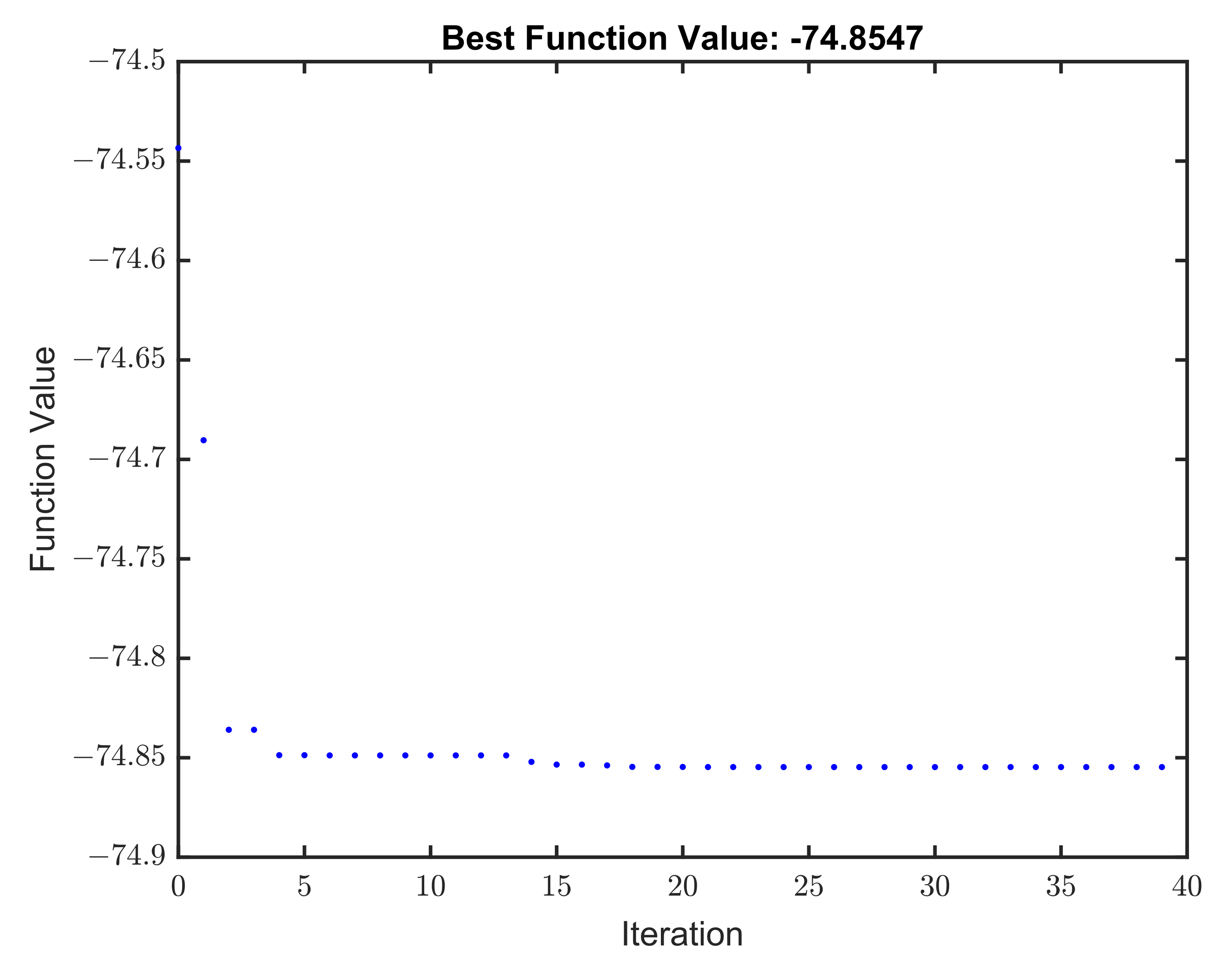
2.4.4. Particle Swarm Optimization (PSO)

A population-based optimization approach with naturalistic inspiration is the particle swarm optimization method. The same as genetic algorithms and other optimization techniques of a similar nature, it is a wholly stochastic process. This algorithm replicates the movement of particles, such as the swarming or shoaling of a school of fish, the flying motion of a flock of birds or the schooling of insects. In a similar way, the swarm of potential solutions “wings” in the direction of the best solution.
Due to its reputation as one of the most promising, nature-inspired algorithms, particle swarm optimization is often applied in a wide range of scientific applications. This class of optimization technique is significantly well liked because of how easily it can be applied to a variety of problems.
PSO is one of several optimization strategies that have been chosen for this work due to some of its benefits over other approaches, including:
  • The PSO algorithm is simple to implement, making it applicable to both engineering and scientific research problems;
  • It has fewer parameters to be adjusted;
  • PSO is more efficient since only the most optimistic particle may pass information to the other particles over the evolution of generations, and, therefore, the optimization procedure moves quite quickly to better fitness values.
The MATLAB optimization toolbox package contains the algorithm employed in the current work. The size of the problem, the computational cost and the required accuracy are all taken into consideration while choosing the algorithm’s parameters by trial and error. Specifically, the algorithm’s self-adjustment and social-adjustment parameters are set to 1.49, the maximum number of iterations to 250, the inertia range to [0.1, 1.1], the stall iteration limit to 20 and the swarm size to 100 particles.
In Figure 4, the optimization procedure is displayed. At each iteration, the MATLAB code that we developed for the FE model implementation is executed to calculate the objective function of Equation (53) needed by the optimization process. As the first step of the optimization procedure, the PSO parameters (number of design variables, swarm size, maxiter, lower and upper bounds of the design variables) are defined. At each step, the algorithm evaluates the objective function at each particle. After this evaluation, the algorithm decides on the new velocity of each particle. The particles move, then the algorithm reevaluates. The maximum number of iterations or a sufficient level of fitness serve as the convergence criteria. As long as the criterion is not satisfied, the algorithm continues to evolve the particles population. Finally, the optimal solution is obtained.

3. Results and Discussion

This section presents the numerical results of the optimal design for the cantilever composite beam seen in Figure 1. Thomas et al. [24] previously studied this beam for single-mode shunt damping. The host beam is made of aluminum, and the piezoceramics are PIC151 and are placed 0.5 mm from the fixed end. The material and geometric properties of the structure are given in Table 2. In this study, the second and third mode of the cantilever beam are damped using the multimode resonant shunt shown in Figure 3b. The reason for only addressing the second and third modes is that, due to the position of the piezoelectric patch, these modes have greater authority than other structural modes. For the determination of the frequency response, the proposed FE model is used, and the harmonic force is applied at the tip of the beam. The system response is determined at the same position.
Three different optimization problems are studied, as already discussed in Section 4. In each problem, the particle swarm optimization method is applied with the number of particles in the swarm set to be 150 and the maximum number of iterations to be 250. The numerical experiment is carried out in the Windows 10 Pro environment running MATLAB 2019b. The computer processor is 11th Gen Intel(R) Core (TM) i7-11370H @ 3.30 GHz, and the RAM is 16.00 GB. Initially, the parameters of the model 1 are chosen with the trial-and-error method by taking into account the commercial availability of the electrical components, the size of the problem and the desired accuracy. The upper and lower bounds of the design variables are given in Table 3.

3.1. Validation versus Results from a Cantilever Beam Connected to a R L Shunt Circuit

The developed finite-element model is verified with the results of [24]. For comparison reasons, a concentrated mass of 4.2 g at the tip of the beam is added to model the magnet used in the non-contact electromagnetic driving system. The dynamic analysis of the beam is performed, and the first three flexural modes are presented in Table 4. Comparing the results from the present FE model with that of the finite-element computations and experiments obtained in [24], an excellent agreement is obtained.
In addition, the effect of an R L shunt circuit connected in series with the upper and lower piezoelectric patch, as presented in [24], is studied next. Using the values of R = 7900 Ω and L = 21.8 H , the driving point FRF modulus at the tip of the beam (i.e., the response at the tip for an excitation at the same point) from the present finite-element formulation as well as from the formulation of [24] is shown in Figure 5. Again, an excellent agreement is obtained between the two formulations.
The results clearly illustrate the high accuracy and reliability of the present FE formulation for frequency response analysis of piezoelectric composite beams, and, therefore, this numerical analysis can be readily integrated efficiently with the PSO algorithm to provide optimal solutions to the optimization problems.

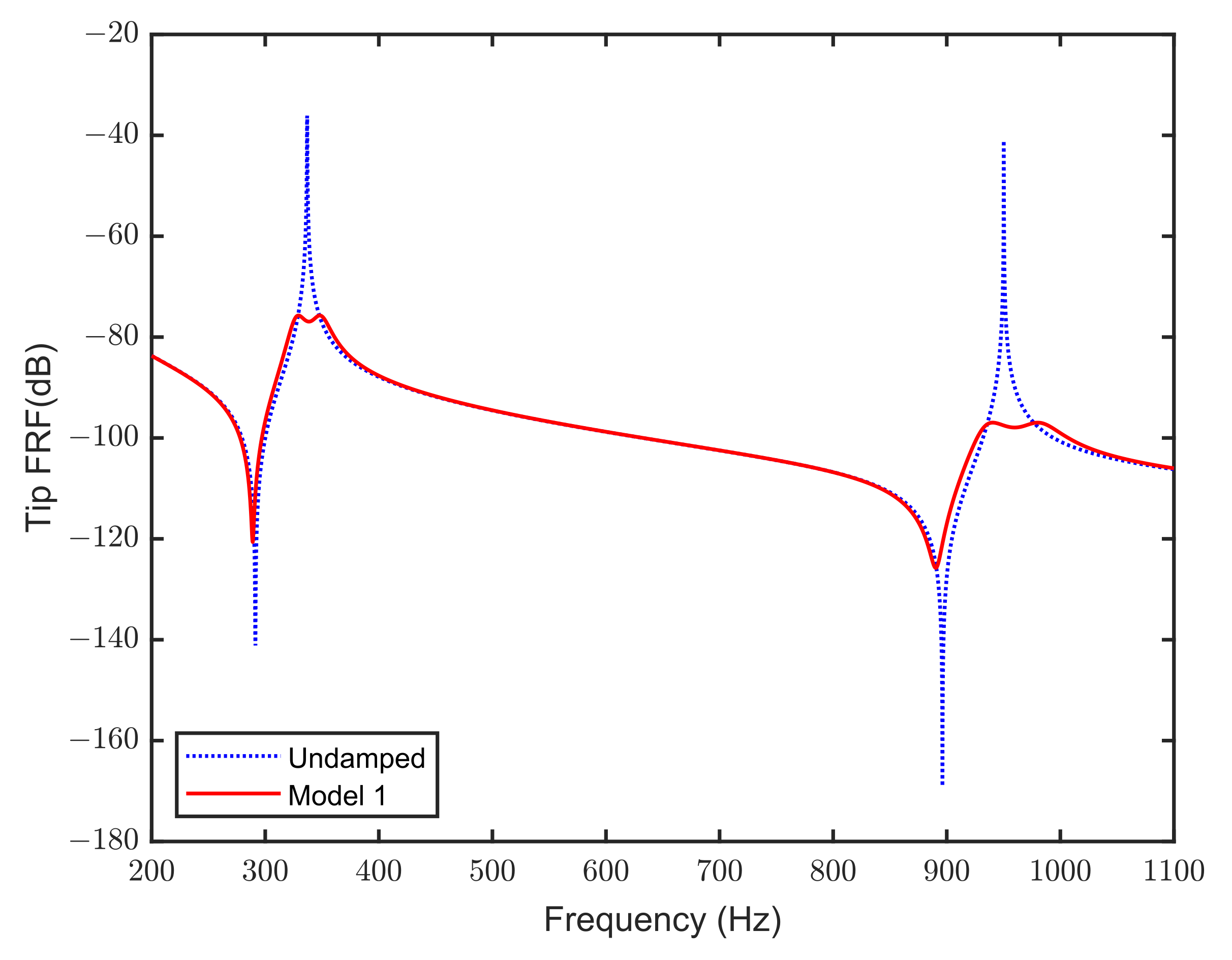
3.2. Solution of Optimization Problem: Model 1

The optimization problem in Equation (54) is addressed at this stage by considering the resistance values R i , the capacitances C i and the inductance values of the shunt-damping sub-branch L ˜ i as the design variables. The inductance values L ^ i of the current-flowing branch are given by Equation (31), while the inductances of the simplified shunt circuit in Figure 3b are obtained as L i = L ^ i + L ˜ i . The problem is solved with the limit values given in Table 3. The optimal values of the electrical parameters of the simplified shunt circuit are given in Table 5.
To justify the H norm optimization technique, the magnitude frequency response of the tip displacement, before and after shunt damping, is presented in Figure 6. It is observed that the damped FRF exhibits two peaks of equal amplitude around each of the second and the third natural frequencies, which are comparatively low with respect to the uncontrolled structure (when the transducer is either short or open circuited). Indeed, the resonant amplitudes for the second and third modes are reduced by 39.61 dB and 55.92 dB, respectively.
Figure 7 shows the convergence of the particle swarm optimization algorithm for model 1. As can be seen from Figure 7, the process converges after generation 45, when the fitness function remains quasi constant. It takes about 1 h to carry out the 105 iterations. In addition, the algorithm stops before the maximum iteration is reached, since the relative changes in objective function are less than the tolerance (10−6).

3.3. Solution of Optimization Problem: Model 2

In this case, the optimization problem described by Equation (55) is solved by setting the lower R L and upper R U bounds for the resistance values to be the same as in model 1 (see Table 3). The capacitance values C i are chosen to be 10% of the inherent capacitance of the piezoelectric patch, and the inductance values L i are given by Equation (35). The optimal values of the resistance variables found by the PSO algorithm are R 2 = 12.29   k Ω and R 3 = 4.02   k Ω . Figure 8 shows the magnitude of the tip FRF, before and after shunt damping, using the method proposed by Behrens et al. [16] (model 2). For comparison reasons, the corresponding FRF of the damped system using the proposed method (model 1) is also illustrated simultaneously in this figure. It is obvious from Figure 8 that the proposed method provides greater amplitude reduction in both target modes. Indeed, the FRF amplitude reduction of the second mode is 25.47 dB, i.e., 35.69% lower compared with that of model 1 (39.61 dB). Additionally, the FRF amplitude reduction of the third mode is 47.08 dB, i.e., 15.81% lower compared with that of model 1 (55.92 dB). The overall parameters of the shunt circuit for model 2 are shown in Table 6. It can be observed that the required inductance values for the convectional current-flowing method (model 2) are considerably large, especially those corresponding to low-frequency modes. In comparison with the optimal inductance values of model 1, it follows that the suitable choice of the capacitance values C i via the proposed optimization method significantly reduces the inductive requirements.
Figure 9 shows the iteration process of optimization. It can be seen from the figure, that the process converges after generation 15, when the fitness function remains quasi constant. It takes about 17 min to carry out the 39 iterations. In addition, the algorithm stops before the maximum iteration is reached, since the relative changes in objective function are less than the tolerance (10−6).

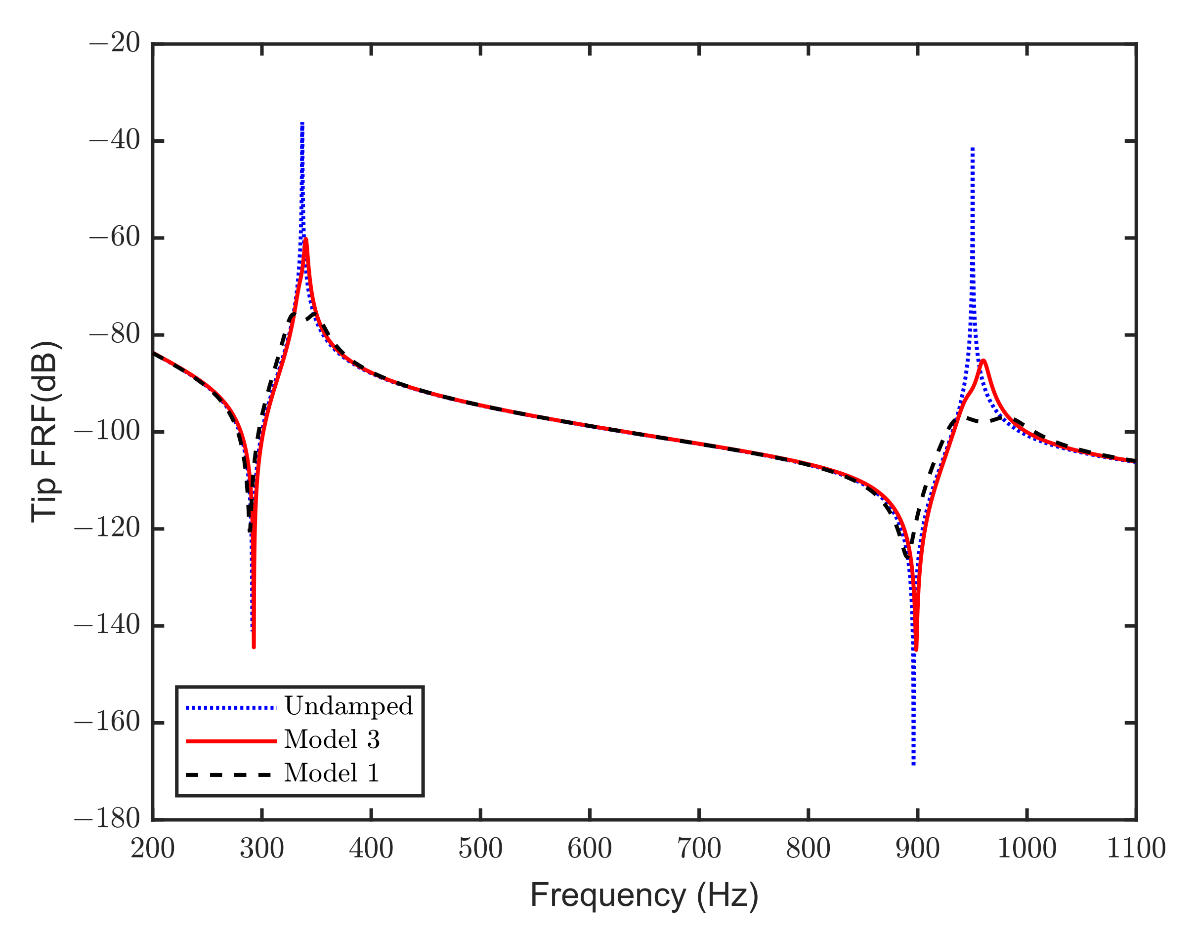
3.4. Solution of Optimization Problem: Model 3

Finally, the optimization problem defined by Equation (56) is solved with the resistance values R i and the capacitance values C i considered as design variables. Given the capacitances, the inductance values L i of the simplified shunt circuit are determined by Equation (35). The lower and upper limits for the resistances and the capacitances vary, the same as in model 1 and are given in Table 3. The optimal values of the design variables, along with the calculated inductances, are given in Table 7. As we can see, the required inductance values for this model are even larger relative to model 2 and considerably larger compared to the ones of model 1. The magnitude frequency response of the tip displacement, before and after shunt damping, are presented in Figure 10. For the purpose of comparison, the corresponding magnitude frequency response of model 1 is also illustrated simultaneously in this figure. It can be observed from this figure that the amplitude reduction for model 1 is higher than that of model 3. It means that model 1 yields better results than the model 3. Using the values of the shunt circuit from Table 7, the resonant amplitudes for the second and third modes are reduced by 24.07 dB and 44.22 dB, respectively. Compared with the corresponding reduction obtained when the shunt system is tuned according to the proposed method of model 1, these reductions are obvious lower.
Figure 11 shows the iteration process of optimization. It can be seen from the figure, that the process converges after generation 5, when the fitness function remains quasi constant. It takes about 15 min to carry out the 38 iterations. Again, the algorithm stops before the maximum iteration is reached, since the relative changes in objective function are less than the tolerance (10^-6).

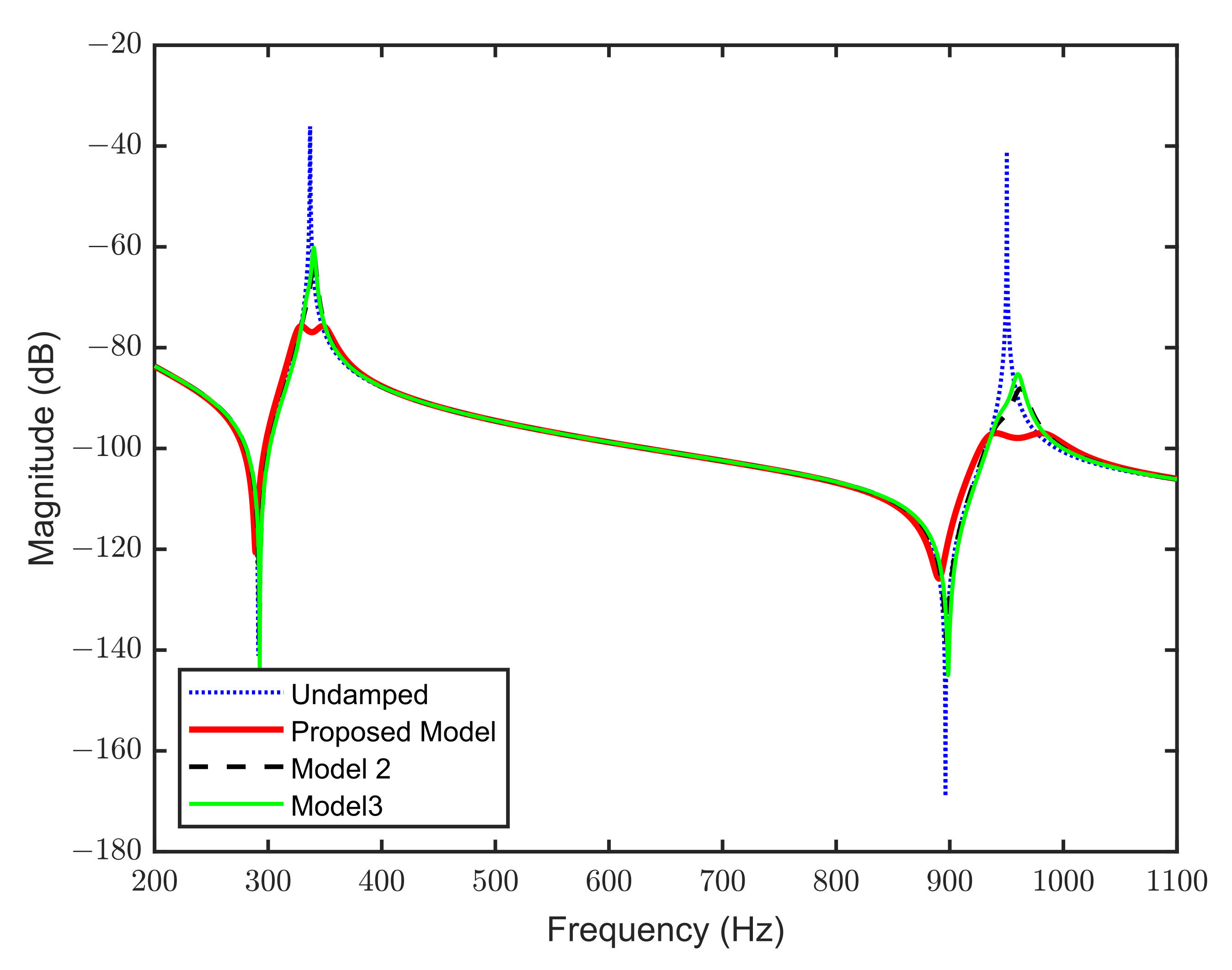
3.5. Comparison between the Three Models

An overall comparison between the three models is given in this section. For this reason, the tip FRFs using optimal solutions of all models are illustrated simultaneously in Figure 12. It can be observed from this figure that the optimal solution of the proposed model 1 gives greater amplitude reduction than both the other models. This means that the proposed model 1 yields better results than all the other models. The same conclusion can be obtained by comparing the amplitude reduction for the second and the third mode for all models given in Table 8.
Additionally, in comparison to model 2, the numerical results demonstrate the beneficial impact of the third design variable, “inductance of the shunting branches”. Another benefit of the approach introduced in model 1 is that of reducing the required inductance values of the multimode shunt circuits. Indeed, comparing the inductance values required for shunt damping control in all models (see Table 5 and Table 6), the total inductances in model 1 have the lower values. It seems that considering the capacitances as design variables to be determined and tuning their values via optimization method is an alternative way to reduce the inductance requirements of piezoelectric shunt-damping systems [16]. However, in contrast to the method of [16], the proposed approach is not performed at the expense of damping performance.

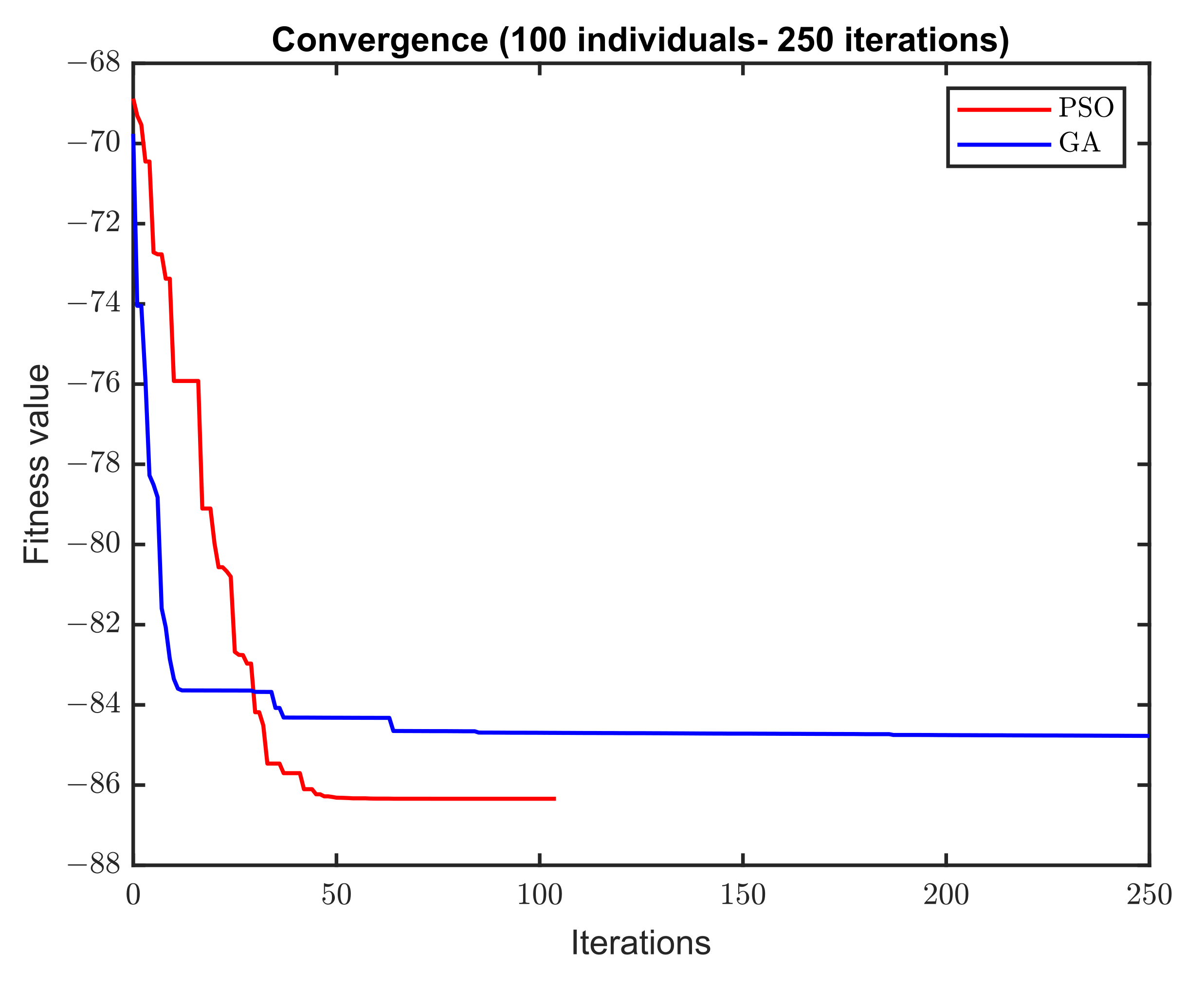
3.6. A Comparison between PSO and GA Algorithms

In this section, a comparison between the proposed PSO method and GA algorithm is performed in order to demonstrate the capability of the proposed PSO method to improve the performance of shunt-damping circuits. Each algorithm is run 10 times with the same number of particles/population (100) and the same number of maximum iterations/generations (250). The remaining parameters for the GA algorithm are the default parameters of the GA solver in MATLAB, while, for PSO, the same parameters as mentioned above are used.
Table 9 and Table 10 show the best fitness value found, the total time (in s) the iterations/generations executed for the algorithm take in order to start to converge, the total number of iterations and the total function evaluations required to find the optimal solution for both algorithms in each run time. Based on the results tabulated in Table 8 and Table 9, most best fitness values found by PSO are lower than the ones found by GA in most of the 10 test runs. In fact, 70% of the fitness values reached by PSO are lower than −86, a value that is never reached by GA. For PSO, the lowest fitness value of −86.34 is reached with 10,600 objective function evaluations. Nevertheless, GA reaches its best value −84.77 using a computational effort relative to 23,855 evaluations, as shown in Table 8 and Table 9. Additionally, it is observed that the average time required by PSO to find the optimal circuit design (in 10 test runs) is shorter compared to GA, which shows that PSO can perform faster than GA.
Figure 13 shows a comparison of the PSO and GA methodologies’ convergence during the search process of the optimal parameters for the test run (execution) with the best fitness value. It is clear from this figure that PSO converges at a faster rate (around 45 iterations) than GA (around 232 generations). Another interesting outcome of this figure is that, in GA, although the best solution is improved relatively fast in the first 70 iterations, in the remaining iterations, it is trapped in a local optimum, which is worster from the solution found using the PSO. Thus, this comparison demonstrates the capability of PSO to reach better values for this kind of problem and exert less computational effort to reach the “optimum” when compared to GA. Nevertheless, a more comprehensive study is needed to establish this statement, which is out of the scope of this study.

4. Conclusions

This work provides a new design optimization approach for enhancing multimode vibration damping of composite beam structures. A modification of the “current-flowing” shunt circuit [15] for controlling multimode vibration in a piezoelectric laminate beam is used. The proposed method is based on considering the capacitor and inductor values of each shunting branch as new design variables along with the resistor values. The optimization is performed for the minimum H norm of the piezoelectric composite beam using a PSO algorithm. A two-mode shunt circuit is designed and simulated for a cantilever piezo laminated beam. Two additional models with different combinations of variables are investigated; model 2 considers only the resistances of the shunt circuit as design variable, and model 3 considers both resistances and capacitances. Frequency response analysis is conducted by the finite-element method using super-convergent beam elements. The obtained optimal solutions are presented and discussed. The overall results show that the proposed approach of model 1 improves the multimode shunt damping and gives the highest peak amplitude reduction of 39.61 dB for the second mode and 55.92 dB for the third mode. Another benefit of the approach introduced in model 1 is that of the reduction of the required values for the inductors without any expense in the damping performance. Finally, a comparison of the proposed PSO method with the GA algorithm is performed, which demonstrates the capability of PSO to reach better values for this kind of problem and exert less computational effort to reach the “optimum”.

Author Contributions

Conceptualization, K.M., G.K.T. and G.E.S.; methodology, G.A.F. and N.A.A.; software, K.M., G.K.T., G.A.F., N.A.A. and G.E.S.; validation, K.M. and G.K.T.; formal analysis, N.A.A.; investigation, K.M., G.A.F. and G.E.S.; resources K.M., G.A.F. and G.E.S.; data curation, K.M. and G.A.F.; writing—original draft preparation, G.A.F. and N.A.A.; writing—review and editing, K.M., N.A.A. and G.E.S.; visualization, G.A.F. and N.A.A.; supervision, G.E.S. All authors have read and agreed to the published version of the manuscript.

Funding

This research received no external funding.

Institutional Review Board Statement

Not applicable.

Informed Consent Statement

Not applicable.

Data Availability Statement

Not applicable.

Conflicts of Interest

The authors declare no conflict of interest.

References

  1. Yan, B.; Wang, K.; Hu, Z.; Wu, C.; Zhang, X. Shunt Damping Vibration Control Technology: A Review. Appl. Sci. 2017, 7, 494. [Google Scholar] [CrossRef]
  2. Marakakis, K.; Tairidis, G.K.; Koutsianitis, P.; Stavroulakis, G.E. Shunt Piezoelectric Systems for Noise and Vibration Control: A Review. Front. Built Environ. 2019, 5, 64. [Google Scholar] [CrossRef]
  3. Forward, R.L. Electronic Damping of Vibrations in Optical Structures. Appl. Opt. 1979, 18, 690. [Google Scholar] [CrossRef] [PubMed]
  4. Hagood, N.W.; von Flotow, A. Damping of Structural Vibrations with Piezoelectric Materials and Passive Electrical Networks. J. Sound Vib. 1991, 146, 243–268. [Google Scholar] [CrossRef]
  5. Park, C.H. Dynamics Modelling of Beams with Shunted Piezoelectric Elements. J. Sound Vib. 2003, 268, 115–129. [Google Scholar] [CrossRef]
  6. Pietrzko, S.; Mao, Q. Control of Structural Sound Radiation and Vibration Using Shunt Piezoelectric Materials. JSDD 2011, 5, 752–764. [Google Scholar] [CrossRef] [Green Version]
  7. Tairidis, G.K.; Marakakis, K.; Koutsianitis, P.; Foutsitzi, G.; Deü, J.F.; Stavroulakis, G.E.; Ohayon, R. Vibration Control of Smart Composite Plates Using Shunted Piezoelectric Elements. In Proceedings of the 9th ECCOMAS Thematic Conference on Smart Structures and Materials, SMART 2019, Paris, France, 8–12 July 2019. ⟨hal-03179056⟩. [Google Scholar]
  8. Raze, G.; Dietrich, J.; Lossouarn, B.; Kerschen, G. Modal-Based Synthesis of Passive Electrical Networks for Multimodal Piezoelectric Damping. Mech. Syst. Signal Process. 2022, 176, 109120. [Google Scholar] [CrossRef]
  9. Bo, L.D.; He, H.; Gardonio, P.; Li, Y.; Jiang, J.Z. Design Tool for Elementary Shunts Connected to Piezoelectric Patches Set to Control Multi-Resonant Flexural Vibrations. J. Sound Vib. 2022, 520, 116554. [Google Scholar] [CrossRef]
  10. Hollkamp, J.J. Multimodal Passive Vibration Suppression with Piezoelectric Materials and Resonant Shunts. J. Intell. Mater. Syst. Struct. 1994, 5, 49–57. [Google Scholar] [CrossRef]
  11. Wu, S.-Y. Method for Multiple Mode Piezoelectric Shunting with Single PZT Transducer for Vibration Control. J. Intell. Mater. Syst. Struct. 1998, 9, 991–998. [Google Scholar] [CrossRef]
  12. Behrens, S.; Reza Moheimani, S.O. Optimal Resistive Elements for Multiple Mode Shunt Damping of a Piezoelectric Laminate Beam. In Proceedings of the 39th IEEE Conference on Decision and Control (Cat. No.00CH37187), Sydney, Australia, 12–15 December 2000; IEEE: Sydney, NSW, Australia, 2000; Volume 4, pp. 4018–4023. [Google Scholar]
  13. Behrens, S.; Moheimani, S.O.R. Current Flowing Multiple-Mode Piezoelectric Shunt Dampener; Agnes, G.S., Ed.; SPIE: San Diego, CA, USA, 2002; pp. 217–226. [Google Scholar]
  14. Behrens, S.; Moheimani, S.O.R.; Fleming, A.J. Multiple Mode Passive Piezoelectric Shunt Dampener 1. IFAC Proc. Vol. 2002, 35, 161–166. [Google Scholar] [CrossRef]
  15. Behrens, S.; Moheimani, S.O.R.; Fleming, A.J. Multiple Mode Current Flowing Passive Piezoelectric Shunt Controller. J. Sound Vib. 2003, 266, 929–942. [Google Scholar] [CrossRef]
  16. Fleming, A.J.; Behrens, S.; Moheimani, S.O.R. Reducing the Inductance Requirements of Piezoelectric Shunt Damping Systems. Smart Mater. Struct. 2003, 12, 57–64. [Google Scholar] [CrossRef]
  17. Fleming, A.J.; Behrens, S.; Reza Moheimani, S.O. Optimization and Implementation of Multimode Piezoelectric Shunt Damping Systems. IEEE/ASME Trans. Mechatron. 2002, 7, 87–94. [Google Scholar] [CrossRef]
  18. Jeon, J.-Y. Passive Vibration Damping Enhancement of Piezoelectric Shunt Damping System Using Optimization Approach. J. Mech. Sci. Technol. 2009, 23, 1435–1445. [Google Scholar] [CrossRef]
  19. Raze, G.; Dietrich, J.; Kerschen, G. Tuning and Performance Comparison of Multiresonant Piezoelectric Shunts. J. Intell. Mater. Syst. Struct. 2022, 33, 2470–2491. [Google Scholar] [CrossRef]
  20. Raze, G.; Dietrich, J.; Kerschen, G. Passive Control of Multiple Structural Resonances with Piezoelectric Vibration Absorbers. J. Sound Vib. 2021, 515, 116490. [Google Scholar] [CrossRef]
  21. Toftekær, J.F.; Høgsberg, J. Multi-Mode Piezoelectric Shunt Damping with Residual Mode Correction by Evaluation of Modal Charge and Voltage. J. Intell. Mater. Syst. Struct. 2020, 31, 570–586. [Google Scholar] [CrossRef]
  22. Wu, S. Piezoelectric Shunts with a Parallel R-L Circuit for Structural Damping and Vibration Control. In Proceedings of the 1996 Symposium on Smart Structures and Materials, San Diego, CA, USA, 25–29 February 1996; SPIE: Bellingham, WA, USA, 1996; Volume 2720, pp. 259–269. [Google Scholar] [CrossRef]
  23. Thomas, O.; Deü, J.-F.; Ducarne, J. Vibrations of an Elastic Structure with Shunted Piezoelectric Patches: Efficient Finite Element Formulation and Electromechanical Coupling Coefficients. Int. J. Numer. Meth. Engng 2009, 80, 235–268. [Google Scholar] [CrossRef]
  24. Foutsitzi, G.; Gogos, C.; Antoniadis, N.; Magklaras, A. Multicriteria Approach for Design Optimization of Lightweight Piezoelectric Energy Harvesters Subjected to Stress Constraints. Information 2022, 13, 182. [Google Scholar] [CrossRef]
  25. Foutsitzi, G.; Gogos, C.; Hadjigeorgiou, E.; Stavroulakis, G. Actuator Location and Voltages Optimization for Shape Control of Smart Beams Using Genetic Algorithms. Actuators 2013, 2, 111–128. [Google Scholar] [CrossRef]
  26. Reddy, J.N. Mechanics of Laminated Composite Plates and Shells: Theory and Analysis, 2nd ed.; CRC Press: Boca Raton, FL, USA, 2004; ISBN 978-0-8493-1592-3. [Google Scholar]
  27. Foutsitzi, G.; Hadjigeorgiou, E.; Gogos, C.; Stavroulakis, G.E. Modal Shape Control of Smart Composite Beams Using Piezoelectric Actuators. In Proceedings of the 10th HSTAM International Congress on Mechanics, Chania, Greece, 25 December 2013. [Google Scholar]
  28. Gripp, J.A.B.; Rade, D.A. Vibration and Noise Control Using Shunted Piezoelectric Transducers: A Review. Mech. Syst. Signal Process. 2018, 112, 359–383. [Google Scholar] [CrossRef]
  29. Caruso, G. A Critical Analysis of Electric Shunt Circuits Employed in Piezoelectric Passive Vibration Damping. Smart Mater. Struct. 2001, 10, 1059–1068. [Google Scholar] [CrossRef]
  30. Beck, B.S.; Cunefare, K.A.; Collet, M. The Power Output and Efficiency of a Negative Capacitance Shunt for Vibration Control of a Flexural System. Smart Mater. Struct. 2013, 22, 065009. [Google Scholar] [CrossRef]
  31. De Marneffe, B.; Preumont, A. Vibration Damping with Negative Capacitance Shunts: Theory and Experiment. Smart Mater. Struct. 2008, 17, 035015. [Google Scholar] [CrossRef] [Green Version]
  32. Berardengo, M.; Manzoni, S.; Vanali, M.; Bonsignori, R. Enhancement of the Broadband Vibration Attenuation of a Resistive Piezoelectric Shunt. J. Intell. Mater. Syst. Struct. 2021, 32, 2174–2189. [Google Scholar] [CrossRef]
Figure 1. A cantilever beam with a piezoelectric patch connected to a shunt-damping network.
Signals 03 00050 g001
Figure 2. Current-flowing shunt circuit for multimode damping.
Signals 03 00050 g002
Figure 3. (a) A single-shunt circuit for two-mode current-flowing control. (b) Simplified shunt circuit.
Signals 03 00050 g003
Figure 4. Flowchart of the optimization procedure.
Signals 03 00050 g004
Figure 5. Beam tip FRF with RL shunt tuned on mode 2: undamped response (blue ---), damped—present FE (red), damped FE of Thomas et al., 2009 [24] (black).
Signals 03 00050 g005
Figure 6. Simulated frequency response: undamped response (blue ---), damped response—model 1 (red).
Signals 03 00050 g006
Figure 7. Iteration process of the fitness function using PSO—model 1.
Signals 03 00050 g007
Figure 8. Simulated frequency response: undamped response (blue ---), damped response—model 2 (red).
Signals 03 00050 g008
Figure 9. Iteration process of the fitness function using PSO—model 2.
Signals 03 00050 g009
Figure 10. Simulated frequency response: undamped response (blue ---), damped response—model 3 (red).
Signals 03 00050 g010
Figure 11. Iteration process of the fitness function using PSO—model 3.
Signals 03 00050 g011
Figure 12. Simulated frequency response of the three models.
Signals 03 00050 g012
Figure 13. Convergence of the best fitness for PSO and GA optimization techniques.
Signals 03 00050 g013
Table 1. Summary of the various passive damping methods investigated.
ReferencesSingle-Mode ControlMulti-
Mode Control
Single
Piezo
Patch
Multiple
Piezo
Patches
PSOOther
Optimization Approach
Current-Flowing
Method
Other
Shunt Method
Forward (1979) [3]
Hagood et al. (1991) [4]
Park (2003) [5]
Pietrzko et al. (2011) [6]
Tairidis et al. (2019) [7]
Raze et al. (2022) [8]
Bo et al. (2022) [9]
Hollkamp (1994) [10]
Wu (1998) [11]
Behrens et al. (2000) [12]
Behrens et al. (2002) [13,14,15]
Fleming et al. (2003) [16,17]
Jeon (2009) [18]
Raze et al. (2022) [19]
Raze et al. (2020) [20]
Toftekær et al. (2020) [21]
Wu (1996) [22]
Table 2. Geometric and material parameters of the compound structure.
ParameterBeamPZT
Length L (mm)17025
Width b (mm)2020
Thickness h (mm)20.5
Young’s modulus E (GPa)7266.7
Shear modulus G 12 (GPa)27.4825.46
Poisson’s ratio v 12 0.310.31
Density ρ   ( Kg / m 3 )28008500
Piezoelectric constant e ˜ 31 ( C / m 2 )-−14
Dielectric constant ξ ¯ 33 (nF/m)-2068 ε 0
ε 0 = 8.854 × 10 12 F/m is the free space permittivity.
Table 3. The limits of the design variables.
VariableMinimal ValueMaximum Value
R 2   k Ω 030
R 3   k Ω 030
C 2   μ F 10−81
C 3   μ F 10−81
L ˜ 2   H 120
L ˜ 3 H 120
Table 4. The first three natural frequencies (Hz) of the piezoelectric composite beam.
ModesShort-Circuit Frequencies (Hz)Open-Circuit Frequencies (Hz)
FE [24]Exp. [24]Present FEFE [24]Exp. [24]Present FE
148.9651.6448.9649.4252.1749.2
2337.1337.0336.9340.7340.2338.68
3951.8936.3950.23960.6940.0954.64
Table 5. Shunt parameters for model 1.
ParameterValue
R 2   k Ω 1.40
R 3   k Ω 2.36
C 2   μ F 1
C 3   μ F 0.0083
L ˜ 2   H 7.43
L ˜ 3   H 1.68
L 2   H 7.68
L 3   H 5.06
Table 6. Shunt parameters for model 2.
ParameterValue
R 2   k Ω 12.29
R 3   k Ω 4.02
C 2   nF 1.83
C 3   nF 1.83
L 2   H 134.07
L 3   H 16.85
Table 7. Shunt parameters for model 3.
ParameterValue
R 2   k Ω 16.34
R 3   k Ω 5.43
C 2   μ F 0.001
C 3   μ F 0.001
L 2   H 235.36
L 3   H 29.59
Table 8. Amplitude reduction (dB).
Model 1Model 2Model 3
Mode 239.6025.4724.07
Mode 355.9247.0844.22
Table 9. Fitness, computation time and iterations of GA.
Number of RunsBest FitnessTime (s)Total
Iterations
Function Evaluations
1−84.778326.05325023,855
2−70.56513.6925023,855
3−80.967823.0225023,855
4−69.333644.8011110,650
5−83.347231.3625023,855
6−70.727508.0425023,855
7−70.244252.6518918,060
8−69.62168.00726945
9−80.77050.1725023,855
10−83.587220.2825023,855
Avg Total−76.3746173.81212.220,264
Table 10. Fitness, computation time and iterations of PSO.
Number of RunsBest FitnessTime (s)Total
Iterations
Function Evaluations
1−70.194277.7511211,300
2−86.343897.5110510,600
3−86.236653.8223023,100
4−86.233428.3413213,300
5−70.192256.21909100
6−86.188431.5925025,100
7−86.215426.7517317,400
8−86.238045.1725025,100
9−70.193946.7014214,300
10−867613.4925025,100
Avg Total−81.3995397.73173.417,440
Publisher’s Note: MDPI stays neutral with regard to jurisdictional claims in published maps and institutional affiliations.

