1. Introduction
Air pollution is responsible for a plethora of diseases, including lung disease, chronic respiratory disease, and stroke [
1]. Prevention and control of air pollution is a primary concern of governments and research institutions, due to the severity of the consequences. In [
2], studies of air pollution include the use of prediction systems and management of prevention. The idea is to determine policy-making by studying pollution metrics adequately and appropriately. Moreover, spatial characterisation of air pollution is of the utmost importance [
3].
Emissions in the transport domain constitute a huge factor in air quality. Specifically, ship emissions including SOx, NOx, PM, and CO have a key impact on coastal atmospheric pollution [
4]. In particular, in terms of air quality in ports, ships play an important role in the increase of air pollution. Because ships’ energy is coming from heavy fuel oil (HFO), when they are docked in ports, activities such as refrigeration, cargo handling, and air-conditioning come at the expense of energy spent and compromised air quality [
5]. The International Maritime Organisation (IMO) set some key guidelines for ship actions that minimise the environmental pollution footprint [
6]. Furthermore, it is thus imperative to address all aspects of air pollution in ports, including that of external container trucks. In [
7] the authors state that external container trucks produce more pollution than cargo-related equipment.
Ports occasionally reside close to residential areas. Depending on the season, the wind may circulate and lead to pollution particles in the residential areas, which essentially increase air pollution. The same applies with fresh air [
8]. Hence, we have to monitor the air quality in the port because pollution can be evident and extended even to the residential areas. As such, in order to be able to achieve reduced air pollution, it is necessary to have the means to perform environmental monitoring as well as estimation [
9], forecasting [
10], and prediction [
11] in the port area. A number of studies are available, whereby monitoring is taking place in port areas [
12,
13,
14,
15].
In conjunction with monitoring, machine-learning methods have been employed on several occasions, in order to classify and predict the impact of emissions in ports and nearby residential areas, as well as other parameters, such as truck-traffic volume and freight transportation management, which will be presented in the most recent related work.
Machine learning is a branch of artificial intelligence (AI) that provides systems the capability to learn and improve from experience in an automated manner, without being explicitly programmed. Machine learning deals with the implementation of computer programs that can access data and use it to learn for themselves. One of the most well-known machine-learning methods is the neural network. Neural networks [
16] have been used in a number of research works for atmospheric evaluation and ar quality [
17,
18,
19,
20,
21]. Here we use the LSTM networks [
22], which is a good candidate for the prediction of the port’s CO values. In particular, we use a univariate LSTM, which is a special kind of recurrent neural network (RNN) [
23] with additional features to memorize the sequence of data.
LSTM systems were outlined particularly to overcome the long-term dependency issue confronted by repetitive neural systems (RNNs). LSTMs have input associations which make them diverse to more conventional feedforward neural systems. This property empowers LSTMs to handle whole arrangements of information (e.g., time arrangement) without treating each point within the grouping freely, potentially holding valuable information about past data within the arrangement to assist with the handling of unused information focuses. As a result, LSTMs are especially great at handling arrangements of information such as content, discourse, and common time series.
In particular, the RNN structure resembles the hidden Markov model (HMM). The main difference is the way that the parameters are calculated and created. One of the LSTM advantages is the insensitivity to the gap length. RNN and HMM focus on the hidden state before sequence. In the case that we wish to make a prediction of a sequence after 1000 intervals instead of 10, the model will forget the starting point; however, LSTM has a memory to perform this task. A detailed description of the LSTM and an application regarding field data forecasting can be found in [
24]. In addition, the original LSTM is very slightly not enough in explaining the relationship of the input and output of the networks. In [
25], to solve this problem, the attention-based mechanism is inserted into LSTM. Moreover, in [
26] local air pollution measurements close to main streets, which reside on small Internet of Things (IoT) devices in combination with artificial intelligence algorithms were used for prediction of PM
and PM
concentration. Another work based on the ARIMA model is in [
27], whereby the trend analysis as well forecast of PM2.5 in Fuzhou, China has been undertaken.
In this paper, we collect data from a set of environmental sensors, which form a wireless environmental sensor located in the broader area of the port of Igoumenitsa in Greece. The station measures the most important pollutants including the CO in the port. We analyse the CO measurements at 6-h intervals for the entire dataset. We show that there exists an abnormal rise in values. Thereafter, we transform the dataset to a moving average values dataset, in order to reduce extremely high values. The moving average is a popular method by which to transform a dataset to a smoother problem, in terms of the values used for the prediction phase. Moving average smoothing is a naive and effective technique in time series forecasting. It can be used for data preparation, feature engineering, and even directly for making predictions. Importantly, we utilise machine learning and especially LSTM to show the predicted outcome of the collected values from the port by using different batches of the procedure.
The main contributions of this paper are the following.
We produce a dataset whereby the CO is measured at a fixed period of time, in order to utilise it in the LSTM and ARIMA models.
We devise an LSTM model for values prediction, and we show that the results are close to the actual values when the batch number is 7000.
We perform a comparison with the ARIMA model, and show that the LSTM accomplishes similar results to the ARIMA, with the ARIMA being better in the forecasting.
The remainder of this paper is as follows:
Section 2 gives the related work,
Section 3 provides details about the wireless station used,
Section 4 provides the data description,
Section 5 gives the method used for the prediction of the CO,
Section 6 presents the results of the algorithms, and
Section 7 provides the conclusions of this work.
2. Related Work
This section essentially summarises similar works that utilised ML models to accomplish air pollution monitoring in ports and surrounding areas. A number of cases have been identified that show the necessity of the monitoring procedure in this particular part of a city because ports often reside within city limits and can contribute to air pollution. Truck traffic is also given because in large ports it can be a source of pollution due to the fact that they load and unload in the port, often carrying containers and other goods. In the future, data from trucks will be added to the proposed forecasting model to provide a multivariate approach of CO pollution prediction.
In [
28], the authors suggest the use of wireless sensors to perform air pollution monitoring. In addition, the system is given prediction capabilities, which consider conditions of the local climate within a city. An investigation is undertaken which shows that there is a difference in measurements of the microclimate at a street level, which imposes a change in the prediction accuracy. Thus, the sensors are equipped with mini low-power artificial neural networks (ANN)s, which are trained from their local environment, rather than doing so from a base station.
In [
29] the authors have used a machine-learning (ML) model, in order to proceed with the prediction of air quality in the city of Barcelona. To this end, weather and pollutant concentrations were gathered by the use of networks in the area of the city. The tool which is described has been proven to exhibit better performance than the CALIOPE Urban v1.0 platform, with respect to predictive capabilities of local
concentration levels. This paper proposed the utilisation of metrics including the mean squared and absolute errors to show the predictive accuracy. For the dataset that was used and for all stations and pollutants, the best performance was shown to be accomplished by using the gradient boosting machine (GBM). In terms of the importance of pollution factors, the research showed that one of the least important predictors was the number of cruise ships in the port, among the work-week day, precipitation, and relative humidity. The most important factors that impacted the pollutant level variability were the time of the year, the time of day, and the intensity of the road traffic. The ML tool also has been used to distinguish and calculate the air-quality level with respect to the overall port activity and due to cruise liners. This task took place using the difference between the observed and predicted pollutant concentrations for several difference values with respect to the actual number of vessels. Results have shown that the liners’ contributions to the worsened air quality around the port of Barcelona is limited compared to that of the overall port operation.
In [
30], the authors present a research work, which aims to show the reduction of unclean production of
emissions of the crane of the port and contributed to clean air gains. Towards achieving this, they studied the Casablanca port of Morocco, and utilised its data regarding the daily energy of eleven RTG cranes that have been collected for a period of two years. The energy consumption has been performed by analysing the data by using a machine-learning tool, namely the regression analysis statistical method, in order to discover the factors impacting the production as well as the degree of the impact. Thereafter the authors treated the factors of high impact by introducing inexpensive strategies towards large investments for clean air. Finally, the authors showed a significant reduction of energy consumption and the reduction of a quite large amount of
emissions per year for the port of Casablanca.
In [
31] the authors provide a complete review of the state-of-the-art ML models and their applications to a number of cases of international freight transportation management (IFTM). Initially, the ML methods are described regarding their functionality. Thereafter, an overview is given about the manner that ML methods are employed, adapted, and applied to different areas of IFTM. These areas include demand forecasting, vehicle trajectory, procedure and asset maintenance, as well as on-time performance prediction. In addition, ML models require data sources in order to be developed. As such, these data sources are investigated towards devising ML models.
In [
32] the authors describe two kernel-based supervised ML models for daily truck traffic in port terminals. The Gaussian processes (GP) and
-support vector machines are considered. This work emphasises the comparison of the aforementioned methods with the multilayer feedforward neural network (MLFNN) model, extensively utilised in prior research works, in order to see the difference in their performance. The model production is accomplished by using the data from Bayport and Barbours Cut container terminals at the port of Houston. The mobility of the trucks is generated during import and export activities at the two terminals. These are examined as different entities; thus, producing four datasets, in order to proceed with the model comparison. When using all four datasets, the two ML models, perform well. Moreover, their prediction outcome exhibits a good comparison with the MLFNN model. Regarding the technical aspects of the ML models, the GP and
-SVM models require less effort in model fitting compared to the MLFNN model. The authors claim that they have good candidates, in order to substitute the MLFNN in port-generated truck-traffic predictions.
3. Wireless Environmental Station
The requirements of the wireless environmental station (WES) essentially constitutes it as a global system for mobile communications-based (GSM) multi-sensor device, used to obtain measurements of pollutants as well as other factors such as the environmental conditions of the monitored area. In particular, the WES should include a power supply and the options to include solar panels, GSM modules, and batteries of NP7-12 (6 batteries) as well as NCR 18650B (30 batteries) types. The environmental sensors available can measure CO, NO, NO
, O
, PM
, PM
, and PM
. The environmental sensors include the temperature, relative humidity, pressure, wind direction, and wind speed. Hence, we selected the RAMP SENSIT devices [
33], which cover the requirements. In
Figure 1, the parts comprising the internal mechanism of the SENSIT device can be seen.
The concept was to deploy a device to the port area of Igoumenitsa, in order to investigate pollution as well as environmental parameters. In
Figure 2 we can see the SENSIT device deployed on a building in the port of Igoumenitsa. The collected data is transmitted to a server, where it is processedand the comma-separated value (csv) file is produced. This file is then processed to be presented in a Web-GIS application, which is a real-time application, showing the parameters in the port area.
Note that the deployment of such a device is a pilot for the deployment of more devices near the port area, in order to monitor the parameters in the broader area of the port, including residential areas, because the port resides very close to the city. As such, a comparison and correlation between the measured parameters can give us the necessary information to indicate whether the port’s activities essentially impose pollution on the city of Igoumenitsa. Here we will show that we can use a state-of-the-art machine-learning method to show that we can predict parameters coming from the measured data.
4. Data Description
Initially, the CO values of the complete dataset have been plotted, in order to determine whether a large deviation in the data will be noticed. In
Figure 3, we can see some extreme values that lead to a rapid increase in the CO values. Here we see measurements that exceed the 80,000 value, whereas almost the entire dataset is within the range of 0 and 6000. Particularly, there are 81 records that exceed the value 6000 and 67 values over 10,000. In addition, 23 values are over the value of 60,000. Note that the first 17 and the last 6 of them are consecutive. In
Figure 4, we can see the deviation of the values, which shows a rapid increase and a more gradual decrease to what we describe as smaller values. What we see is a rapid increase with a small number of values and a smoother decrease. This may indicate the presence of the event.
Moreover, the dataset included a few negative values, which also constituted a problem, and we removed them. Thereafter we split the dataset into 6-h intervals, in order to identify when the extreme values occurred. As we can see in
Figure 5, the values between 00:00–06:00 form the upper limit of the values that do not exceed the value 1500, and greater values are not observed. The values of the measurements seem to have a meaningful difference because the increase and decrease of the values appear to be within an acceptable range.
Here we present the values in the time window between 00:00–06:00 and 06:00–12:00, and we omit the remaining two subsets. The reason is that we only wish to show the extreme rise in the values. In particular, in
Figure 6 the values exhibit some extreme rise, which the authors attribute to a sudden event. In particular, we see individual values that exceed 80,000 for the times 06:00–12:00. The point of the aforementioned plots was to show that there were extremely high values for some hourly readings in the port. The aforementioned finding requires further investigation, such that the reason for the increase of values needs to be identified.
5. Time Series Prediction Using LSTM and ARIMA
The LSTM is a good candidate for the time series prediction. Initially, we will provide the reader with a background on recurrent neural networks in order to gain a compact understanding [
34]. Note that we omit the description of the artificial neural networks, which are the basis of RNNs.
5.1. Recurrent Neural Networks
The RNN is a particular type of neural network, whereby essentially the past steps observed in a sequence are used to predict the next step in the sequence. In particular, the RNN proceeds with observations from a sequence and learns from the prior stages, in order to predict future trends. Earlier stages have to be remembered, in order to guess the next steps. Here the hidden layers play the role of storage of the information captured in the early stages of the data reading. The same task is undertaken for each sequence element, with the specialty of encapsulating information obtained earlier to forecast data that have not been seen before in the sequence. The primary drawback with a typical RNN is that these networks remember only a small number of earlier steps in the sequence; thus, they are not appropriate for remembering longer sequences of data.
5.2. LSTM
The drawbacks of RNNs are overcome with the use of LSTMs. Essentially, an LSTM is a type of RNN, which includes additional features, in order to have memory on the sequence of the data. An LSTM is a set of system modules, wherein the streams of the data are obtained and stored. The modules appear to be similar to a transport line, which connects out of one module to a different one accommodating data from precedent and amassing them for the current one. The utilisation of gates in one system module enforces data to be disposed of, filtered, or integrated for the next modules. Thus, the gates predicated on the sigmoidal neural network layer sanction the system modules, to sanction the data to go through or get disposed of.
Three types of gates are used in an LSTM with the target of controlling each system module’s state:
Forget gate, which produces a number between 0 and 1, where 1 is used to completely keep the information from the previous timestamp, and 0 implies to completely ignore it.
Memory gate selects the new data that needs to be stored in the system module. Initially, the input door layer selects the values to be altered. Thereafter, a layer makes a vector of new potential values which could be added to a state.
Output gate presents the decision on what will be output by each system module. The output value will be based on the state of the system module in conjunction with the filtered and newly added data.
In this paper, we used a univariate LSTM with three batch numbers, namely 100, 1000, and 7000, to test and locate the best generalisation.
Evaluation Metrics
Here we utilise the root-mean-square error (RMSE) metric and the minimum absolute error (MAE) metric to evaluate our approach. Note that the RMSE is given in (
1)
In both cases, N is the total number of observations, is the actual value, and is the predicted value for the observation.
5.3. ARIMA
The autoregressive integrated moving average (ARIMA) [
35] model is used for time series analysis and forecasting future points in the series, or for better understanding of the data. Some of the advantages of the ARIMA model are that it uses an online learning environment, sample sizes are storage cost- independent, and parameter estimation can be performed online in a scalable and efficient way.
On the downside, the ARIMA model has a subjective process, the reliability of the selected model can depend on the skill and experience of the predictor, there are a number of restrictions on the parameters, and from the class of possible models. Determining the right model can be difficult.
6. Experimental Results
We used the tool in [
36], which we modified, in order to run our experiments. Because we have seen that the dataset had some large values, a dataset was constructed, which comprised values of a moving average of 10 values, which essentially made the dataset smaller by 10 values, because we did not consider the first 10 values. In this way, we aimed to reduce the difference between the extreme values and smooth the dataset. The LSTM has 100 neurons in the first hidden layer and 1 neuron in the output layer for predicting CO (parts per million (ppm)) pollution. The input shape is 1 time step with 60 features. Moreover, the train set is
the length of the dataset and the remaining is the test set. The choice of the parameters has been done experimentally, by performing a series of experiments that showed that the performance is reasonable with the current configuration. For robustness, it is known that LSTMs are robust against the problems of long-term dependency.
We performed the Dickey–Fuller test [
37] to check the stationarity of the data. We obtained the values that
Table 1 presents. We can see that the test statistic value is smaller than any critical value. Moreover, the p-value is smaller than the significant level of 0.05; hence, the time series is stationary.
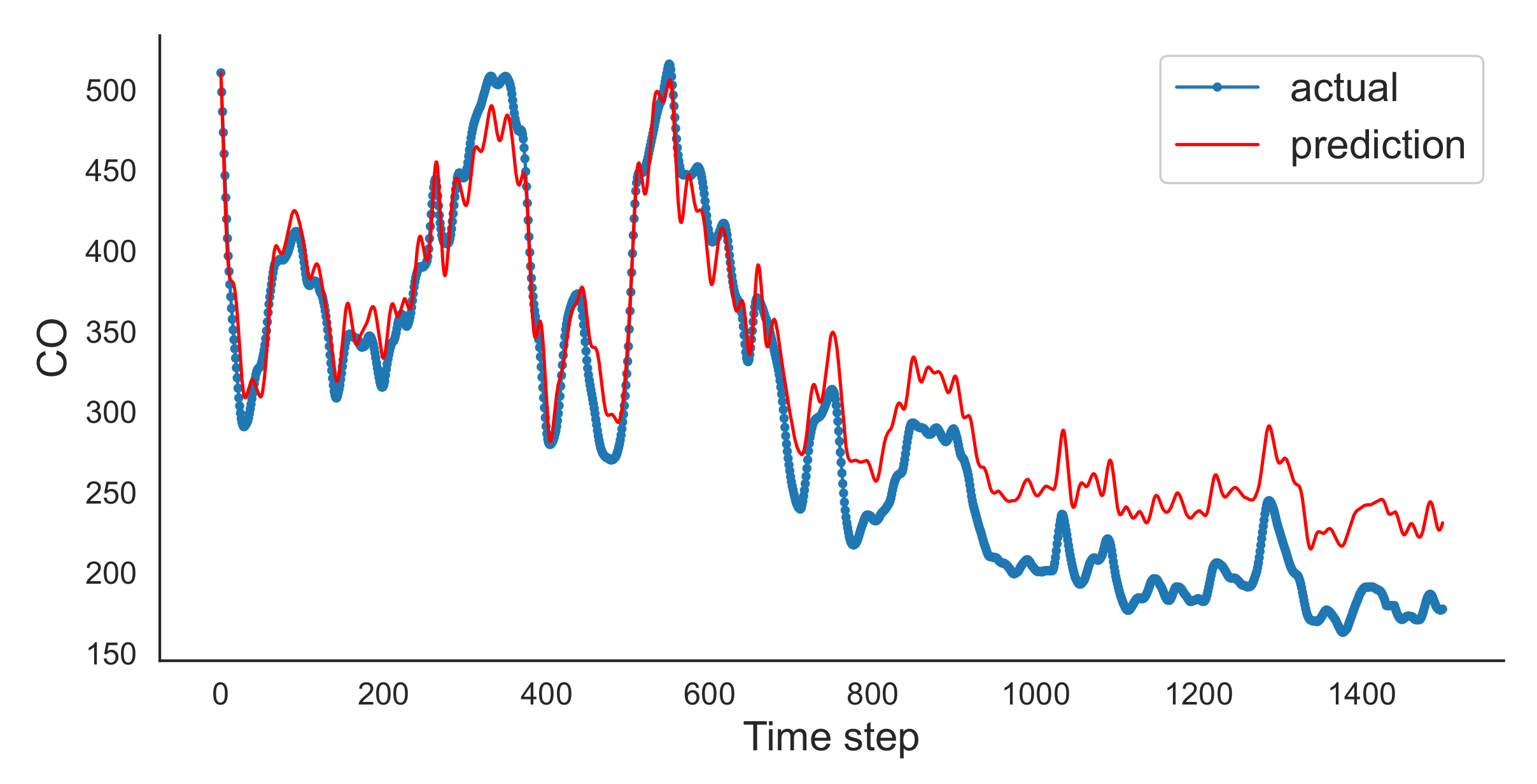
We run the univariate LSTM for three batch numbers, namely 100, 1000, and 7000. We trained the LSTM in 100 epochs. We noticed that when the batch number is equal to 100 and 1000, there is a deviation from the actual values as can be observed in
Figure 7 and
Figure 8. In
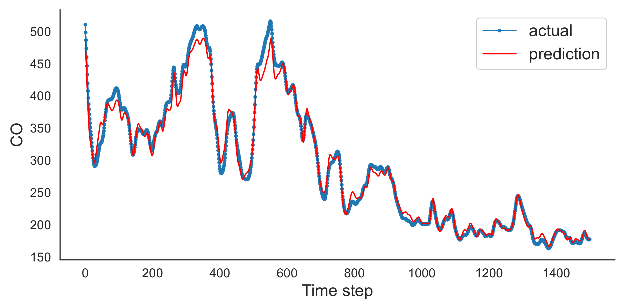
Figure 9, with the batch number equal to 7000, the reader can see that the prediction values are very close to the actual values. This may be an indication of a better generalisation, a sweet spot for the entire dataset. The results from the 100 and 1000 values batch, show the results that are poorer; thus we may convey that we do not have an adequate generalisation.
Figure 10,
Figure 11 and
Figure 12 illustrate the train and test loss for the three cases. An it can be observed, the larger the batch number the smoother the curves and the smaller the loss numbers, as seen in
Figure 10,
Figure 11 and
Figure 12.
Moreover, we provide the RMSE and MAE for the train and test of the three cases as they can be seen in
Table 2. We can see that train RMSE for the batch equal to 100 is significantly high as opposed to the batch number 1000 and 7000. On the other hand, the train MAE, test MAE, and test RMSE are higher with the batch number equal to 1000 than the batch number equal to 100. The best numbers are accomplished with the batch size equal to 7000. The results shown in the
Table 2 show that the experiments with the batch number equal to 7000 exhibit better accuracy than the experiments with the 100 and 1000 values, and the deviation from the actual values. Hence, we see that these interpretations are better when using the 7000 values batch. The RMSE also needs to be less than the MAE by definition, which is also the case in our experiments. This is because the errors are squared before they are averaged, the RMSE gives a relatively high weight to large errors. This means the RMSE is most useful when large errors are particularly undesirable.
Thereafter we compared the LSTM approach with the well-known ARIMA model. An ARIMA (1,1,0) model if fitted. This sets the lag value to 1 for autoregression and to speed up the prediction, uses a difference order of 1 to make the time series stationary, and uses a moving average model of 0. The forecast function is encapsulated, which performs a one-step forecast by using the model. We split the dataset to a train and test dataset with 80% and 20% data points respectively. The train set was used to fit the model and generate a prediction for every element on the test part of the dataset. For the ARIMA rolling forecast, we manually inspect all observations in a list, namely history, which is fed with the training data and to which new observations are appended for each iteration. The results of the comparison between the LSTM and the ARIMA is shown in
Figure 13. Here, it can be seen that the ARIMA model predictions are very close to the actual values. However, the LSTM does not perform very badly, being close to the actual values as well. For this problem, the ARIMA model seems to be better; however, in future work, the two models will be evaluated to multivariate problems.
The ARIMA model [
26] works quite well with the PM concentrations and the predicted values are close to the actual values, which verifies our results. Moreover, the LSTM, in this work [
24], works quite well in predicting the value that is under investigation. The reader can check the value error percentage, which is indeed quite good. This also verifies the results of our paper because the LSTM does perform significantly well when predicting the CO values.
7. Conclusions
In this paper, we addressed the issue of air quality in the broader area of the port of Igoumenitsa in Greece. Many studies have been done for environmental monitoring [
38] especially for coastal areas and [
39] and many approaches have been proposed to provide environmental risk management in seaports [
40] because they are areas of particular interest. We use the data gathered at a wireless environmental sensors system, which is installed in the Port of Igoumenitsa, Greece. Here, we selected the CO measurements to perform a prediction by using a machine-learning model. Specifically, we used a univariate LSTM, to predict future values with respect to the actual ones. Our work comprised the use of the univariate LSTM with different batch numbers, namely 100, 1000, and 7000. We showed that batch number 7000 exhibited the best results of RMSE and MAE, concerning the train and test loss. Moreover, the prediction was much closer than the other two cases. Furthermore, we compared the LSTM with the ARIMA model and showed that the ARIMA exhibited better prediction while the LSTM performed quite well as well.
For future work, we aim to use a bidirectional LSTM for comparison and a multivariate approach, to include a number of the other environmental parameters available from the environmental wireless station. Furthermore, because we maintain another station proximate to the premises of the university branch, which resides a few kilometers from the port, we aim to compare the readings from the two stations to visually perceive patterns. Lastly, our objective is to coalesce the two stations into a multivariate model. Moreover, we will use the dataset without the smoothing procedure, to indicate potential drawbacks in the prediction. We aim to encapsulate the works in [
41,
42] to platforms of limited resources.


