Curvature Correction for Crack Depth Measurement Using Ultrasonic Pulse Velocity

Abstract

This study investigates the application of Ultrasonic Pulse Velocity (UPV) for crack depth estimation in cylindrical structures, focusing on two approaches: reference measurement and dual measurement. It addresses the challenge of applying UPV to curved surfaces, a scenario less studied than that of flat surfaces. The paper details the modification of UPV methodologies to account for curvature, presenting analytic solutions and numerical validations for both approaches. The findings reveal that curvature-adjusted equations yield accurate crack depth estimations, enhancing the reliability of UPV in diverse structural contexts. The study contributes to safer and more effective structural health monitoring, particularly in cylindrical infrastructures like columns and foundations.

1. Introduction

Concrete cracks. Despite extensive research and efforts by scientists, researchers, and engineers, it remains a persistent challenge in the field of civil engineering. Cracks in concrete occur due to a multitude of factors, including plastic [1,2], freeze/thaw cycles [3,4], improper curing and drying [5,6], overloading, premature loading (before 28 days of curing), improper mix design, and thermal cracking [7,8,9], etc. Not all concrete cracks pose structural concerns; some may not necessitate immediate intervention [10,11]. However, in some other cases, cracks demand imminent repair or even complete replacement of the concrete structure. Ignoring these signs can lead to a cascade of problems, including but not limited to structural failure [12,13], potential safety hazards, corrosion of the embedded steel reinforcement [14,15,16], a decline in aesthetic appeal, diminished property value, and increasing costs for eventual repairs.

The problem of cracking extends beyond concrete to structures made of stone materials such as granite [17,18,19,20], marble [21,22,23], and sandstone. These materials, often more costly than concrete, are sometimes used in historic buildings, adding an extra layer of complexity to their maintenance and preservation. Cracks in such structures not only pose a risk to their structural integrity but also bear cultural and historical significance, making their preservation a matter of utmost importance.

The depth and nature of cracks in both concrete and stone materials play a crucial role in determining the appropriate course of action. Minor, surface-level cracks may require simple cosmetic fixes, whereas deeper, structural cracks might call for more extensive repair techniques. In the case of historical structures, the preservation approach needs to be carefully selected to maintain the building’s integrity and historical value.

The most direct method for assessing the depth of a crack is through core sampling; this approach typically involves extracting cores and subsequently visually examining the corehole and the core to identify the depth of the crack [24]. However, this method is destructive to the structure. For Non-Destructive Evaluation (NDE) of concrete and stone structures [25,26,27], some NDE methods may not be suitable. For example, Eddy Current Testing, primarily used for detecting surface and near-surface defects, may have limited applicability due to the non-conductive nature of these materials. Infrared thermography, which identifies temperature variations on a structure’s surface, indicating potential issues like cracks or voids, is a quick and non-contact method. However, its effectiveness hinges on specific environmental conditions. X-ray radiography, while offering detailed internal imaging, requires access to both sides of the structure, which may not always be feasible. Additionally, the use of X-rays raises safety concerns and demands specialized equipment and trained professionals. Interpreting X-ray images also requires a high level of expertise.

In contrast, the Ultrasonic Pulse Velocity (UPV) test presents an effective non-destructive alternative for estimating the depth of cracks. The UPV-based methodology entails generating high-frequency ultrasonic pulses, which are transmitted into the material. The time of flight (TOF) of these pulses, namely the duration they travel within the material from the transmitter to the receiver, is measured. In an intact structure, the first pulse to reach the receiver follows the shortest path—a straight line between the transmitter and receiver on the structural surface. In the presence of a crack, this path is obstructed, causing the pulses to take a transmitter-crack tip-receiver path due to diffraction. Consequently, by analyzing the TOF of the first arriving pulse, the depth of the crack can be estimated [28].

Numerous examples exist demonstrating the application of UPV and TOF-based NDT approaches for estimating crack depth [29,30,31,32,33]. Predominantly, UPV is employed to measure cracks on flat surfaces in concrete structures. However, when dealing with structures possessing cylindrical geometries, such as columns or pole foundations, the surface curvature must be taken into account. This paper addresses the impact of curvature on UPV measurements and discusses necessary corrections. Two distinct methodologies of UPV crack measurement are explored: the reference measurement approach and the dual measurement approach. Analytic solutions and numerical validations are provided for both approaches in this study, enhancing the reliability of the methods. This advancement ultimately contributes to the improved safety and longevity of infrastructural assets.

2. Estimation of Crack Depth via UPV with Reference Ultrasonic Velocity

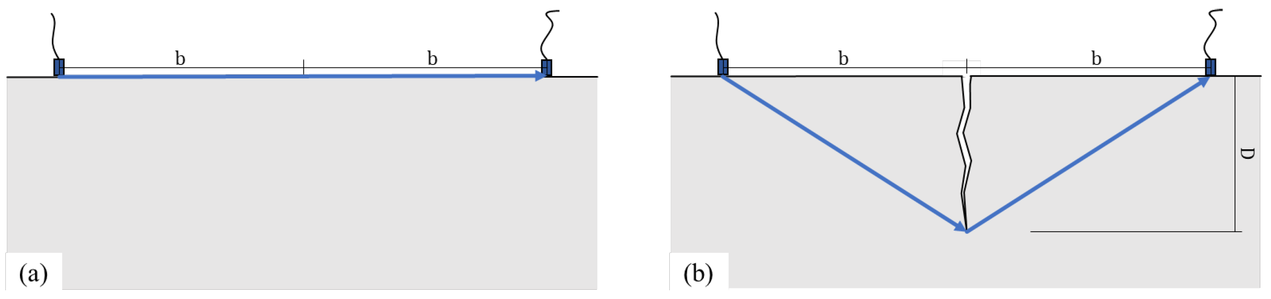
2.1. Principle of Reference Measurement Approach

Assuming a constant sound velocity along different paths within the test material, the depth of the crack can be estimated by comparing the TOF of a reference measurement with measurements taken when the transducers are placed equidistantly from the crack at certain distances, b [28]. The reference measurement serves to determine the ultrasonic velocity of the material. This velocity can be straightforwardly calculated by dividing the distance between the transducers, $2b$, by the TOF of the pulse traveling along the surface, $T_s$, shown as Figure 1:

$$c=2·b/T_s$$

(1)

The depth of the crack, D, can thereby be calculated by the velocity of ultrasound, c, and the TOF that measured from the cracked surface, $T_c$,

$$D=\sqrt{{(c·T_c/2)}^2-b^2}$$

(2)

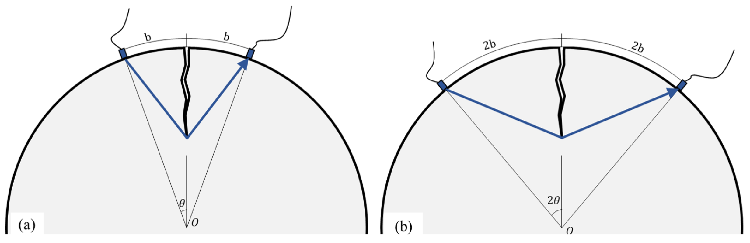
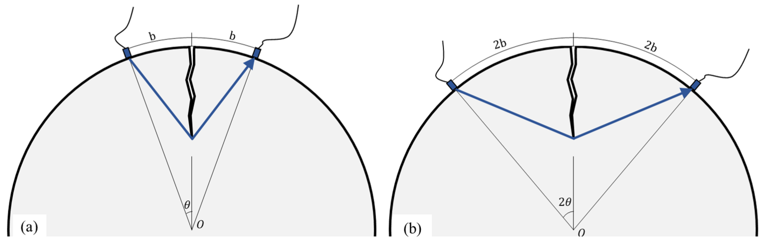
2.2. Curvature Correction of Reference Measurement Approach

For cylindrical structure, the surface curvature, denoted as $1/R$ where R is the column radius, influences crack measurements. Contrasting with flat surfaces, the shortest ultrasonic path between transducers in the structure is not along the surface, but a straight line through its interior, as illustrated in Figure 2. This deviation in path necessitates a recalculation of the ultrasonic velocity c, which can be achieved using the following Equation (3):

$$c=\frac{2R·sin\theta }{T_0^{\prime }},$$

(3)

where $T_0^{\prime }$ is the reference TOF for cylindrical structure and

$$\theta =b/R$$

(4)

The revised crack depth is determined using Equation (5),

$$D^{\prime }=D_1+D_2,$$

(5)

where $D_1$ represents the minimal detectable crack depth. If a crack is shallower than $D_1$, the pulse travels directly from transmitter to receiver without interacting with the crack, as per Equation (6),

$$D_1=R(1-cos\theta ).$$

(6)

The depth $D_2$ is calculated using Equation (7).

$$D_2=\sqrt{{(c·T_c^{\prime }/2)}^2-{(Rsin\theta )}^2}$$

(7)

Given the prevalence of UPV devices on the market that are predominantly designed to measure crack depth on flat surfaces and often feature an automated depth display, it is beneficial to formulate a relationship between the depth, $D^{\prime }$, as measured on a curved surface, and the automated depth, D, that these devices typically calculate for flat surfaces. Equations (4) and (5) can be rewrittten as Equation (8) and Equation (9), respectively.

$$\sqrt{{(\frac{T_c}{T_s})}^2-1}=\frac{D}{b}$$

(8)

$$\sqrt{{(\frac{T_c^{\prime }}{T_s^{\prime }})}^2-1}=\frac{D^{\prime }-R(1-cos\theta )}{Rsin\theta }$$

(9)

By virtue of Equations (8) and (9), the relation of the actual crack depth, $D^{\prime }$, and the depth that automated measured using the devices that are designated for flat surface, D, can be expressed as

$$\frac{D}{b}=\frac{D^{\prime }-R(1-cos\theta )}{Rsin\theta }$$

(10)

According to Equation (10), the measured depth is linearly dependent on the actual depth. When measuring a surface with very small curvature, the difference between these values should be negligible. In such cases, $R>>b$, the approximation $1-cos\theta \approx 0$ and $sin\theta \approx b/R$ can be applied due to the minimal curvature effect. Consequently, under these conditions, the adjusted depth $D^{\prime }$ is approximately equal to the automated depth measurement, D. Figure 3 presents an engineering chart designed for quick depth correction. This chart is particularly useful for interpreting measurements obtained from devices originally designed for flat surfaces, enabling their effective application on surfaces with curvature.

The method incorporates a reference measurement that offers significant efficiency, allowing for the measurement of multiple crack depths with a single reference measurement. This approach, however, operates under the assumption that the speed of sound remains consistent throughout the material, an assumption that may not always hold true in field applications [34]. To address this potential discrepancy, the use of UPV with dual measurements can be employed.

3. Estimation of Crack Depth via UPV with Dual Measurement

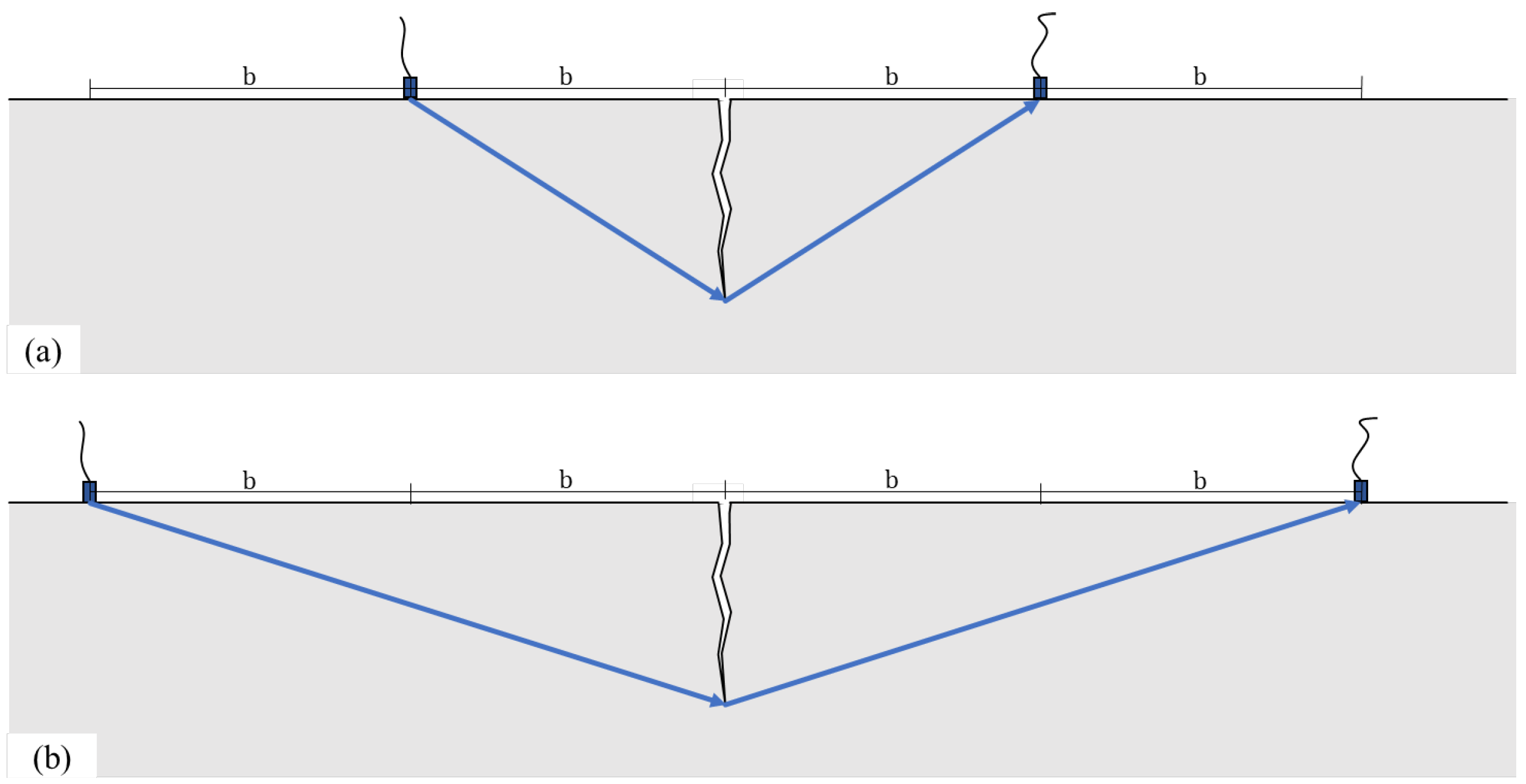
3.1. Principle of Dual Measurement Approach

The UPV method with dual measurements is not affected by differences in the speed of sound across different areas of the structure because it compares the TOF of two measurements conducted in the same area. In this method, the first and second measurements position the transducers at distances of b and $2b$ from the crack, respectively, as shown in Figure 4. Such an approach ensures that the speed of sound within different regions of the structure do not impact the accuracy of the crack depth measurement, as both measurements are taken under same location.

In this arrangement, the depth of the crack can be calculated using the following equation [28]:

$$D=b\sqrt{\frac{4T_1^2-T_2^2}{T_2^2-T_1^2}},$$

(11)

where $T_1$ and $T_2$ represent the TOF measured when the distance between the transducers is equal to b and $2b$, respectively.

3.2. Curvature Correction of Dual Measurement Approach

Using UPV with dual measurements requires that the depth of the crack be greater than $R·(1-cos2\theta )$. As shown in Figure 5, when the distance between the transducers and the crack on the surface is b, the half-length of the ultrasonic pulse’s travel path is governed by the Pythagorean theorem, yielding the following equation:

$${(T_1^{\prime }·c/2)}^2={(R·sin\theta )}^2+{(D^{\prime }-R(1-cos\theta ))}^2,$$

(12)

likewise, when the distance between the transducers and the crack is $2b$, the half-length of the ultrasonic pulse’s travel path can be described by:

$${(T_2^{\prime }·c/2)}^2={(R·sin2\theta )}^2+{(D^{\prime }-R(1-cos2\theta ))}^2.$$

(13)

Utilizing Equations (12) and (13), the depth of a crack in a cylindrical structure, $D^{\prime }$, can be determined by the ratio of the TOF measured at different transducer-to-crack surface distances. These measurements are conducted with the transducer–crack surface distance set at b and $2b$, represented as $T_1^{\prime }$ and $T_2^{\prime }$, respectively.

$${(\frac{T_1^{\prime }}{T_2^{\prime }})}^2=\frac{{(R·sin\theta )}^2+{(D^{\prime }-R(1-cos\theta ))}^2}{{(R·sin2\theta )}^2+{(D^{\prime }-R(1-cos2\theta ))}^2}.$$

(14)

The speed of sound, c, is eliminated from the equations in this methodology, implying that the method should not be impacted by variations in the speed of sound within different areas of the materials. Rearranging Equation (11), one has

$${(\frac{T_1}{T_2})}^2=\frac{D^2+b^2}{D^2+4b^2}.$$

(15)

By virtue of Equations (14) and (15), one has

$$\frac{D^2+b^2}{D^2+4b^2}=\frac{{(R·sin\theta )}^2+{(D^{\prime }-R(1-cos\theta ))}^2}{{(R·sin2\theta )}^2+{(D^{\prime }-R(1-cos2\theta ))}^2}.$$

(16)

To verify the equation, when the curvature is negligible ($R>>b$), and the automated measurement of depth, D, is expected to be close to the actual crack depth, $D^{\prime }$, the simplification including $R·sin\theta =b$, $R·sin2\theta =2b$, $1-cos\theta =0$, can be applied. In this scenario, the left-hand side and right-hand side of the equation will take a similar form. Given the automation of crack depth measurement and the complexity inherent in the analytical expression of $D^{\prime }$, an engineering chart has been provided, Figure 6.

4. Numerical Simulation

In evaluating structural integrity, the spectral finite element method (FEM) is recognized as a more effective technique for crack analysis [35]. Nevertheless, in our investigation, we utilized COMSOL Multiphysics^® software for numerical verification, specifically selecting the “Elastic Waves, Time Explicit” physics interface to model wave propagation. This interface adeptly manages the linear elastic wave equation in its velocity–strain formulation. The execution of this modeling utilizes the discontinuous Galerkin finite element method (dG-FEM), which is integrated with an explicit time integration scheme [36,37]. Such a methodological approach allows for a detailed and precise simulation of wave propagation dynamics. The outcomes of this simulation offer a clear and intuitive visualization of the path traversed by the wave and how it interacts with the crack, thus providing valuable insights into wave behavior in the flat and curved structure tested by different configurations.

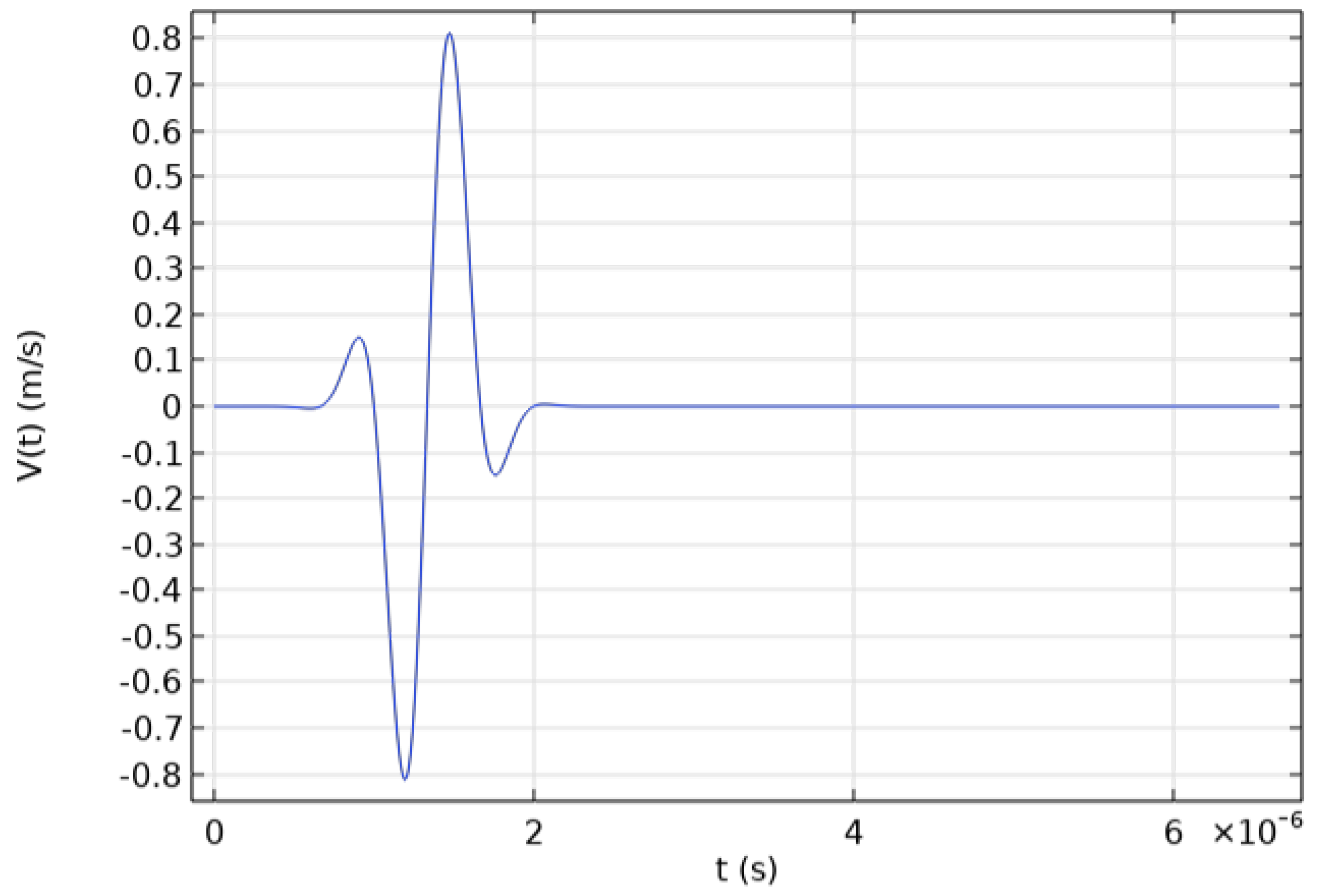
4.1. Model Parameters

Seven models with diffract geometries were built for the finite element analysis. Three of these models were specifically crafted to simulate UPV measurements on flat surfaces, as illustrated in Figure 7. The other four models were used to replicate UPV measurements on curved surfaces, as depicted in Figure 8.

In these simulations, transducers are represented as round notches. The surface distance between the transducers is standardized at 20 cm for models (a), (b), (i), (ii), and (iii). For models (c) and (iv), this distance is extended to 40 cm. The crack depth also varies among the models: it is set at 4 cm for models (b) and (c), 20 cm for models (ii) and (iv), and 2.6 cm for model (iii). The samples in models (a), (b), and (c) have a height of 20 cm, while the models designed for curved surfaces (i), (ii), (iii), and (iv) feature a radius of curvature of 30 cm.

These models enable the simulation of different UPV measurement configurations. For flat surfaces, models (a) and (b) (enclosed within a solid box in Figure 7) simulate UPV with reference measurement. Correspondingly, for curved surfaces, models (i) and (ii) (also within a solid box in Figure 8) are used for the same purpose. In addition, UPV with multiple measurements is represented by models (b) and (c) for flat surfaces (delineated by a dashed box in Figure 7) and by models (ii) and (iv) for curved surfaces (indicated by a dashed-dotted box in Figure 8). This array of configurations facilitates a comprehensive study of UPV methodologies across different geometric scenarios, thereby enriching the understanding of the impact of surface curvature and measurement techniques on ultrasonic wave propagation and crack detection.

The material selected to represent the structure was a built-in material option for concrete, characterized by a density of 2300 kg/m², Young’s modulus of 25 GPa, and a Poisson’s ratio of 0.2. Given these material properties, the velocity of acoustic waves in the simulations was determined: 3475 m/s for compressive (P-) waves and 2128 m/s for shear (S-) waves. Low-reflect boundary conditions were applied to the bottom boundary of each model. This implementation was crucial for achieving a clearer observation of the propagation of the first pulse that arrives at the receiver. The pulse used in these simulations was formulated as the product of a Gaussian function and a sine function, as described in Equation (17) and shown in Figure 9. The frequency of this pulse was set to 1.5 MHz. Noting that for UPV application in concrete, the typical pulse frequency ranges into the thousands of Hz. Should the frequency reach MHz levels, it leads to rapid attenuation, diminishing the detection range. The decision to use a frequency of 1.5 MHz in this numerical simulations was primarily motivated by computational efficiency. Employing a higher frequency enables modeling the system on a significantly smaller scale than would not be possible with kHz frequencies, thereby saving computational resources. Furthermore, choosing not to apply attenuation in the simulation was intended to enhance the visibility of the acoustic pulse progression. The maximum mesh size was limited to two-thirds of the wavelength of the ultrasonic pulse and time step for the simulations was set to 0.03 ms.

$$V\left(t\right)=exp(-{(2t{f}_0-4)}^2)·sin\left(2\pi f_{0}t\right)$$

(17)

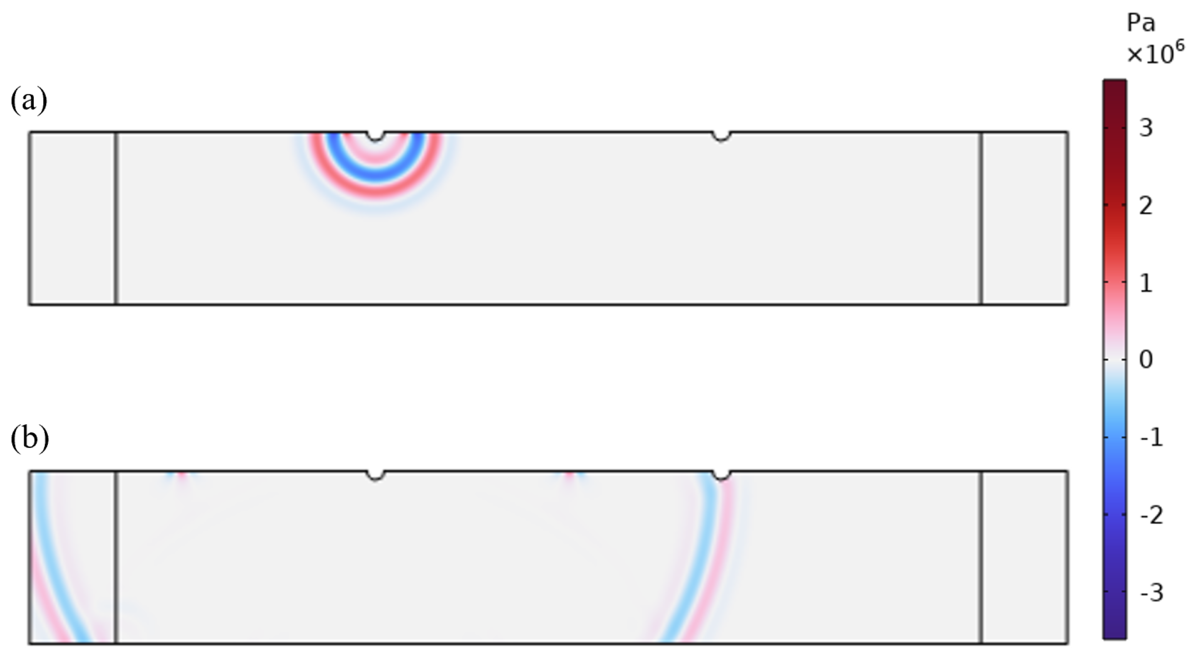
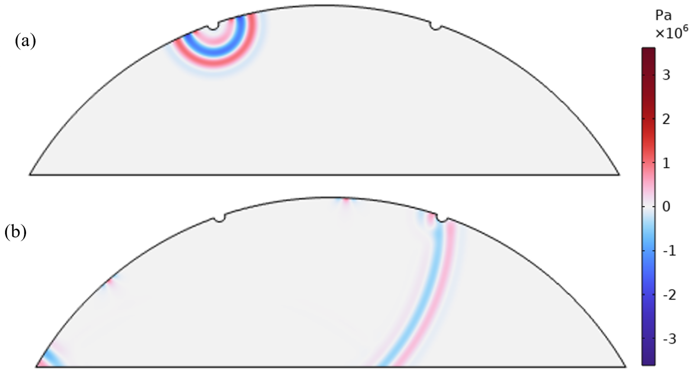
4.2. Results for Flat Surfaces

The acoustic pulse propagation simulation in a concrete with transducers positioned on a flat surface, separated by a distance of $2b$, is illustrated in two distinct scenarios: without a crack, Figure 10, and with a crack present, Figure 11.

Configuration 1 (Figure 7, Solid Box): In the scenario depicted in Figure 12a, where no crack was present, the pulse TOF was measured at 0.567 ms, leading to a calculated sound speed of 3527 m/s. Conversely, in the scenario with a crack, as illustrated in Figure 12b, the pulse TOF increased to 0.611 ms. Substituting this value into Figure 2 allowed for the determination of the crack depth, calculated to be 4.03 cm.

Configuration 2 (Figure 7, Dashed Box): When the surface distance between the transducers was set to $2b$, the TOF was recorded as 1.157 ms, Figure 13b. By substituting these values into Figure 11, the calculated depth of the crack was determined to be 4 cm.

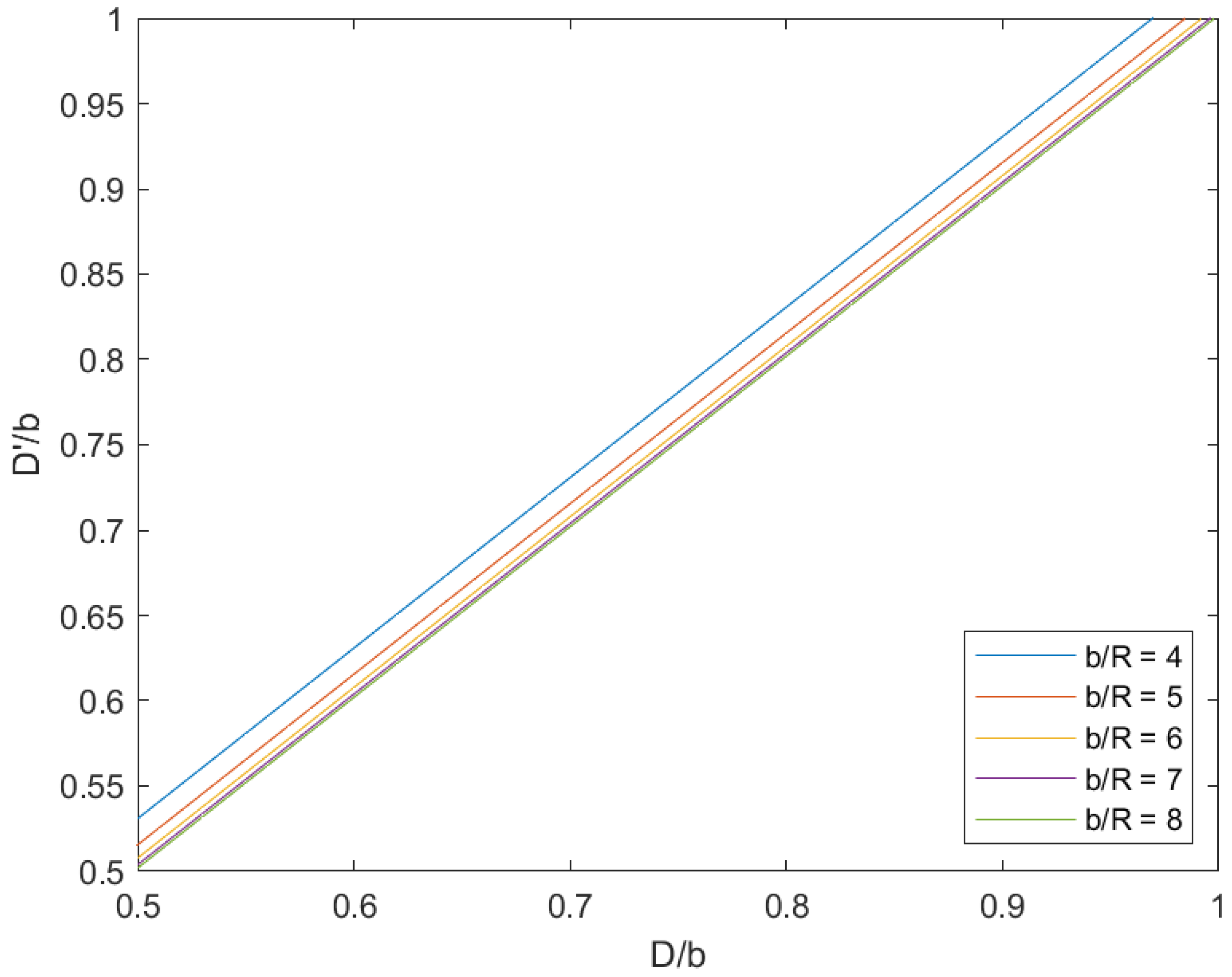
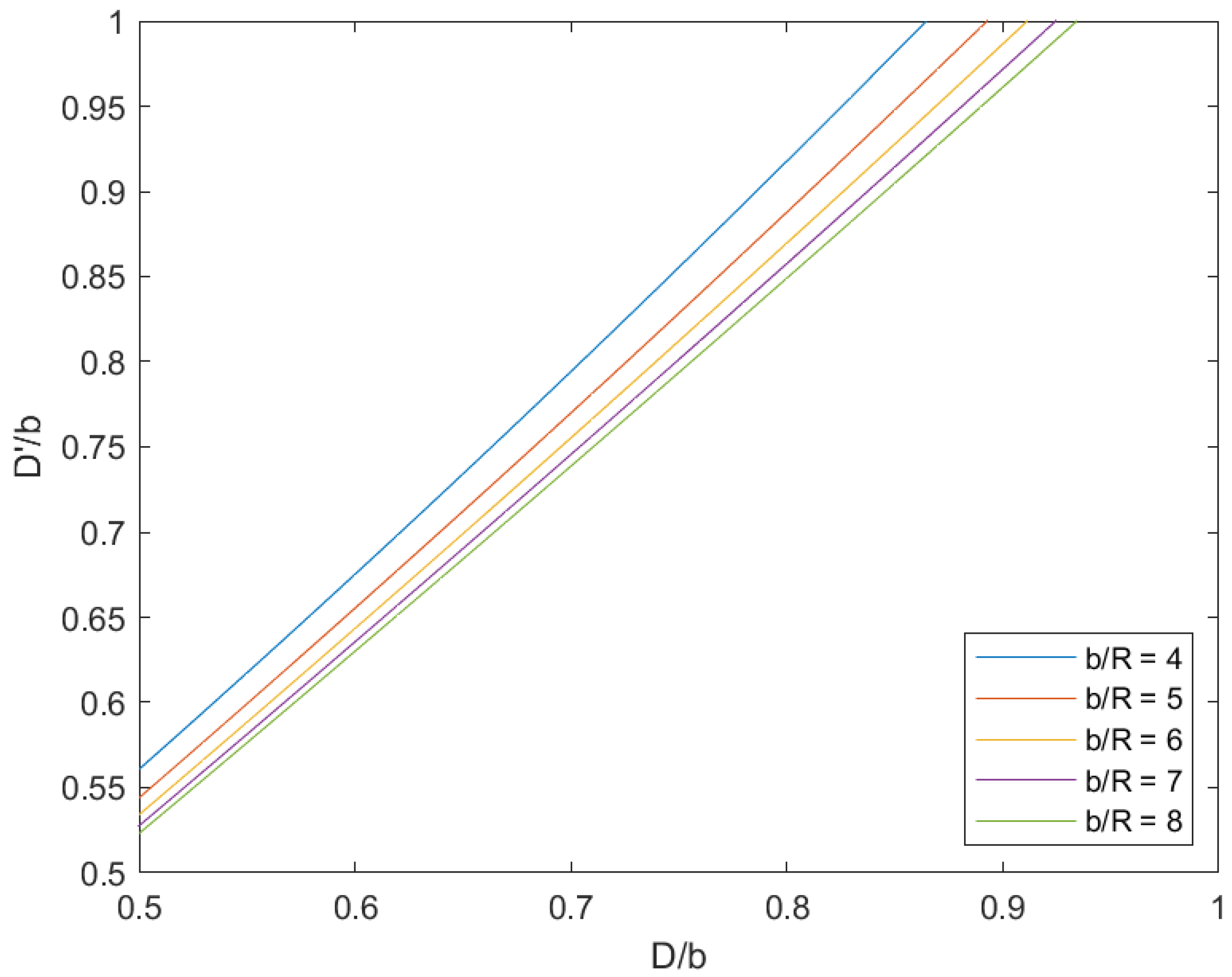
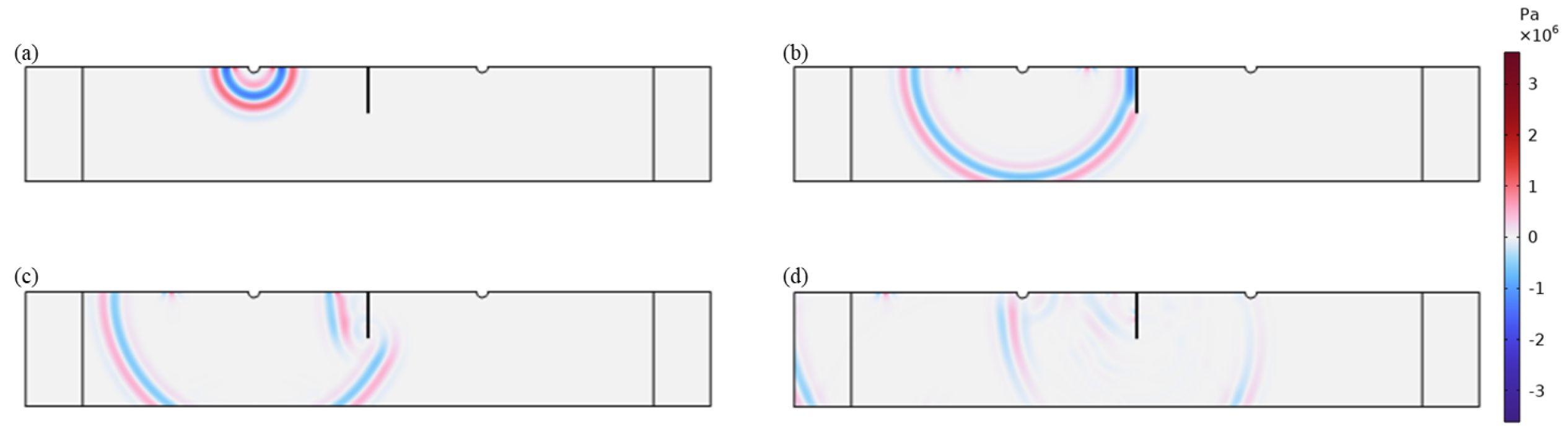
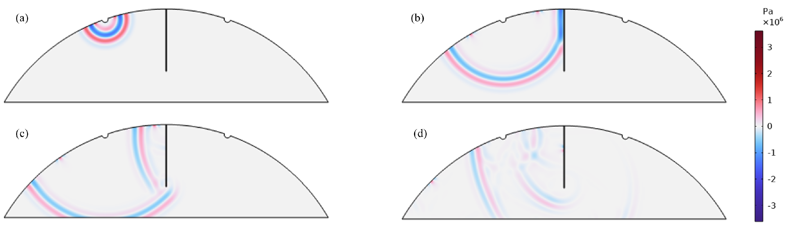
4.3. Results for Curved Surfaces

The simulated propagation of an acoustic pulse in concrete, with transducers situated on a surface with curvature and spaced $2b$ apart, was demonstrated under two conditions: absence of a crack, as indicated in Figure 14, and presence of a crack, as represented in Figure 15.

Configuration 3 (Figure 8, Solid Box): As depicted in Figure 16a, when transducers were placed on a curved surface with a surface-measured distance of $2b$ between them, the TOF was 0.553 ms. Applying this value to Equation (3), the speed of sound was calculated as 3500 m/s. In the presence of a crack, Figure 16b, the TOF increased to 0.733 ms. Substituting these values into Equation (9), the depth of the crack was calculated to be 4 cm.

Configuration 4 (Figure 8, Dotted Box): In cases where the crack depth was too shallow, the TOF of the pulse in the structure was identical to that of an intact one. This is demonstrated in Figure 17, where the TOF of the pulse is 0.553 ms, which is the same as the TOF in the intact structure.

Configuration 5 (Figure 8, Dashed Box): Figure 18b shows the TOF measured from a curved surface, where the distance between the transducers, measured from the surface, is $2b$. By substituting the TOF value into the Equation (14), the depth of the crack was calculated as 4.2 cm.

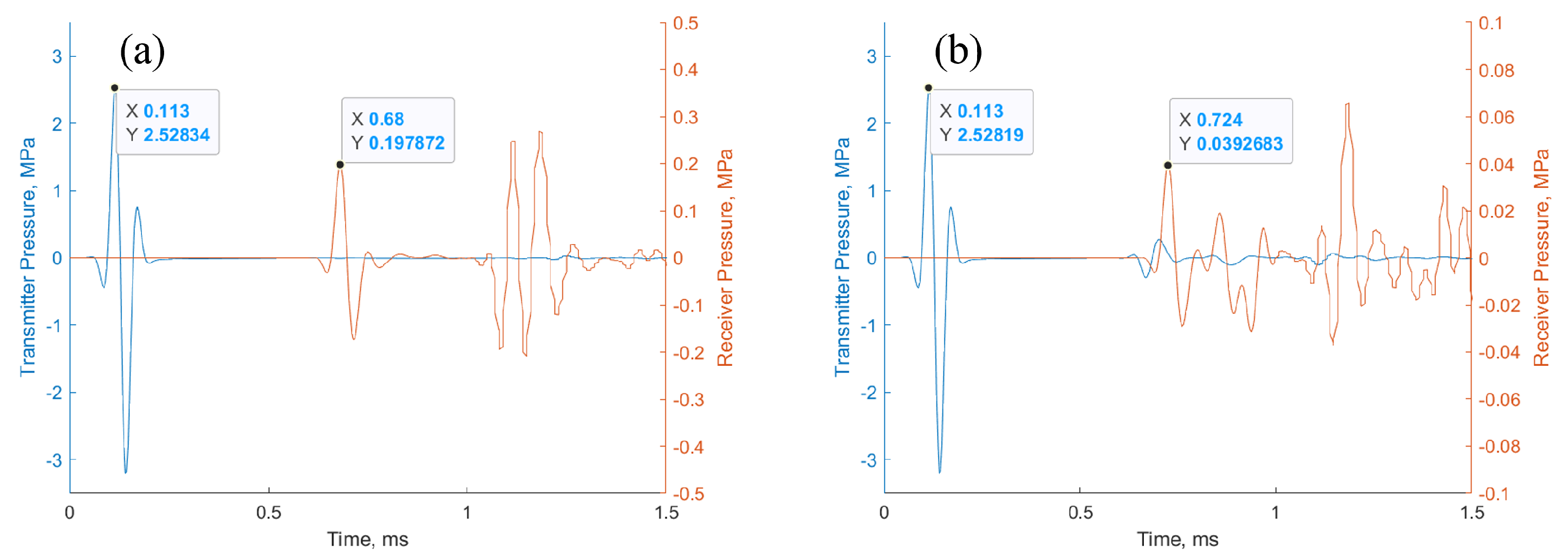
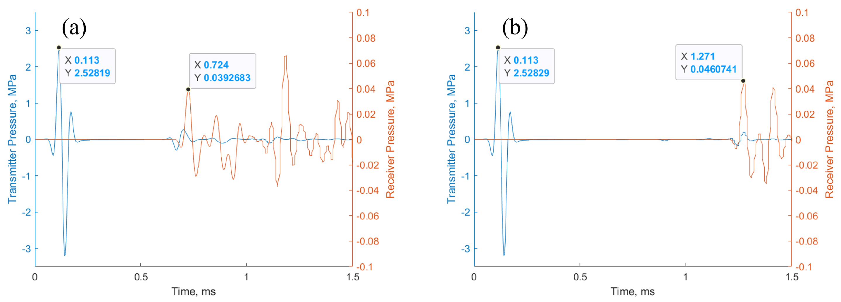
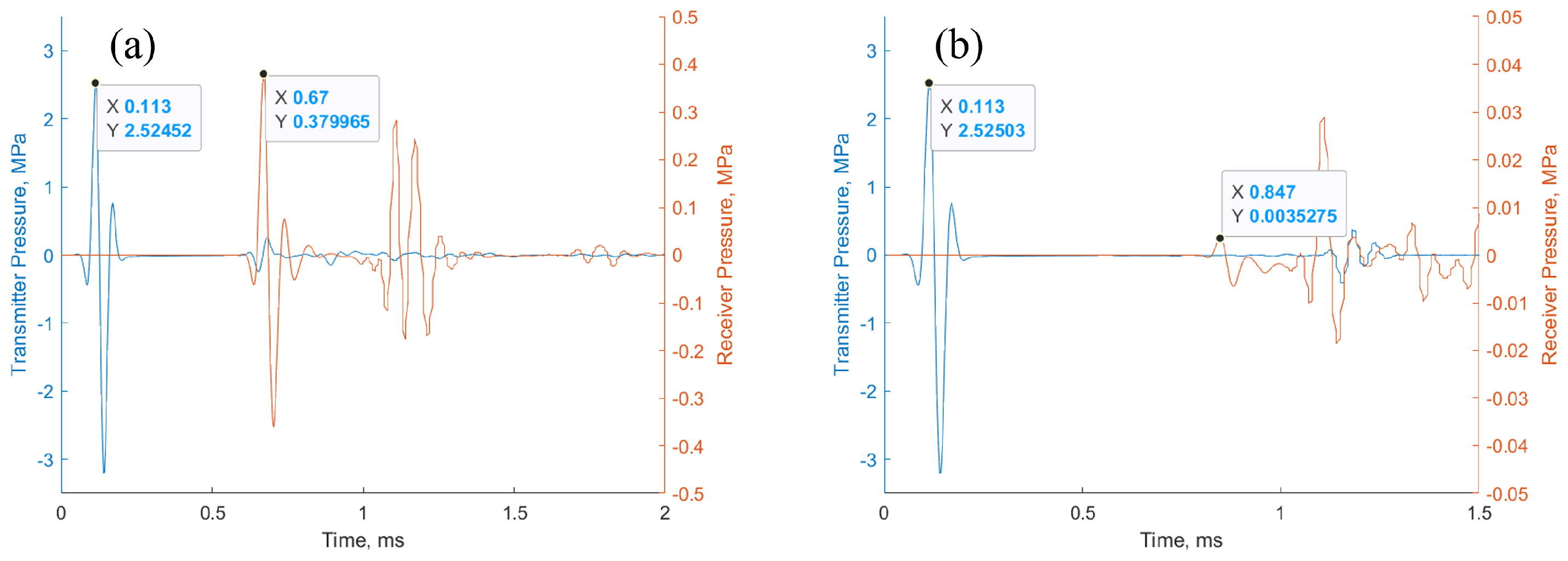
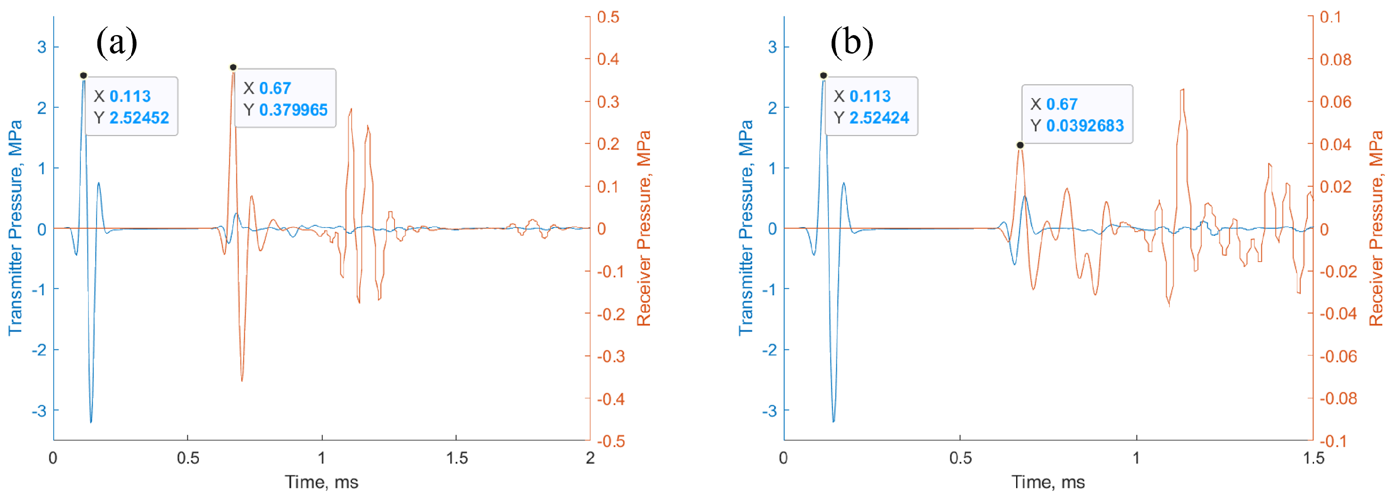
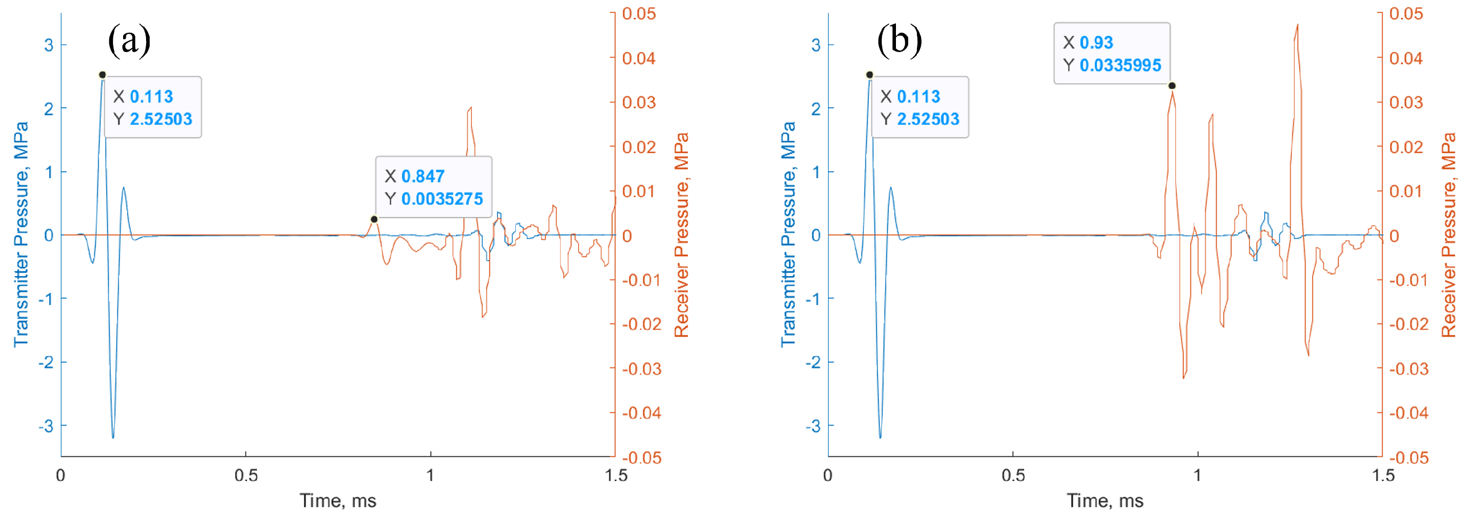
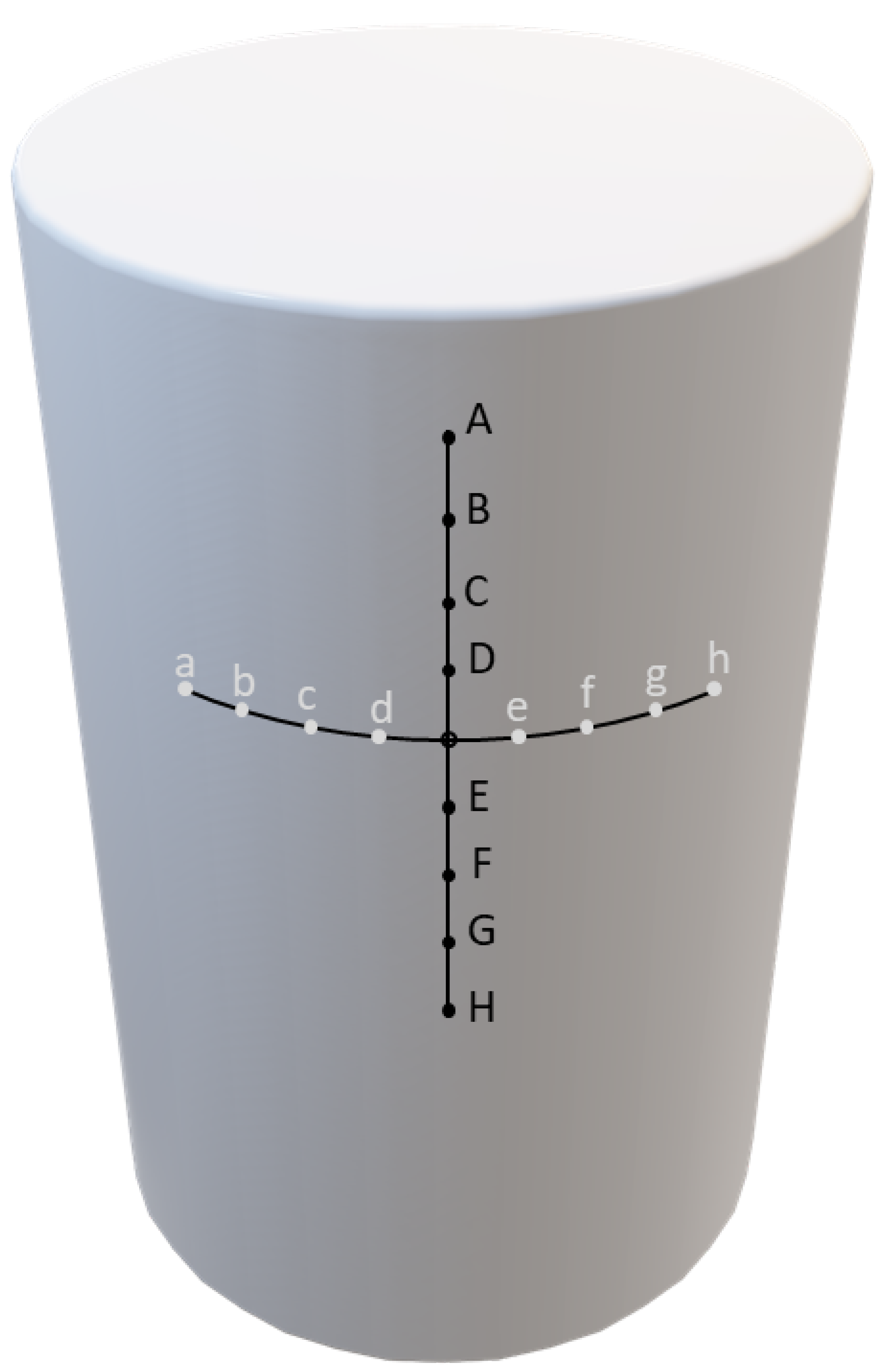
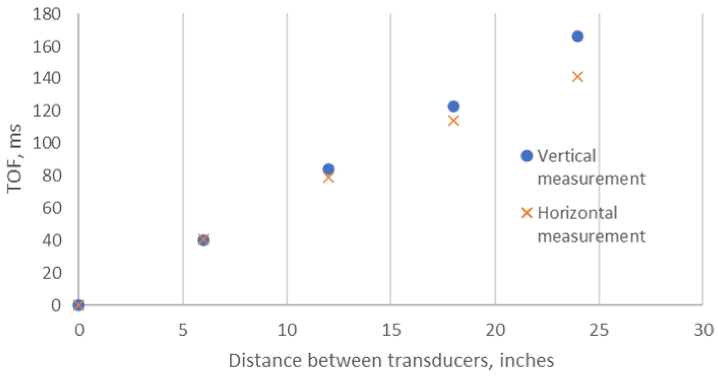
5. Experimental Verification

This study is based on an assumption: the first ultrasonic pulse received by the receiver travels via the interior of the column instead of its surface. To verify this assumption, an experiment was designed. The device used for conducting the UPV test is the PUNDIT PL-200, made by Proceq®. The ultrasonic pulses were generated and received by a transducer with a designated frequency of 54 kHz (part number 325 40 177-B). The test object is a marble column with a diameter of 2 feet (60.96 cm). As shown in Figure 19, 16 points were selected as the transducer locations. These points form crosses, with eight points (gray points) aligned horizontally and eight points (black points) aligned vertically. The distance measured from the surface between each adherent point is 3 inches (7.62 cm). In total, there were eight UPV tests conducted: four measured vertically and four measured horizontally. For each measurement, the two transducers were placed at points located on the same line (vertical/horizontal) and had an equal surface distance from the central points of the cross. Hence, for the vertical measurements, the placement of the transducers was at points D–E, C–F, B–G, and A–H, with the respective distances between them being 6 inches (15.24 cm), 12 inches (30.48 cm), 18 inches (45.72 cm), and 24 inches (60.96 cm). In the case of horizontal measurements, the transducers were positioned at points d-e, c-f, b-g, and a-h, also with corresponding distances of 6 inches (15.24 cm), 12 inches (30.48 cm), 18 inches (45.72 cm), and 24 inches (60.96 cm) between them.

The sound speed of these measurements should be considered constant since the transducers were placed in a nearby area of a same material. In this configuration, the vertical measurements shall be considered as flat surface measurements since the vertical surface of a column is flat. The TOF for the vertical measurement should be linearly dependent on the distance between the transducers. The horizontal UPV measurement, in contrast, will be affected by the curvature. The TOF for the horizontal measurement should be less than the TOF for the vertical measurement with the same surface distance because the ultrasonic pulse travels a shorter distance within the interior of the column compared to the surface. The test results are shown in Figure 20.

Indeed, as the results show, the TOF and distance between the transducers have a linear relationship for the vertical measurements. For the horizontal measurements, the greater the distance between the transducers, the greater the deviation between the TOF measured vertically and horizontally, as expected. This result confirms that ultrasonic pulses travel through the interior of the column and that correction of the measurement will be needed when the curvature effect cannot be ignored.

6. Discussion

This study explores the application of UPV for estimating crack depth in cylindrical structures. It examines two UPV approaches: the reference measurement approach and the dual measurement approach. As elucidated in Section 2 and Section 3, the path of acoustic pulse propagation in cylindrical structures differs from that in flat-surfaced structures. Consequently, UPV results obtained from flat and curved surfaces require distinct interpretation methods. The study presents specific equations for UPV with curvature adjustments for accurate crack depth estimation.

Subsequently, numerical simulations were performed to validate these equations. By substituting the simulated TOF values into the derived equations, the calculated values for the speed of sound and crack depth closely matched the input values, exhibiting minimal error. This accuracy suggests the validity of the proposed equations. An experiment was conducted to verify the hypothesis that ultrasonic pulses within a curved surface travel through its interior rather than along its surface. Conducted on a marble column with a 2-foot diameter, twelve transducer locations were selected, forming crosses with six points, each aligned horizontally and vertically. The experiment included six UPV tests, divided equally between vertical and horizontal measurements. Vertical tests were considered to be flat surface measurements, with the TOF expected to linearly correlate with the distance between transducers. In contrast, horizontal tests showed deviations due to curvature, suggesting that pulses travel shorter internal paths, thereby highlighting the need for measurement adjustments in structures with curvature.

Furthermore, the study proposes the use of engineer charts for estimating crack depth in cylindrical structures. These charts aid in adjusting the automated crack depth calculations designed for flat surface UPV measurements. The experimental outcomes reveal that a reduction in curvature correlates with diminished variance between the measured depth and the depth determined by automation for both reference and dual measurement methods. The reference measurement method consistently shows less error compared to the dual measurement method. Given considerations of both accuracy and operational efficiency, the reference measurement technique is recommended for evaluating crack depth within cylindrical infrastructures, assuming it meets the field conditions’ requirements.

In summary, this research emphasizes the need for geometry-specific UPV methods for accurate crack detection in cylindrical structures. It introduces curvature-adjusted equations, validated by simulations, to improve accuracy in such scenarios. The study recommends the reference measurement approach for its lower error rates and efficiency, enhancing the reliability and safety of structural assessments.

References

1. Combrinck, R.; Boshoff, W.P. Typical plastic shrinkage cracking behaviour of concrete. Mag. Concr. Res. 2013, 65, 486–493. [Google Scholar] [CrossRef]
2. Kayondo, M.; Combrinck, R.; Boshoff, W.P. State-of-the-art review on plastic cracking of concrete. Constr. Build. Mater. 2019, 225, 886–899. [Google Scholar] [CrossRef]
3. Wang, R.; Zhang, Q.; Li, Y. Deterioration of concrete under the coupling effects of freeze–thaw cycles and other actions: A review. Constr. Build. Mater. 2022, 319, 126045. [Google Scholar] [CrossRef]
4. Lin, H.; Han, Y.; Liang, S.; Gong, F.; Han, S.; Shi, C.; Feng, P. Effects of low temperatures and cryogenic freeze-thaw cycles on concrete mechanical properties: A literature review. Constr. Build. Mater. 2022, 345, 128287. [Google Scholar] [CrossRef]
5. Zhutovsky, S.; Kovler, K.; Bentur, A. Effect of hybrid curing on cracking potential of high-performance concrete. Cem. Concr. Res. 2013, 54, 36–42. [Google Scholar] [CrossRef]
6. Pawar, Y.; Kate, S. Curing of concrete: A review. Int. Res. J. Eng. Technol. 2020, 7, 1820–1824. [Google Scholar]
7. Larson, M. Thermal Crack Estimation in Early Age Concrete: Models and Methods for Practical Application; Doctoral Dissertation, Luleå Tekniska Universitet: Houston, TX, USA, 2003. [Google Scholar]
8. Ha, J.H.; su Jung, Y.; Cho, Y.G. Thermal crack control in mass concrete structure using an automated curing system. Autom. Constr. 2014, 45, 16–24. [Google Scholar] [CrossRef]
9. Shen, L.; Ren, Q.; Zhang, L.; Han, Y.; Cusatis, G. Experimental and numerical study of effective thermal conductivity of cracked concrete. Constr. Build. Mater. 2017, 153, 55–68. [Google Scholar] [CrossRef]
10. Bolander, J.E., Jr.; Le, B.D. Modeling crack development in reinforced concrete structures under service loading. Constr. Build. Mater. 1999, 13, 23–31. [Google Scholar] [CrossRef]
11. Wang, J.; Basheer, P.M.; Nanukuttan, S.V.; Long, A.E.; Bai, Y. Influence of service loading and the resulting micro-cracks on chloride resistance of concrete. Constr. Build. Mater. 2016, 108, 56–66. [Google Scholar] [CrossRef]
12. Dujc, J.; Brank, B.; Ibrahimbegovic, A.; Brancherie, D. An embedded crack model for failure analysis of concrete solids. Comput. Concr. 2010, 7, 331–346. [Google Scholar] [CrossRef]
13. Carpinteri, A. Mechanical Damage and Crack Growth in Concrete: Plastic Collapse to Brittle Fracture; Springer Science & Business Media: Boston, NY, USA, 2012; Volume 5. [Google Scholar]
14. Shaikh, F.U.A. Effect of cracking on corrosion of steel in concrete. Int. J. Concr. Struct. Mater. 2018, 12, 1–12. [Google Scholar] [CrossRef]
15. Otieno, M.B.; Alexander, M.G.; Beushausen, H.D. Corrosion in cracked and uncracked concrete–influence of crack width, concrete quality and crack reopening. Mag. Concr. Res. 2010, 62, 393–404. [Google Scholar] [CrossRef]
16. Vidal, T.; Castel, A.; François, R. Analyzing crack width to predict corrosion in reinforced concrete. Cem. Concr. Res. 2004, 34, 165–174. [Google Scholar] [CrossRef]
17. Labuz, J.F.; Shah, S.P.; Dowding, C.H. Experimental analysis of crack propagation in granite. Int. J. Rock Mech. Min. Sci. Geomech. Abstr. 1985, 22, 85–98. [Google Scholar] [CrossRef]
18. Kranz, R.L. Crack growth and development during creep of Barre granite. Int. J. Rock Mech. Min. Sci. Geomech. Abstr. 1979, 16, 23–35. [Google Scholar] [CrossRef]
19. Peng, S.; Johnson, A.M. Crack growth and faulting in cylindrical specimens of Chelmsford granite. Int. J. Rock Mech. Min. Sci. Geomech. Abstr. 1972, 9, 37–86. [Google Scholar] [CrossRef]
20. Wang, H.F.; Bonner, B.P.; Carlson, S.R.; Kowallis, B.J.; Heard, H.C. Thermal stress cracking in granite. J. Geophys. Res. Solid Earth 1989, 94, 1745–1758. [Google Scholar] [CrossRef]
21. Migliazza, M.; Ferrero, A.M.; Spagnoli, A. Experimental investigation on crack propagation in Carrara marble subjected to cyclic loads. Int. J. Rock Mech. Min. Sci. 2011, 48, 1038–1044. [Google Scholar] [CrossRef]
22. Nara, Y.; Kashiwaya, K.; Nishida, Y.; Ii, T. Influence of surrounding environment on subcritical crack growth in marble. Tectonophysics 2017, 706, 116–128. [Google Scholar] [CrossRef]
23. Pascale, G.; Lolli, A. Crack assessment in marble sculptures using ultrasonic measurements: Laboratory tests and application on the statue of David by Michelangelo. J. Cult. Heritage 2015, 16, 813–821. [Google Scholar] [CrossRef]
24. FPrimeC Solutions Inc. (n.d.). 3 Methods for Crack Depth Measurement in Concrete. Available online: https://www.fprimec.com/3-methods-crack-depth-measurement-in-concrete/ (accessed on 12 June 2023).
25. Dorval, V.; Imperiale, A.; Darmon, M.; Demaldent, E.; Henault, J.M. FEM-based simulation tools for ultrasonic concrete inspection. J. Nondestruct. Test. 2022, 27, 10–58286. [Google Scholar] [CrossRef] [PubMed]
26. Sarpün, İ.H.; Ünal, R.; Tuncel, S. Mean Grain size Determination in Marbles by Ultrasonic Techniques; ECNDT: Montreal, QC, Canada, 2006. [Google Scholar]
27. Balayssac, J.P.; Garnier, V. (Eds.) Non-Destructive Testing and Evaluation of Civil Engineering Structures; Elsevier: Amsterdam, The Netherlands, 2017. [Google Scholar]
28. Pinto, R.C.; Medeiros, A.; Padaratz, I.J.; Andrade, P.B. Use of ultrasound to estimate depth of surface opening cracks in concrete structures. E-J. Nondestruct. Test. Ultrason. 2010, 8, 1–11. [Google Scholar]
29. Darmon, M.; Ferr, A.; Dorval, V.; Chatillon, S.; Lonné, S. Recent modelling advances for ultrasonic TOFD inspections. In AIP Conference Proceedings; American Institute of Physics: New York, NY, USA, 2015; Volume 1650, pp. 1757–1765. [Google Scholar]
30. Dermawan, A.S.; Dewi, S.M.; Wibowo, A. Performance evaluation and crack repair in building infrastructure. In IOP Conference Series: Earth and Environmental Science; IOP Publishing: Bristol, UK, 2019; Volume 328, p. 012007. [Google Scholar]
31. Andi, M.; Yohanes, G.R. Experimental study of crack depth measurement of concrete with ultrasonic pulse velocity (UPV). In IOP Conference Series: Materials Science and Engineering; IOP Publishing: Bristol, UK, 2019; Volume 673, p. 012047. [Google Scholar]
32. Kalyan, T.; Kishen, J.C. Experimental evaluation of cracks in concrete by ultrasonic pulse velocity. In Proceedings of the APCNDT, Mumbai, India, 18–22 November 2013. [Google Scholar]
33. ACI Committee 224—Cracking. Causes, Evaluation, and Repair of Cracks in Concrete Structures; American Concrete Institute: Detroit, MI, USA, 2007. [Google Scholar]
34. Bungey, J.H.; Grantham, M.G. Testing of Concrete in Structures; Crc Press: Boca Raton, FL, USA, 2006. [Google Scholar]
35. Imperiale, A.; Chatillon, S.; Darmon, M.; Leymarie, N.; Demaldent, E. UT simulation using a fully automated 3D hybrid model: Application to planar backwall breaking defects inspection. In AIP Conference Proceedings; AIP Publishing: New York, NY, USA, 2018; Volume 1949. [Google Scholar]
36. Webster, R.A. Passive Materials for High Frequency Piezocomposite Ultrasonic Transducers. Ph.D. Thesis, University of Birmingham, Birmingham, UK, 2010. [Google Scholar]
37. Schoenberg, M. Elastic wave behavior across linear slip interfaces. J. Acoust. Soc. Am. 1980, 68, 1516–1521. [Google Scholar] [CrossRef]
Figure 1. Principle of the reference measurement approach. (a) The path of the acoustic pulse in the absence of a crack. (b) The path of the acoustic pulse when a crack is present.
Acoustics 06 00017 g001
Figure 2. Principle of the reference measurement approach for cylinder structures. (a) The path of the acoustic pulse in the absence of a crack. (b) The path of the acoustic pulse when a crack is present.
Acoustics 06 00017 g002
Figure 3. Engineer chart for curvature correction in the reference measurement approach.
Acoustics 06 00017 g003
Figure 4. Principle of the dual measurement approach. The path of the acoustic pulse with transducer surface distances set to (a) b and (b) 2 b , respectively.
Acoustics 06 00017 g004
Figure 5. Principle of the dual measurement approach for cylinder structures. The path of the acoustic pulse with transducer surface distances set to (a) b and (b) 2 b , respectively.
Acoustics 06 00017 g005
Figure 6. Engineer chart for curvature correction in the dual measurement approach.
Acoustics 06 00017 g006
Figure 7. Models (a–c) for flat surface measurement.
Acoustics 06 00017 g007
Figure 8. Models (i–iv) for curved surface measurement.
Acoustics 06 00017 g008
Figure 9. Input pulse of the simulation.
Acoustics 06 00017 g009
Figure 10. Simulation of the acoustic pulse propagating in an intact structure with a flat surface. (a) Generation of the acoustic pulse. (b) Acoustic pulse arrival at the receiver.
Acoustics 06 00017 g010
Figure 11. Simulation of the acoustic pulse propagating in a cracked structure with a flat surface. (a) Generation of the acoustic pulse. (b) Acoustic pulse arrival at the crack tip. (c) Interaction of acoustic pulse and crack. (d) Acoustic pulse arrival at the receiver.
Acoustics 06 00017 g011
Figure 12. Acoustic signals at the transmitter (blue) and receiver (orange) for configuration 1. Flat sample (a) with and (b) without crack.
Acoustics 06 00017 g012
Figure 13. Acoustic signals at the transmitter (blue) and receiver (orange) for configuration 2. Flat sample with surface distance between the transducers equal to b (a) and 2 b (b).
Acoustics 06 00017 g013
Figure 14. Simulation of the acoustic pulse propagating in an intact structure with a curved surface. (a) Generation of the acoustic pulse. (b) Acoustic pulse arrival at the receiver.
Acoustics 06 00017 g014
Figure 15. Simulation of the acoustic pulse propagating in a cracked structure with a curved surface. (a) Generation of the acoustic pulse. (b) Acoustic pulse arrival at the crack tip. (c) Interaction of acoustic pulse and crack. (d) Acoustic pulse arrival at the receiver.
Acoustics 06 00017 g015
Figure 16. Acoustic signals at the transmitter (blue) and receiver (orange) for configuration 3. Curved sample (a) with and (b) without crack.
Acoustics 06 00017 g016
Figure 17. Acoustic signals at the transmitter (blue) and receiver (orange) for configuration 4. (a) Curved sample without crack. (b) Curved sample with shallow crack.
Acoustics 06 00017 g017
Figure 18. Acoustic signals at the transmitter (blue) and receiver (orange) for configuration 5. Curved sample with surface distance between the transducers equal to b (a) and 2 b (b).
Acoustics 06 00017 g018
Figure 19. Depiction of transducer placement on the column’s surface (not to scale).
Acoustics 06 00017 g019
Figure 20. TOFs measured from marble column.
Acoustics 06 00017 g020
Disclaimer/Publisher’s Note: The statements, opinions and data contained in all publications are solely those of the individual author(s) and contributor(s) and not of MDPI and/or the editor(s). MDPI and/or the editor(s) disclaim responsibility for any injury to people or property resulting from any ideas, methods, instructions or products referred to in the content.