
Applying New Algorithms for Numerical Integration on the Sphere in the Far Field of Sound Pressure

Abstract
:1. Introduction
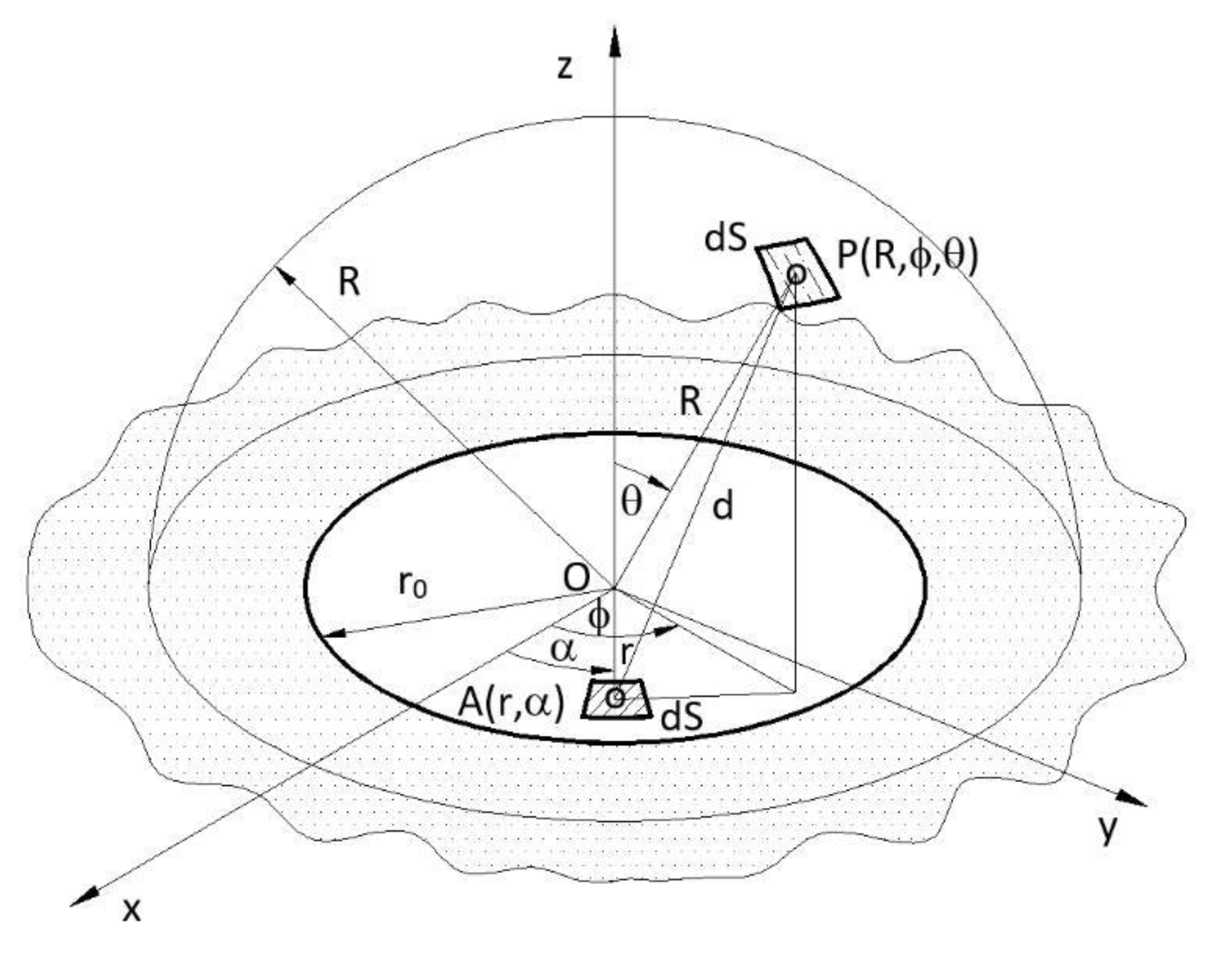
2. Sound Power from Sound Pressure in the Far Field
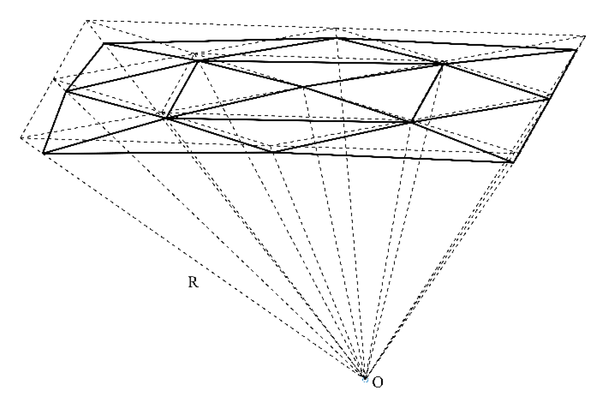
3. New Algorithms for Numerical Surface Integral on a Sphere
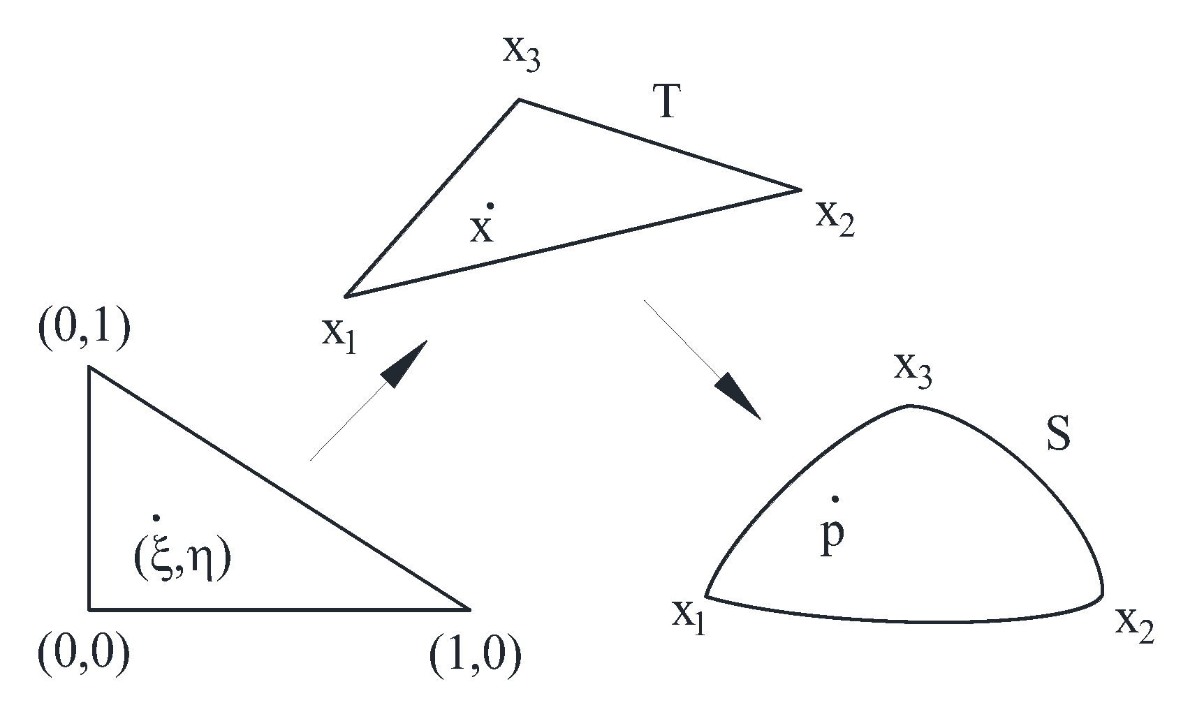
3.1. SQRBF
3.2. ARPIST
4. Examples
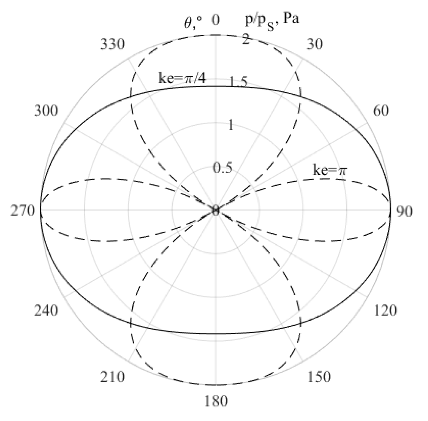
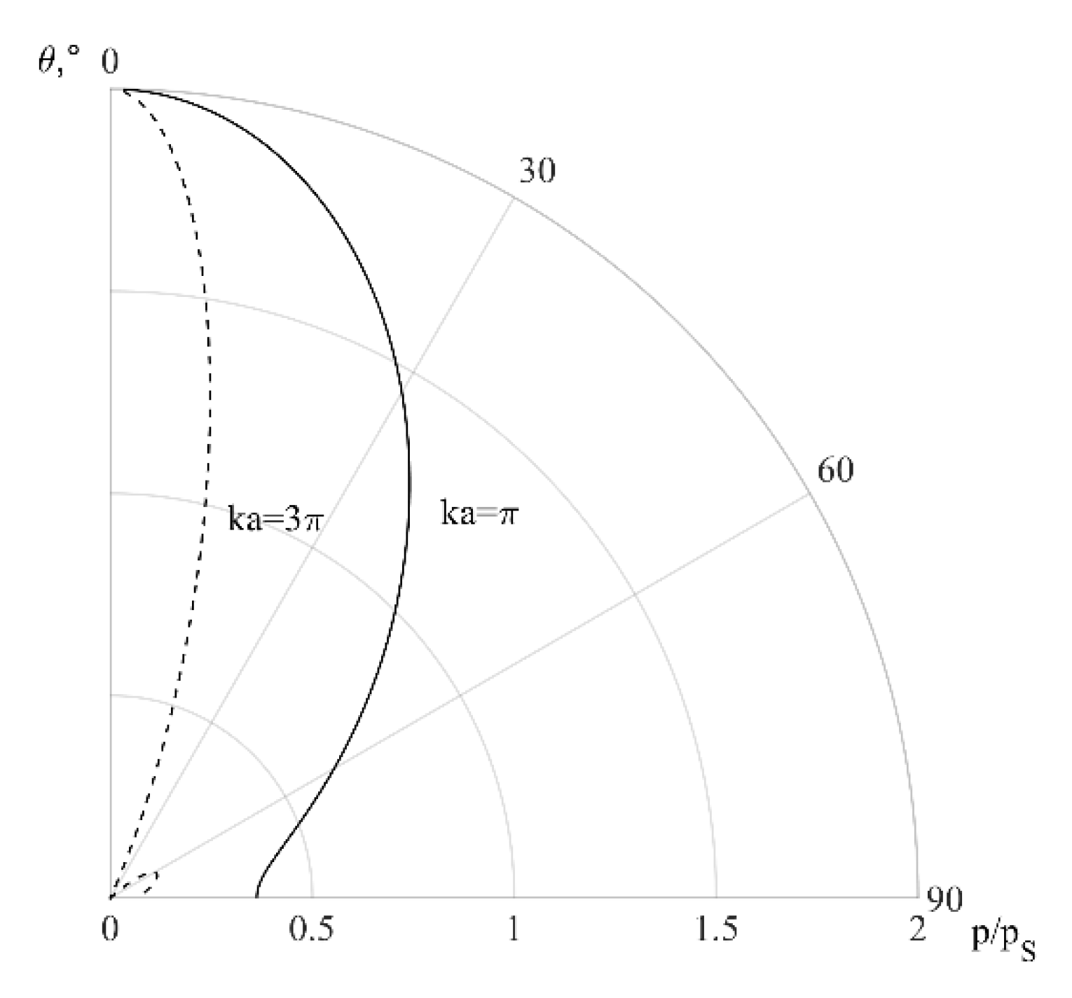
4.1. Sound Pressures on a Sphere in the Far Field
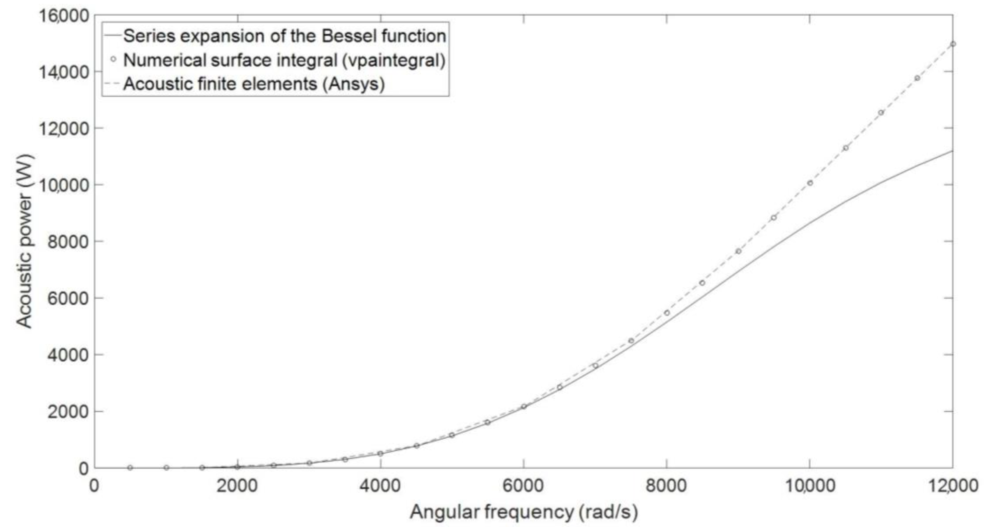
4.2. Sound Power from Sound Pressure, Analytical vs. Numerical Solution
4.3. Sound Power from Sound Pressure, New Algorithms for Numerical Integration on the Sphere
5. Conclusions
- -
- For some sources, it is possible to define integrable functions for the calculation of sound pressure or sound power with an accuracy corresponding to the mathematical simplifications used;
- -
- For other sources, it is not possible to define integrable functions so that numerical surface integration must be used;
- -
- The accuracy of the algorithms ARPIST and SQRBF for numerical integration on a sphere’s surface increases with the increase of its parameters, approaching almost a 0% difference to the reference numerical solution;
- -
- If function values are available at any location on a sphere, ARPIST has a higher accuracy and stability than SQRBF while being faster and easier to implement;
- -
- If function values are available only at user-prescribed locations, SQRBF can directly calculate weights while ARPIST requires high-accuracy scattered data interpolation to obtain function values at these Gaussian quadrature locations from the (coarser sampled) data at the original scattered nodes. Such a procedure reduces the accuracy and increases the calculation time.
Author Contributions
Funding
Data Availability Statement
Conflicts of Interest
References
- Rayleigh, J.W.S. The Theory of Sound; Dower Publications: New York, NY, USA, 1897. [Google Scholar]
- Fahy, F.; Gardonio, P. Sound and Structural Vibration; Radiation, Transmission and Response; Elsevier: Oxford, UK, 2007. [Google Scholar]
- Cunefare, K.A. Effect of Modal Interaction on Sound Radiation from Vibrating Structures. AIAA J. 1992, 30, 2819–2828. [Google Scholar] [CrossRef]
- Herrin, D.W.; Martinus, F.; Wu, T.W.; Seybert, A.F. An assessment of the high frequency boundary element and Rayleigh integral approximations. Appl. Acoust. 2006, 67, 819–833. [Google Scholar] [CrossRef]
- Arenas, J.P. Numerical Computation of the Sound Radiation from a Planar Baffled Vibrating Surface. J. Comput. Acoust. 2008, 16, 321–341. [Google Scholar] [CrossRef]
- Bai, M.R.; Tsao, M. Estimation of sound power of baffled planar sources using radiation matrices. J. Acoust. Soc. Am. 2002, 112, 876–883. [Google Scholar] [CrossRef] [PubMed]
- Kinsler, L.E.; Frey, A.R.; Coppens, A.B.; Sanders, J.V. Fundamentals of Acoustics; John Wiley & Sons, Inc.: New York, NY, USA, 2000. [Google Scholar]
- Junger, M.C.; Feit, D. Sound, Structures, and Their Interaction; MIT Press: London, UK, 1972. [Google Scholar]
- Kirkup, S.M. Computational solution of the acoustic field surrounding a baffled panel by the Rayleigh integral method. Appt. Math. Modelling 1994, 18, 403–407. [Google Scholar] [CrossRef]
- Li, Y.; Jiao, X. ARPIST: Provably Accurate and Stable Numerical Integration over Spherical Triangles. J. Comput. Appl. Math. 2023, 420, 114822. [Google Scholar] [CrossRef]
- Bažant, Z.P.; Oh, B.H. Efficient Numerical Integration on the Surface of a Sphere. ZAMM-Z. Angew. Math. U. Mech. 1986, 66, 37–49. [Google Scholar] [CrossRef]
- Rosca, D. Spherical quadrature formulas with equally spaced nodes on latitudinal circles. Electron. Trans. Numer. Anal. 2009, 35, 148–163. [Google Scholar]
- Shivaram, K.T. Generalised Gaussian Quadrature over a Sphere. Int. J. Sci. Eng. Res. 2013, 4, 1530–1534. [Google Scholar]
- Reeger, J.A.; Fornberg, B. Numerical Quadrature over the Surface of a Sphere. Stud. Appl. Math. 2016, 137, 174–188. [Google Scholar] [CrossRef]
- Fornberg, B.; Martel, J.M. On spherical harmonics based numerical quadrature over the surface of a sphere. Adv. Comput. Math. 2014, 40, 1169–1184. [Google Scholar]
- Reeger, J.A.; Fornberg, B.; Wats, M.L. Numerical quadrature over smooth, closed surfaces. Proc. R. Soc. A 2016, 472, 20160401. [Google Scholar] [CrossRef] [PubMed]
- The Mathworks, Inc. Symbolic Math ToolboxTM, Matlab, R2017a; The Mathworks, Inc.: Natick, MA, USA, 2017. [Google Scholar]
- Reeger, J.A.; Fornberg, B. Numerical quadrature over smooth surfaces with boundaries. J. Comput. Phys. 2018, 355, 176–190. [Google Scholar] [CrossRef]
- Humpherys, J.; Jarvis, T.J.; Evans, E.J. Foundations of Applied Mathematics, Volume I: Mathematical Analysis; SIAM -Society for Industrial and Applied Mathematics: Philadelphia, PA, USA, 2017. [Google Scholar]
- Ma, T.-W. Higher chain formula proved by combinatorics. Electron. J. Comb. 2009, 16, N21. [Google Scholar] [CrossRef] [PubMed]
- Kuntz, H.L.; Hixon, E.L.; Ryan, W.W. The Rayleigh distance and geometric nearfield size of nonplane sound radiators. J. Acoust. Soc. Am. 1983, 74, S82. [Google Scholar] [CrossRef]
- Howard, C.Q.; Cazzolato, B.S. Acoustic Analyses Using Matlab and Ansys; CRC Press: Boca Raton, FL, USA; Taylor & Francis Group: Abingdon, UK, 2015. [Google Scholar]
- Akkaya, N. Acoustic Radiation from Baffled Planar Sources. In A Series Approach; Master of Science, Graduate Faculty of Texas Tech University: Lubbock, TX, USA, 1999. [Google Scholar]
- McLachlan, N.W. Bessel Functions for Engineers; Clarendon Press: Oxford, UK, 1955. [Google Scholar]
- Cools, R. An encyclopedia of cubature formulas. J. Complex. 2003, 19, 445–453. [Google Scholar] [CrossRef]


| Rayleigh Integral | Finite Element Model | ||||
|---|---|---|---|---|---|
| Omega (rad/s) | Min (Pa) | Max (Pa) | Min (Pa) | Max (Pa) | Difference (%) |
| 0 | 0 | 0 | 0 | 0 | 0 |
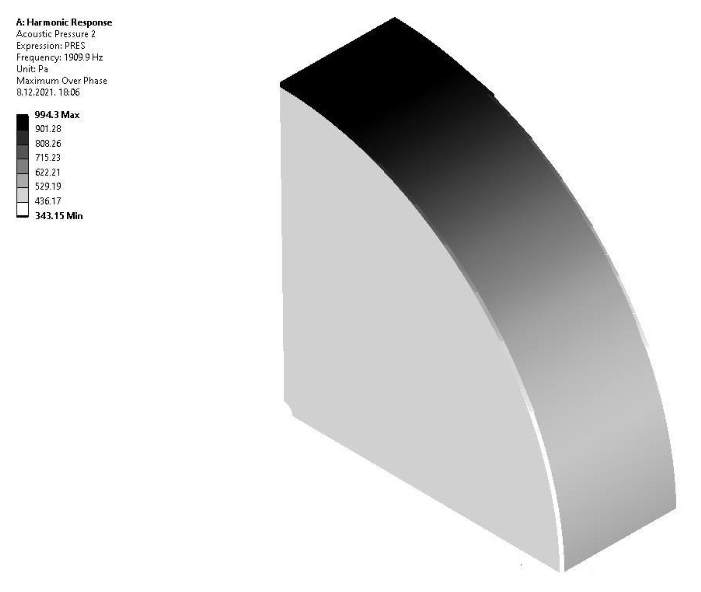
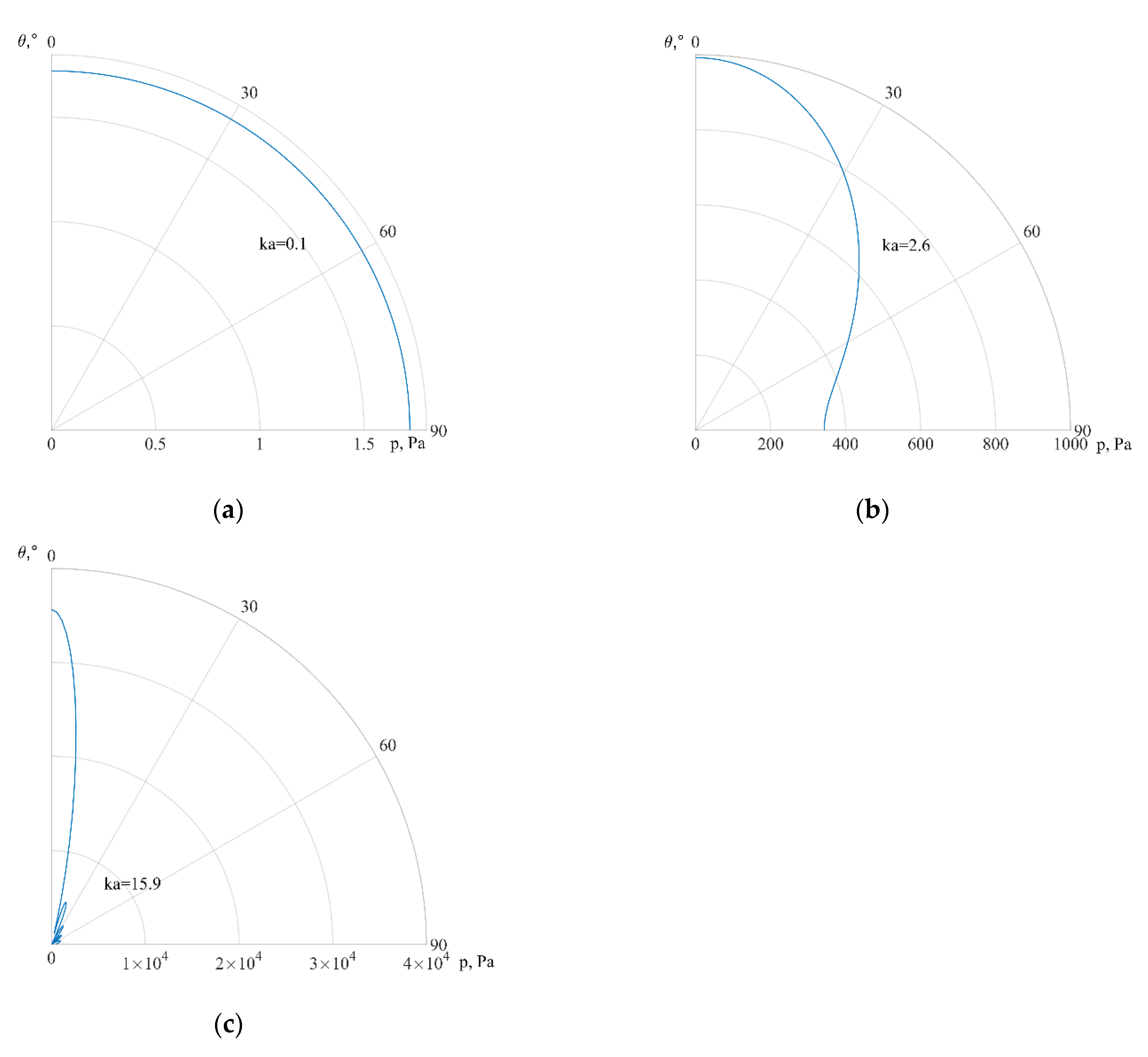
| 500 (Figure 8a) | 1.72 | 1.7227 | 1.7202 | 1.7222 | 0.01% |
| 1000 | 6.8488 | 6.8906 | 6.8484 | 6.8876 | −0.01% |
| 1500 | 15.2927 | 15.5039 | 15.288 | 15.493 | −0.03% |
| 2000 | 26.8973 | 27.5624 | 26.878 | 27.529 | −0.07% |
| 2500 | 41.4499 | 43.0662 | 41.4 | 42.991 | −0.12% |
| 3000 | 58.6822 | 62.0153 | 58.581 | 61.868 | −0.17% |
| 3500 | 78.2751 | 84.4095 | 78.098 | 84.149 | −0.23% |
| 4000 | 99.8631 | 110.2489 | 99.565 | 109.9 | −0.30% |
| 4500 | 123.0401 | 139.5334 | 122.61 | 139.23 | −0.35% |
| 5000 | 147.3655 | 172.263 | 146.96 | 172.05 | −0.28% |
| 5500 | 172.3711 | 208.4376 | 172.05 | 208.35 | −0.19% |
| 6000 | 197.5736 | 248.0571 | 197.3 | 248.06 | −0.14% |
| 6500 | 222.4554 | 291.1214 | 222.02 | 291.32 | −0.20% |
| 7000 | 246.5262 | 337.6306 | 246.07 | 337.79 | −0.19% |
| 7500 | 269.2771 | 387.5844 | 268.89 | 387.54 | −0.14% |
| 8000 | 290.2156 | 440.9828 | 289.84 | 441.57 | −0.13% |
| 8500 | 308.8679 | 497.8258 | 308.49 | 499.1 | −0.12% |
| 9000 | 324.7868 | 558.1131 | 324.62 | 559.18 | −0.05% |
| 9500 | 337.5587 | 621.8448 | 337.47 | 622.5 | −0.03% |
| 10,000 | 346.8109 | 689.0206 | 346.26 | 689.36 | −0.16% |
| 10,500 | 352.2176 | 759.6405 | 351.73 | 761.55 | −0.14% |
| 11,000 | 353.5478 | 833.7043 | 352.82 | 839.64 | −0.21% |
| 11,500 | 350.4603 | 911.2119 | 350.1 | 915.1 | −0.10% |
| 12,000 (Figure 8b) | 342.9279 | 992.1631 | 343.01 | 993.95 | 0.02% |
| ω (rad/s) | Π (W) Numerical Integral of Function of One Scalar θ, Equation (30) | Π (W) Numerical Quadrature – SQRBF, 200 Nodes | Difference (%) | Π (W) Numerical Quadrature – SQRBF, 2500 Nodes | Difference (%) | Π (W) Numerical Quadrature – ARPIST Degree-4, 1920 q.n. | Difference (%) |
|---|---|---|---|---|---|---|---|
| 0 | 0 | 0 | - | 0 | - | 0 | - |
| 500 | 0.1396 | 0.1378 | −1.29 | 0.1394 | −0.14 | 0.1396 | 0 |
| 1000 | 2.2203 | 2.1918 | −1.28 | 2.2166 | −0.17 | 2.2203 | 0 |
| 1500 | 11.1269 | 10.9849 | −1.28 | 11.1084 | −0.17 | 11.1269 | 0 |
| 2000 | 34.6708 | 34.2310 | −1.27 | 34.6138 | −0.16 | 34.6708 | 0 |
| 2500 | 83.1151 | 82.0690 | −1.26 | 82.9798 | −0.16 | 83.1152 | 1.20 × 10⁻⁴ |
| 3000 | 168.5471 | 166.4460 | −1.25 | 168.2759 | −0.16 | 168.5472 | 5.93 × 10⁻⁵ |
| 3500 | 304.1349 | 300.3781 | −1.24 | 303.6523 | −0.16 | 304.1350 | 3.29 × 10⁻⁵ |
| 4000 | 503.3099 | 497.1912 | −1.22 | 502.5243 | −0.16 | 503.3099 | 0 |
| 4500 | 778.9220 | 769.6002 | −1.20 | 777.7295 | −0.15 | 778.9221 | 1.28 × 10⁻⁵ |
| 5000 | 1142.4167 | 1128.9878 | −1.18 | 1140.7060 | −0.15 | 1142.4169 | 1.75 × 10⁻⁵ |
| 5500 | 1603.0804 | 1584.6158 | −1.15 | 1600.7400 | −0.15 | 1603.0807 | 1.87 × 10⁻⁵ |
| 6000 | 2167.4006 | 2143.0009 | −1.13 | 2164.3260 | −0.14 | 2167.4011 | 2.31 × 10⁻⁵ |
| 6500 | 2838.5769 | 2807.4298 | −1.10 | 2834.6789 | −0.14 | 2838.5774 | 1.76 × 10⁻⁵ |
| 7000 | 3616.2145 | 3577.6519 | −1.07 | 3611.4275 | −0.13 | 3616.2152 | 1.94 × 10⁻⁵ |
| 7500 | 4496.2212 | 4449.7712 | −1.03 | 4490.5101 | −0.13 | 4496.2221 | 2 × 10⁻⁵ |
| 8000 | 5470.9154 | 5416.3455 | −1.00 | 5464.2817 | −0.12 | 5470.9164 | 1.83 × 10⁻⁵ |
| 8500 | 6529.3439 | 6466.6908 | −0.96 | 6521.8304 | −0.12 | 6529.3451 | 1.84 × 10⁻⁵ |
| 9000 | 7657.7965 | 7587.3790 | −0.92 | 7649.4888 | −0.11 | 7657.7978 | 1.70 × 10⁻⁵ |
| 9500 | 8840.4899 | 8762.9028 | −0.88 | 8831.5163 | −0.10 | 8840.4913 | 1.58 × 10⁻⁵ |
| 10,000 | 10,060.3883 | 9976.4759 | −0.83 | 10,050.9165 | −0.09 | 10,060.3898 | 1.49 × 10⁻⁵ |
| 10,500 | 11,300.1169 | 11,210.9248 | −0.79 | 11,290.3480 | −0.09 | 11,300.1184 | 1.33 × 10⁻⁵ |
| 11,000 | 12,542.9196 | 12,449.6266 | −0.74 | 12,533.0797 | −0.08 | 12,542.9211 | 1.20 × 10⁻⁵ |
| 11,500 | 13,773.6090 | 13,677.4406 | −0.70 | 13,763.9385 | −0.07 | 13,773.6103 | 9.44 × 10⁻⁶ |
| 12,000 | 14,979.4566 | 14,881.5836 | −0.65 | 14,970.1981 | −0.06 | 14,979.4576 | 6.68 × 10⁻⁶ |
| m | n | N | Π (W) SQRBF | Difference from Equation (30) (%) | (Elem. Num. × 6 Quad. Nodes) | Π (W) ARPIST (Degree-4) | Difference from Equation (30) (%) |
|---|---|---|---|---|---|---|---|
| ω = 4000 rad/s | |||||||
| 13 | 500 | 7000 | 503.0846 | −0.04 | |||
| 13 | 800 | 8000 | 503.4717 | 0.03 | 7680 | 503.3099 | 0 |
| 13 | 1000 | 10,000 | 503.1052 | −0.04 | |||
| 13 | 1000 | 15,000 | 503.1452 | −0.03 | |||
| 13 | 1000 | 20,000 | 503.3092 | −1.39 × 10⁻⁵ | |||
| ω = 12,000 rad/s | |||||||
| 13 | 1000 | 20,000 | 14,979.4492 | −4.94 × 10⁻⁷ | 17,280 | 14,979.4566 | 0 |
| ω = 72,000 rad/s (Figure 8c) | |||||||
| 13 | 1000 | 20,000 | 478,691.0053 | −4.57 × 10⁻⁶ | 17,280 | 478,691.1647 | 2.87 × 10⁻⁵ |
Disclaimer/Publisher’s Note: The statements, opinions and data contained in all publications are solely those of the individual author(s) and contributor(s) and not of MDPI and/or the editor(s). MDPI and/or the editor(s) disclaim responsibility for any injury to people or property resulting from any ideas, methods, instructions or products referred to in the content. |
© 2023 by the authors. Licensee MDPI, Basel, Switzerland. This article is an open access article distributed under the terms and conditions of the Creative Commons Attribution (CC BY) license (https://creativecommons.org/licenses/by/4.0/).
Share and Cite
Piličić, S.; Skoblar, A.; Žigulić, R.; Traven, L. Applying New Algorithms for Numerical Integration on the Sphere in the Far Field of Sound Pressure. Acoustics 2023, 5, 999-1015. https://doi.org/10.3390/acoustics5040057
Piličić S, Skoblar A, Žigulić R, Traven L. Applying New Algorithms for Numerical Integration on the Sphere in the Far Field of Sound Pressure. Acoustics. 2023; 5(4):999-1015. https://doi.org/10.3390/acoustics5040057
Chicago/Turabian StylePiličić, Stjepan, Ante Skoblar, Roberto Žigulić, and Luka Traven. 2023. "Applying New Algorithms for Numerical Integration on the Sphere in the Far Field of Sound Pressure" Acoustics 5, no. 4: 999-1015. https://doi.org/10.3390/acoustics5040057