The Spherical Harmonic Family of Beampatterns

Abstract

The free space solution to the wave equation in spherical coordinates is well known as a separable product of functions. Re-examination of these functions, particularly the sums of spherical Bessel and harmonic functions, reveals behaviors which can produce a range of useful beampatterns from radially symmetric sources. These functions can be modified by several key parameters which can be adjusted to produce a wide-ranging family of beampatterns, from the axicon Bessel beam to a variety of unique axial and lateral forms. We demonstrate that several special properties of the simple sum over integer orders of spherical Bessel functions, and then the sum of their product with spherical harmonic functions specifying the free space solution, lead to a family of useful beampatterns and a unique framework for designing them. Examples from a simulation of a pure tone 5 MHz ultrasound configuration demonstrate strong central axis concentration, and the ability to modulate or localize the axial intensity with simple adjustment of the integer orders and other key parameters related to the weights and arguments of the spherical Bessel functions.

1. Introduction

In the design of coherent imaging systems using optical or ultrasound excitation, there has been a longstanding interest in the behavior of beampatterns. One active area of interest is the field of localized waves or weakly diffracting beams [1]. These include the Bessel beam [2,3], the X-wave [4], and the needle pulse [5]. Ultrasound imaging systems with phased array transducers traditionally rely on focusing and apodization strategies to achieve high spatial resolution in the transverse direction [6,7] and in this context a key consideration is the beamwidth as a function of depth, along with the minimization of sidelobes [8,9]. A useful concept in designing beampatterns is the Fourier transform relation that applies to the field on a source plane and at some farfield or focal depth [10,11]. This, combined with related approximations, enables the specification and selection of beams from practical systems [12].

In this paper, an alternative framework is examined for specifying radially symmetric beampatterns, by using interpretations of the free-space separable solution to the Helmholtz equation. In particular, the sum over integer orders of the spherical Bessel and harmonic (SBH) product terms has unique properties that produce a number of useful implementations. First, localized central axis beams can be produced, with a variety of axial profiles linked directly to the selection of the integer orders. Second, some other key parameters related to the weights and arguments of the functions, can be specified to create a family of beampatterns ranging from the classical Bessel beam produced by an optical axicon of limited aperture [2,3] to a range of axial and transverse patterns. These beampatterns can be adjusted within the framework of the sums of SBH terms and without necessary recourse to traditional treatments of focusing and Fourier transform operations. Examples are provided from theoretical treatments of a 5 MHz flat radially symmetric transducer.

2. Theory

2.1. General Solution

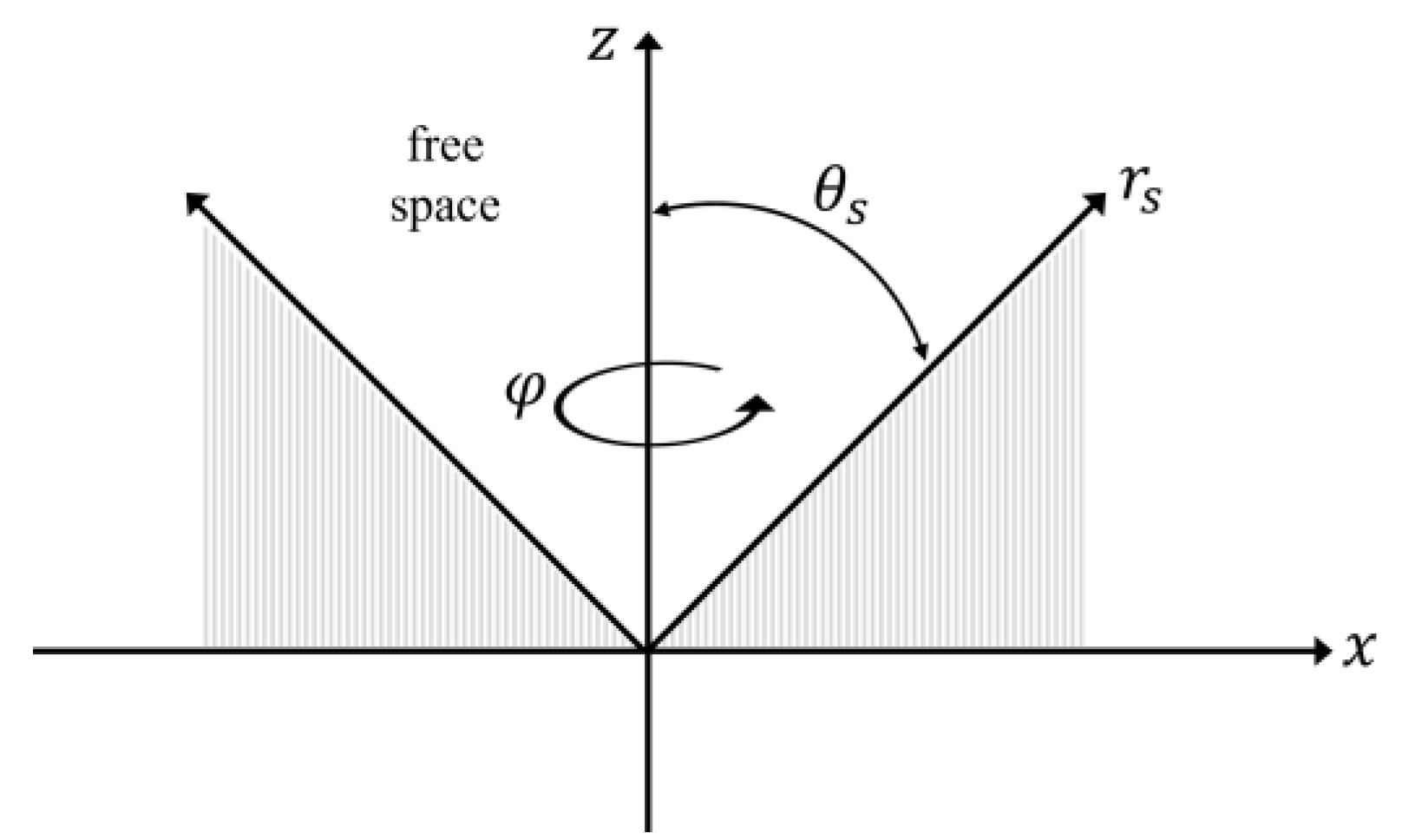
Let us reconsider the classic separable solution for monochromatic waves in a spherical coordinate system, initially assuming a source surface that is conically shaped with prescribed boundary conditions radiating into the interior free space within a cone (Figure 1).

In spherical coordinates, the free space Helmholtz equation is known to be separable [13,14,15,16] and can be written as:

$$A\left(r,\theta ,\phi \right)={\displaystyle \sum _{n=0}^{\infty }{\displaystyle \sum _{m=-\ell }^{\ell }\left(a_{nm}{j}_n\left(kr\right)+b_{nm}{y}_n\left(kr\right)\right)Y_n^m\left(\theta ,\phi \right)}}.$$

(1)

Here, $j_{\iota }\left(kr\right)$ and $y_{\iota }\left(kr\right)$ are the spherical Bessel functions, $Y_{\iota }^m\left(\theta ,\phi \right)$ are the spherical harmonics [17], and $a_{nm}$ and $b_{nm}$ are the amplitudes assigned to each of the functions. In the summation limits, n represents the integer orders of the spherical Bessel functions and m represents the finite number of azimuthal angle orders. Note that this form provides general solutions, and requires boundary conditions to be specified in any specific case [18,19].

Now to simplify these, let us restrict our examinations to the solutions that are finite at r = 0, are symmetric about $\phi$, and are comprised of a limited sum of integer orders up to a maximum of N:

$$A\left(r,\theta \right)={\displaystyle \sum _{n=0}^N{a}_n{j}_n\left(kr\right)Y_n^0\left(\theta \right)}.$$

(2)

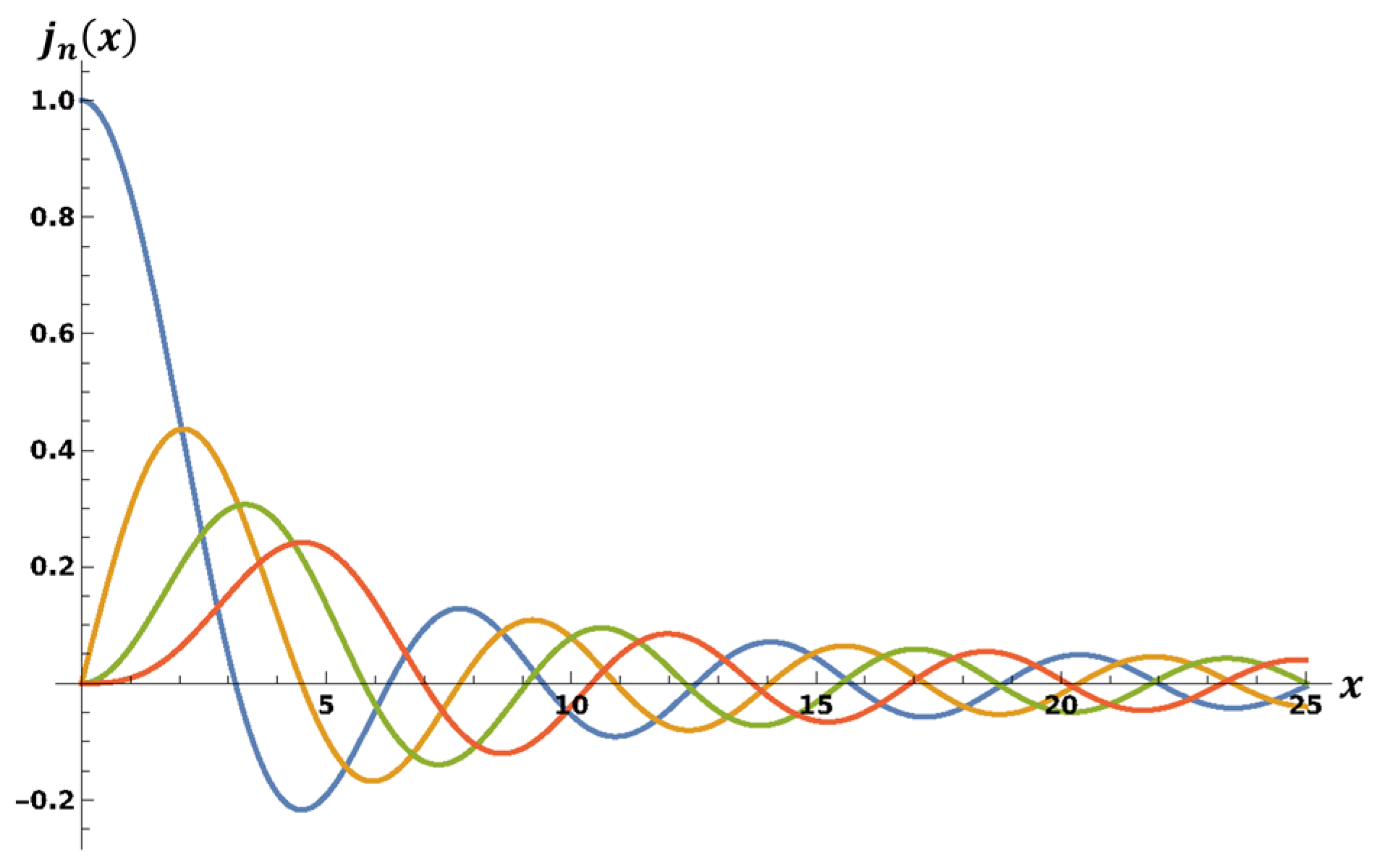
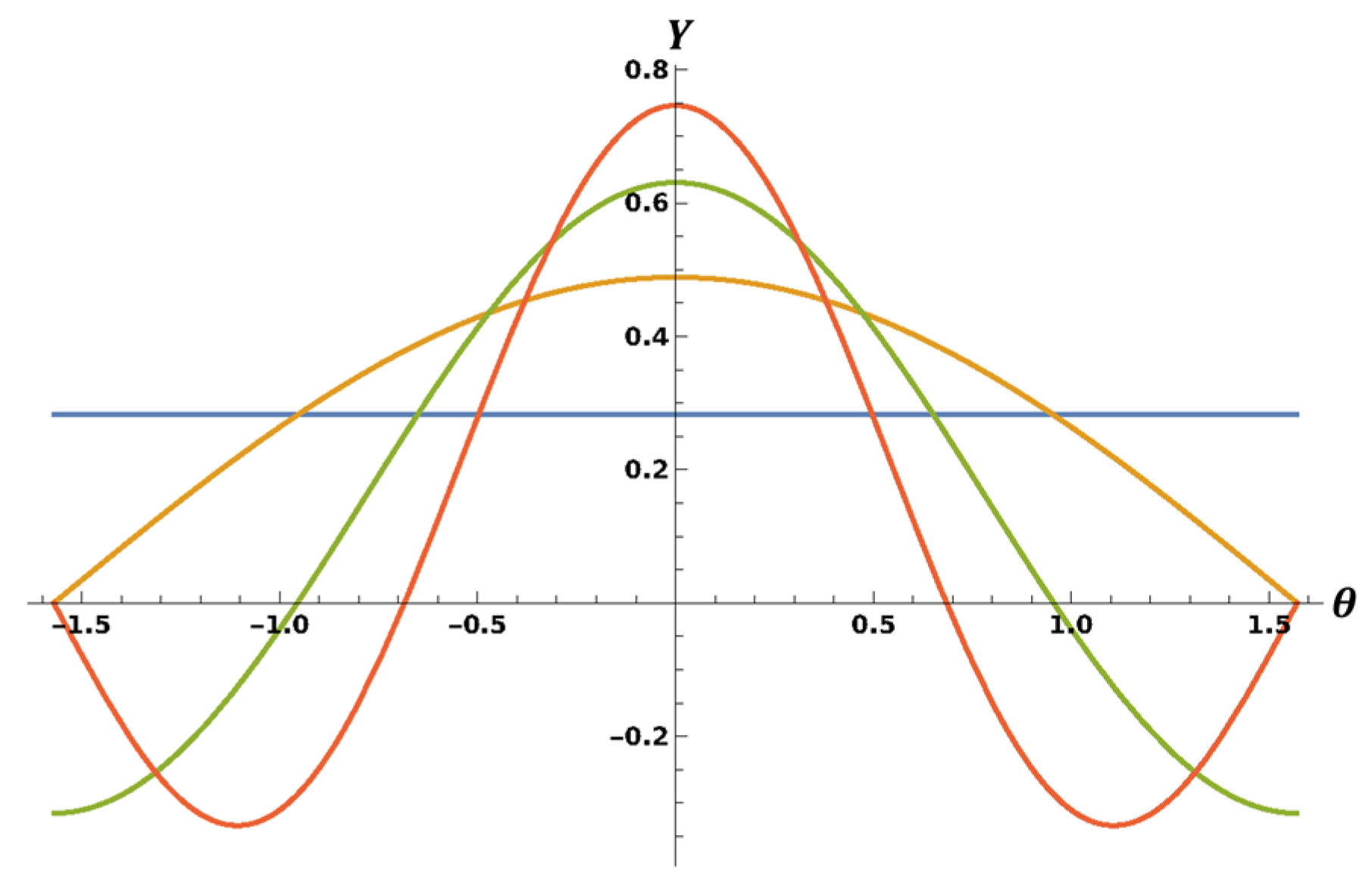
To visualize the different terms, Figure 2 shows the first few spherical Bessel functions of increasing order, and Figure 3 displays several low order spherical harmonic functions Y as a function of $\theta$.

Now, consistent with the classical treatments of Green’s functions and the RayleighSommerfield integral theorems [20,21], we may reinterpret Equations (1) and (2) as a design specification on boundary conditions. If a single spherical Bessel function $j_n\left(kr\right)$ can be excited as a source function across the surface of the cone shown in Figure 1, in steady state, the corresponding product of that function with $Y_n\left(\theta \right)$ will be uniquely generated in the interior free space region. Furthermore, the principle of superposition applies directly as indicated in Equation (2), meaning that if we can simultaneously establish the sum of spherical Bessel functions on the surface of the cone, the resulting field as a function of $\theta$ will be composed of the summation over all orders of corresponding $Y_n$. Here, we are not talking about summation over frequency $\omega$ (or wavenumber k), but instead summation over integer orders of spherical Bessel functions of the same frequency. Thus, a closer examination of summations is warranted.

2.2. Special Properties of Sums of Spherical Bessel Functions

Because of the asymptotic limit of $j_n\left(x\right)$ being equal to [17], effectively the long tails of any group of four successive orders of equal amplitude and phase will trend towards zero. Meanwhile the early maximum or peak of each order n is progressively delayed from the origin and decreases as $\sqrt{n}$. Therefore, the summation series has properties that, in the context of signal processing, appear to be useful as an interpolation function for a sampled, bandlimited signal. Specifically:

$$j_n\left(x\right)\to \sin \left(x-\frac{1}{2}n\pi \right)/x \mathrm{for} x\to \infty$$

(3)

$${\displaystyle \sum _{n=1}^N{j}_n\left(x\right)\cong \{\begin{array}{cc}\frac{\sqrt{\pi /2}}{\sqrt{x}}& 0<x\le N\\ 0& x>N\end{array}}$$

(4)

$${\displaystyle \sum _{n=1}^N\sqrt{n}{j}_n\left(x\right)\cong \{\begin{array}{cc}\sqrt{\pi /2}& 0<x\le N\\ 0& x>N\end{array}}$$

(5)

$${\displaystyle \sum _{n=1}^{N}f\left(n\right)\left(\sqrt{n}{j}_n\left(x\right)\right)\cong \{\begin{array}{cc}\left(\sqrt{\pi /2}\right)f\left(x\right)& 0<x\le N\\ 0& x>N\end{array}}$$

(6)

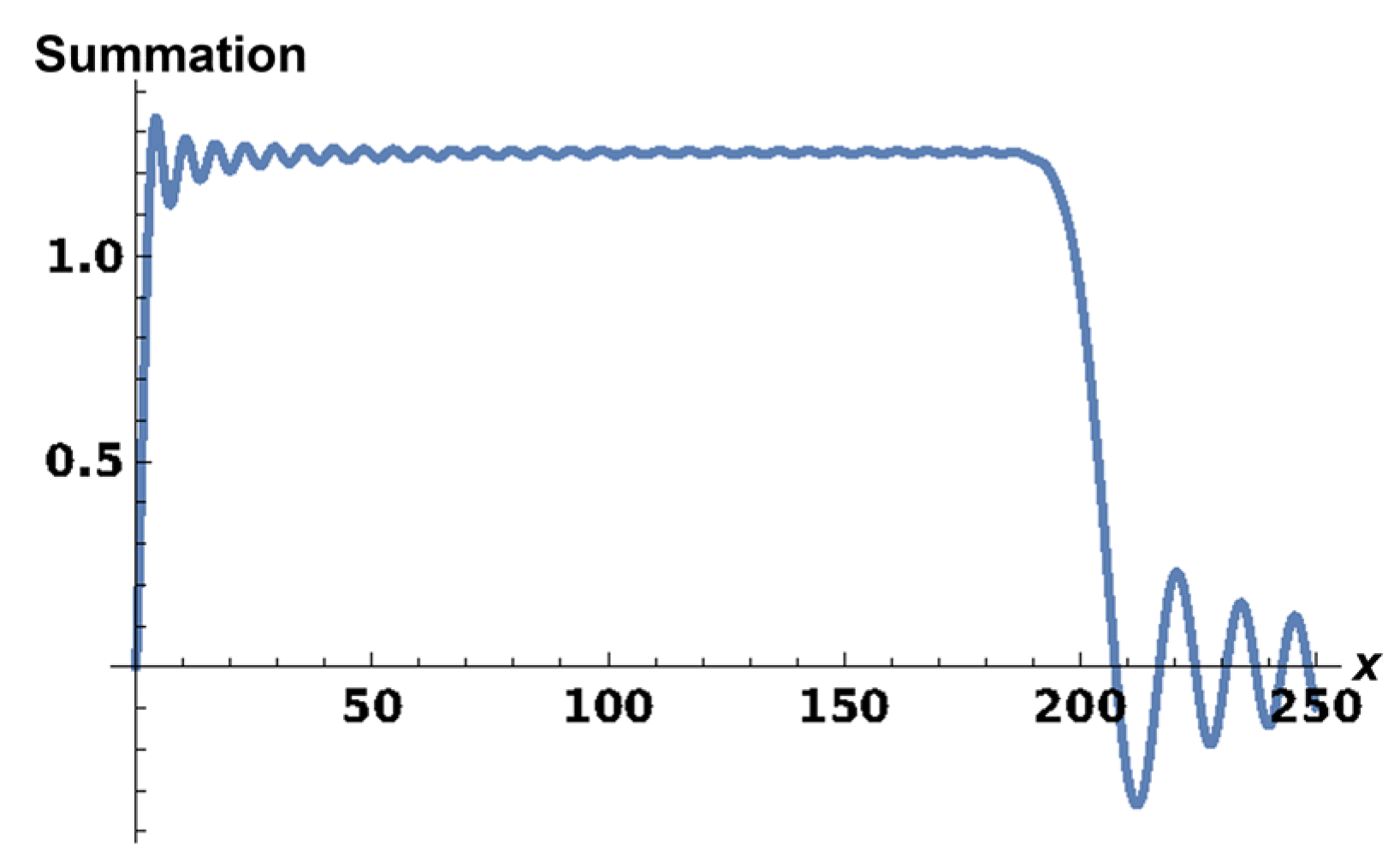
Thus, any arbitrary (well-behaved, bandlimited) sampled function can be reconstructed approximately as the sum of spherical Bessel functions. The sum described by Equation (5) is shown in Figure 4, resembling a band limited window function over the range of 0 < x < 200.

Additionally, the issues of apodization and truncation of a source can be recast by the apodization and termination of the series. This representation is similar to the Neumann series of Bessel functions [22], albeit with simpler interpretation of the coefficients. An example is shown in Figure 5. The advantages of using the spherical Bessel functions as interpolation functions in this way is that each order is matched to corresponding spherical harmonic functions, enabling the full description of a wave field in three-dimensional free space as a precise analytical expression. Furthermore, in the case of the active area of a transducer surface, each integer order or group of orders define a radial region on the transducer and in the wave produced in free space. These properties will be illustrated in the subsequent sections.

2.3. Modifications via Imaginary Shift in Coordinates

Alonso et al. considered a modification to the classical solution of spherical harmonic functions in terms of an offset consisting of a purely imaginary constant [23]. Including a simple offset in the argument of Equation (1) is also a valid solution to the wave equation, thus $z\to z+iq$ is substituted in all expressions, where i is the imaginary unit index and q is an arbitrary constant. This imaginary parameter can be shown to remap the angular spectrum in a geometrical transformation around the unit circle defined by $\theta$. Practically speaking, this parameter q is then used as a parameter which can significantly alter the beampattern and its angular spectrum.

2.4. Other Simple Modifications and Properties

In addition to the use of the $a_n$ in Equation (2) for apodization as shown in Figure 5, another tactic for implementation at the transducer surface is to prescribe the $a_n$ as a modulation with respect to the integer orders n. This effectively changes the angular spectrum and the spatial location of the peak region of the beampattern in free space. In the context of Equation (1), we note that both the $j_n$ and the $Y_n^0\left(\theta =\pi /2\right)$ have a natural oscillation, with values repeating or approximately repeating with ascending n, every n = 4 integer orders. Thus, a modulation function such as:

$$a_n=\cos \left[2\pi \left(\frac{n}{N_{\mathrm{mod}}}\right)+\varphi \right]$$

(7)

will influence the summation, and when N_mod = 4, this imposed modulation of integer orders matches the natural modulation of the $j_n$ and $Y_n^0$.

3. Methods

Calculations of the free space fields were performed using Mathematica (Version 13.0.1, Wolfram Research, Champaign, IL, USA) and using a working precision of 20 or more decimal places in all calculations.

In all the following examples, we specify conditions related to a 5 MHz medical ultrasound system, with wavelength approximately 0.3 mm and with the summation of spherical Bessel integer orders n up to 200. This upper limit kr_max = 200 corresponds to an active high amplitude transducer radius of approximately 10 mm, with a residual decay beyond that radius. We also assume a flat transducer so that the cone angle of Figure 1 is set to $\pi /2$; this models the use of a conventional piston transducer, albeit with active control of the amplitude and phase of the excitation across the transducer.

4. Results

For the simple summation of Equation (2) up to n = 200, we examine the cases referred to in Equations (4) and (5); the unweighted sum (a_n = 1) and the square root weighted sum (a_n = n^1/2). These display a strong central axis amplitude with oscillations in the radial direction as shown in Figure 6.

Axial plots of these are shown in Figure 7.

Transverse cuts of these two cases at 8 mm axial range are shown in Figure 8. Despite the difference in axial amplitudes (above), both of the transverse beampatterns are a close fit to the Bessel function of zero order: J₀[kx], thus resembling the classical Bessel beam described by Durnin as implemented within the framework of the optical axicon [2,3].

Next, we turn to variation in the q parameter. With all other factors held the same as in Figure 6 (top), the imaginary offset is added to the z (axial) coordinate, q = 1/2 and 1, respectively within the arguments of Equation (2). It should be noted that the addition of the imaginary q offset does change the amplitudes and phases of the spherical Bessel functions at the active transducer, introducing an enhanced source strength near the origin, as shown in Figure 9.

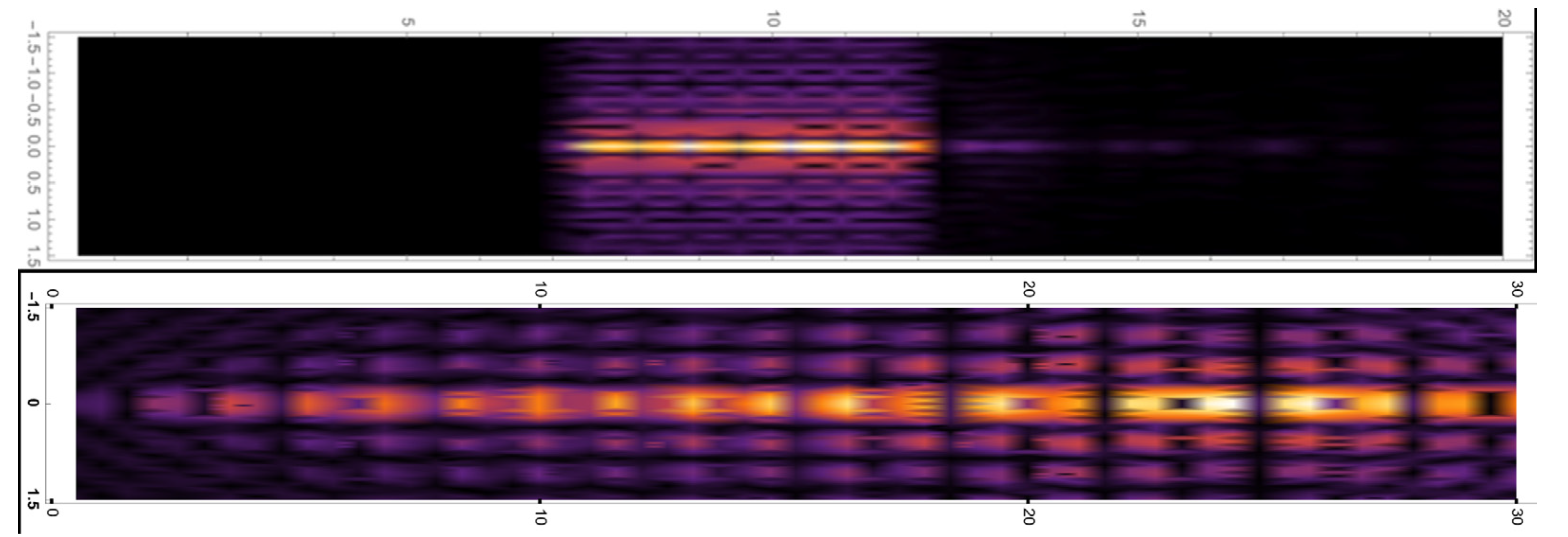
Next, we examine some alternative modifications. The localization property of the summation is illustrated in Figure 10 (top), where only the sum from integer orders 150 to 250 are activated. This translates into a localized area of axial strength from 7 to 12 mm from the transducer surface. An oscillatory term is added to the coefficients and shown in Figure 10 (bottom) using Equation (7) with N_mod = 2.5. This modulates the amplitudes of the integer orders within the sum, and thereby serves as a rough equivalent to changing the angle of incidence in conical optical axicon configurations.

Finally, a single integer order of 199 is shown in Figure 11, including the offset parameter of q = 1/2. We note an extended centralized beampattern and this has some resemblance to Figure 1 of Cizmár and Dholakia [24] which demonstrates their annular source axicon.

5. Discussion and Conclusions

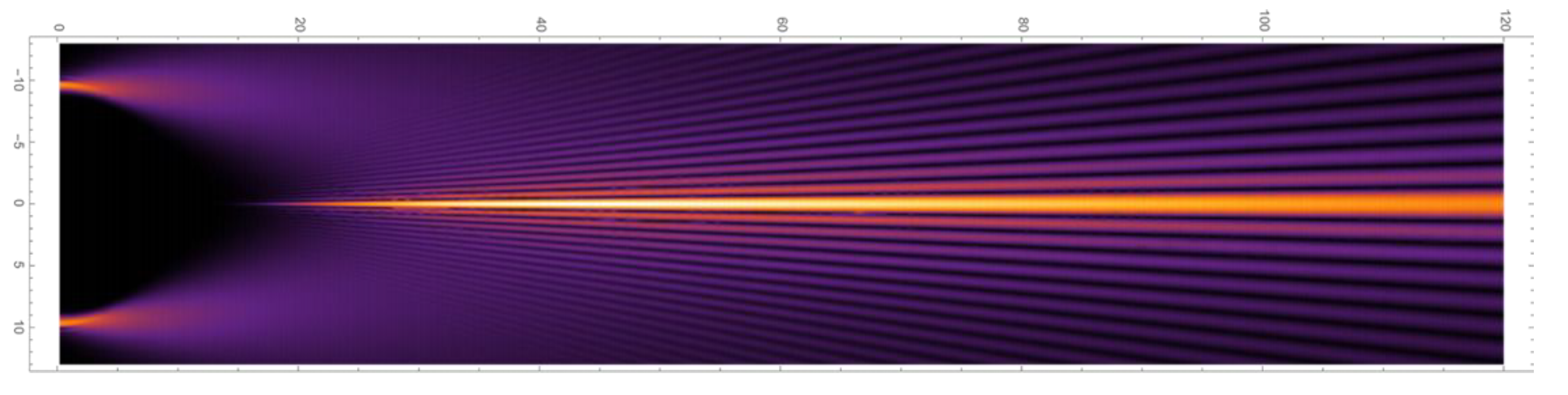
The free space sums of SBH functions in Equation (2) are of particular interest along the central axis ($\theta =0$) and in the case of a flat piston source, along the source plane ($\theta =\pi /2$). Along the central axis, the spherical harmonic functions $Y_n^o\left(0\right)$ increase approximately proportional to $\sqrt{n}$ with increasing n. Thus, if in Equation (2), we set the $a_n=1$, the resulting terms resemble Equation (5), and then the central axis amplitude is uniform out to the limit of $kz=N_{\max }$, as demonstrated in Figure 6 (lower) and Figure 7 (lower). The flat piston source corresponds to $\theta =\pi /2$, and is of practical interest for the specification of the source excitation. As mentioned previously, and as can be seen at the extreme edges of Figure 3, the $Y_n^o\left(\pi /2\right)$ will oscillate between positive, zero, negative, and zero values, repeatedly with a period of 4n. This modulates the sum of product terms and generally increases the relative weights of the source for $kr>N_{\max }$ beyond those expected from the examples of the sum of unweighted $j_n$. In addition, the imaginary offset q tends to produce at the source plane a significantly stronger amplitude for the outer region of $kr>N_{\max }$. Practically, this means that the active source area needs an extended outer region and additional apodization functions may be included to restrict the active source region. Furthermore, consideration of the angular spectrum [23] and the asymptotic forms of the SBH solutions [25] indicate that fields similar to that shown in Figure 11 will have non-negligible propagation at angles near $\theta =\pi /2$, which would require an unreasonably large source radius to approximate. Utilizing a source angle slightly less than $\pi /2$, effectively a cone surface at small angle with the z axis, will help to mitigate this. We also note that the spherical Bessel functions are related to simple Bessel functions of half-integer order [22], thus Equations (1)–(6) could be rewritten in an alternative form using this substitution.

Limitations of this study are that only steady state monochromatic examples are considered. Transient behavior with broad band imaging pulses remains to be studied, and are left for future work. Additionally, practical effects of transducer element size and spacing in phased arrays will have an effect on the resulting beampatterns. These will also require further research with specific parameters.

Overall, the SBH framework presents a number of useful options for the generation of radially symmetric beampatterns, by recognizing the special properties of the sums of spherical Bessel functions and their product with spherical harmonic functions at different angles. This framework recasts some of the traditional treatments of apodization, focusing, and design specifications around the summation properties including interpolation, localization, and modulation.

References

- Hernández-Figueroa, H.E.; Zamboni-Rached, M.; Recami, E. Localized Waves; IEEE Press: Hoboken, NJ, USA, 2008. [Google Scholar]
- Durnin, J. Exact solutions for nondiffracting beams. I. The scalar theory. JOSA 1987, 4, 651–654. [Google Scholar] [CrossRef]
- Durnin, J.; Miceli, J., Jr.; Eberly, J.H. Diffraction-free beams. Phys. Rev. Lett. 1987, 58, 1499–1501. [Google Scholar] [CrossRef] [PubMed]
- Lu, J.Y.; Greenleaf, J.F. Nondiffracting X waves-exact solutions to free-space scalar wave equation and their finite aperture realizations. IEEE Trans. Ultrason. Ferroelectr. Freq. Control 1992, 39, 19–31. [Google Scholar] [CrossRef]
- Parker, K.J.; Chen, S.; Alonso, M.A. The ultrasound needle pulse. IEEE Trans. Ultrason. Ferroelectr. Freq. Control 2017, 64, 1045–1049. [Google Scholar] [CrossRef] [PubMed]
- Cobbold, R.S.C. Foundations of Biomedical Ultrasound; Oxford University Press: New York, NY, USA, 2007. [Google Scholar]
- Szabo, T.L. Diagnostic Ultrasound Imaging: Inside Out; Elsevier Academic Press: Burlington, MA, USA, 2004. [Google Scholar]
- Parker, K.J. Correspondence: Apodization and windowing functions. IEEE Trans. Ultrason. Ferroelectr. Freq. Control 2013, 60, 1263–1271. [Google Scholar] [CrossRef] [PubMed]
- Parker, K.J. Correspondence: Apodization and windowing eigenfunctions. IEEE Trans. Ultrason. Ferroelectr. Freq. Control 2014, 61, 1575–1579. [Google Scholar] [CrossRef] [PubMed]
- Williams, E.G. Fourier Acoustics: Sound Radiation and Nearfield Acoustical Holography; Academic Press: San Diego, CA, USA, 1999. [Google Scholar]
- Goodman, J.W. Introduction to Fourier Optics, 3rd ed.; Roberts & Co.: Englewood, CO, USA, 2005. [Google Scholar]
- Sheppard, C.J.R.; Alonso, M.A.; Moore, N.J. Localization measures for high-aperture wavefields based on pupil moments. J. Opt. A Pure Appl. Opt. 2008, 10, 033001. [Google Scholar] [CrossRef]
- Boyer, C.P.; Kalnins, E.G.; Miller, W. Symmetry and separation of variables for the Helmholtz and Laplace equations. Nagoya Math. J. 1976, 60, 35–80. [Google Scholar] [CrossRef] [Green Version]
- Baddour, N. Multidimensional wave field signal theory: Mathematical foundations. AIP Adv. 2011, 1, 022120. [Google Scholar] [CrossRef] [Green Version]
- Baddour, N. Multidimensional wave field signal theory: Transfer function relationships. Math. Probl. Eng. 2012, 2012, 478295. [Google Scholar] [CrossRef]
- Baddour, N. The derivative-free Fourier shell identity for photoacoustics. Springerplus 2016, 5, 1597. [Google Scholar] [CrossRef] [PubMed] [Green Version]
- Abramowitz, M.; Stegun, I.A. Handbook of Mathematical Functions with Formulas, Graphs, and Mathematical Tables; U.S. Government Publishing Office: Washington, WA, USA, 1964; p. 1046.
- Morse, P.M.; Ingard, K.U. Theoretical Acoustics, Chapter 7; Princeton University Press: Princeton, NJ, USA, 1987. [Google Scholar]
- Wang, Z.; Wu, S.F. Helmholtz equation-least-squares method for reconstructing the acoustic pressure field. J. Acoust. Soc. Am. 1997, 102, 2020–2032. [Google Scholar] [CrossRef]
- Wolf, E.; Marchand, E.W. Comparison of the Kirchhoff and the Rayleigh–Sommerfeld theories of diffraction at an aperture. JOSA 1964, 54, 587–594. [Google Scholar] [CrossRef]
- Pierce, A.D. Acoustics: An Introduction to Its Physical Principles and Applications; McGraw-Hill Book Co.: New York, NY, USA, 1981. [Google Scholar]
- Watson, G.N. A Treatise on the Theory of Bessel Functions, Chapter XVI; Cambridge University Press: London, UK, 1922. [Google Scholar]
- Alonso, M.A.; Borghi, R.; Santarsiero, M. New basis for rotationally symmetric nonparaxial fields in terms of spherical waves with complex foci. Opt. Express 2006, 14, 6894–6905. [Google Scholar] [CrossRef] [PubMed]
- Cizmár, T.; Dholakia, K. Tunable Bessel light modes: Engineering the axial propagation. Opt. Express 2009, 17, 15558–15570. [Google Scholar] [CrossRef] [PubMed]
- Devaney, A.J.; Wolf, E. Multipole expansions and plane wave representations of the electromagnetic field. J. Math. Phys. 1974, 15, 234–244. [Google Scholar] [CrossRef]
Figure 1.
Geometry for expansion of spherical waves within a cone of polar angle , and with the surface of the cone being an active source capable of generating spatial distributions in the form of spherical Bessel functions and sums of spherical Bessel functions. The azimuthal angle is , the radial coordinate lies on the active source, and z represents the zenith direction.
Figure 2.
The first four orders of spherical Bessel functions jn(x) as a function of argument x (abscissa). Note that each initial maximum is successively delayed and diminished, while the asymptotes can create out-of-phase cancellation The peaks from left to right correspond to integer orders 0 (blue line), 1 (yellow line), 2 (green line), and 3 (orange line).
Figure 3.
First four orders of the spherical harmonic functions as a function of (abscissa). The zero order is flat and successive orders are increasingly higher order in cosine terms. These are also related to the Legendre polynomials. When , at the surface of a flat piston transducer, the values of reduce to simple oscillations around ±0.318 as a function of increasing n with a period of 4n. The colors correspond to integer orders 0 (blue line), 1 (yellow line), 2 (green line), and 3 (orange line).
Figure 4.
The sum of the first 200 spherical Bessel functions of argument x, weighted as in Equation (5), from x = {1,250}. This illustrates a general property of the sums resembling a bandlimited interpolation function within a range where x ≤ N.
Figure 5.
The use of a Gaussian function as f(n) in Equation (6) with a summation up to N = 200 integer orders results in a Gaussian function of x (abscissa). The blue curve is the sum of the Gaussian-weighted spherical Bessel functions, where the Gaussian function of n has a standard deviation of 70, and an amplitude of The yellow curve is the same Gaussian function of x. This illustrates how easily apodization functions can be included into the framework of the sum of spherical Bessel functions.
Figure 6.
5 MHz ultrasound beampatterns from the sum of the first 200 orders of spherical Bessel Functions with (top) weighting and (bottom) equal weighting on a flat, radially symmetric transducer located at the left-hand side of each figure. Linear amplitude plots are shown with lateral range −1.5 to 1.5 mm and axial range from the origin to 20 mm. On the far right is the color bar used for beampattern figures, with the vertical scale indicating the percent of the maximum value.
Figure 7.
Axial beampattern plots for cases shown in Figure 6, (top and bottom, respectively) 5 MHz beams with distance in mm. Vertical units: arbitrary units of wave amplitude.
Figure 8.
Transverse wave amplitude (arbitrary units) as a function of lateral distance from the center axis for the two cases shown in Figure 7. These are measured at 8 mm range from the transducer and are closely approximated by a Bessel function of zero order.
Figure 9.
Beampatterns with the same parameters as Figure 6 (top) with the addition of the z offset by imaginary number q = 1/2 (top) and 1 (bottom). The q factor produces stronger source amplitudes at radii greater than 9 mm (beyond the scale shown), which contribute to the emerging pattern at axial range greater than 10 mm.
Figure 10.
Beampatterns for 5 MHz ultrasound examples with transducer surface on the left, illustrating (top) the localization property of limiting the range of N, and (bottom) the modulation property of oscillations of an. Note that the axial range in Figure 10 (bottom) is extended to 30 mm.
Figure 11.
5 MHz beampattern produced with only a single spherical Bessel function of integer order n = 199 and with imaginary offset parameter q = 1/2. The transducer is at the left and the axial range extends to 120 mm.
Publisher’s Note: MDPI stays neutral with regard to jurisdictional claims in published maps and institutional affiliations. |
© 2022 by the authors. Licensee MDPI, Basel, Switzerland. This article is an open access article distributed under the terms and conditions of the Creative Commons Attribution (CC BY) license (https://creativecommons.org/licenses/by/4.0/).
Share and Cite
MDPI and ACS Style
Parker, K.J.; Alonso, M.A. The Spherical Harmonic Family of Beampatterns. Acoustics 2022, 4, 958-966. https://doi.org/10.3390/acoustics4040059
AMA Style
Parker KJ, Alonso MA. The Spherical Harmonic Family of Beampatterns. Acoustics. 2022; 4(4):958-966. https://doi.org/10.3390/acoustics4040059
Chicago/Turabian StyleParker, Kevin J., and Miguel A. Alonso. 2022. "The Spherical Harmonic Family of Beampatterns" Acoustics 4, no. 4: 958-966. https://doi.org/10.3390/acoustics4040059