Article

Simulation of Ultrasonic Backscattering in Polycrystalline Microstructures

by
Dascha Dobrovolskij
1,* and
Katja Schladitz
2
1
Faculty of Engineering, University of Applied Sciences, Würzburger Straße 45, D-63743 Aschaffenburg, Germany
2
Fraunhofer-Institut für Techno- und Wirtschaftsmathematik, Fraunhofer-Platz 1, D-67663 Kaiserslautern, Germany
*
Author to whom correspondence should be addressed.
Acoustics 2022, 4(1), 139-167; https://doi.org/10.3390/acoustics4010010
Submission received: 29 November 2021 / Revised: 23 January 2022 / Accepted: 8 February 2022 / Published: 18 February 2022
(This article belongs to the Special Issue Elastic Wave Scattering in Heterogeneous Media)

Abstract

:
Ultrasonic testing of polycrystalline media relies heavily on simulation of the expected signals in order to detect and correctly interpret deviations due to defects. Many effects disturb ultrasonic waves propagating in polycrystalline media. One of them is scattering due to the granular microstructure of the polycrystal. The thus arising so-called microstructural noise changes with grain size distribution and testing frequency. Here, a method for simulating this noise is introduced. We geometrically model the granular microstructure to determine its influence on the backscattered ultrasonic signal. To this end, we utilize Laguerre tessellations generated by random sphere packings dividing space into convex polytopes—the cells. The cells represent grains in a real polycrystal. Cells are characterized by their volume and act as single scatterers. We compute scattering coefficients cellwise by the Born approximation. We then combine the Generalized Point Source Superposition technique with the backscattered contributions resulting from the cell structure to compute the backscattered ultrasonic signal. Applying this new methodology, we compute the backscattered signals in a pulse-echo experiment for a coarse grain cubic crystallized Inconel-617 and a fine grain hexagonal crystallized titanium. Fitting random Laguerre tessellations to the observed grain structure allows for simulating within multiple realizations of the proposed model and thus to study the variation of the backscattered signal due to microstructural variation.

1. Introduction

Metallic alloys tailor-made for extremely demanding applications like in turbine blades are particularly expensive, as corrosion resistance and mechanical strength are achieved using noble metals and applying sophisticated manufacturing methods. Hence, it is essential to keep the manufacturing process stable and to ensure the construction elements to be defect-free and long-lasting.
Ultrasonic testing is a non-destructive testing technique particularly popular due to its high penetration depth compared to other non-destructive methods like Eddy current, magnetic particle inspection or X-ray based ones [1]. Moreover, ultrasonic testing can be conducted using mobile devices. These two properties enable for instance inspection of thick and very large metallic components like ship propellers in place [2]. However, ultrasonic testing relies heavily on correct interpretation of the measured signals. This work contributes to improving this interpretation by quantifying the so-called microstructural noise due to scattering of ultrasonic signals by the granular microstructure of metal alloys.
Metal alloys and many ceramics feature so-called polycrystalline microstructures consisting of grains defined by their local crystallographic orientation [3] and size [4,5]. Ultrasonic waves are scattered at grain interfaces [6]. As a consequence, ultrasonic signals measured in a polycrystal comprise all echos caused by the microstructure. This hampers the detection of defects due to overlap of many echos.
A wave is attenuated in the medium in which it propagates [7]. The scattering at grain boundaries introduces a flux of energy from the propagating wave and thus contributes to attenuation [8]. Truell et al. [7] describe the relations between scattering and attenuation in complex media formally:
“The term “attenuation” is used throughout to mean energy losses (as measured by amplitude decay) arising from all causes when ultrasonic waves are propagated through a solid medium. These “total” losses can be classed broadly as scattering and absorption arising from the intrinsic physical character of the solid under study, as well as diffraction, geometrical, and coupling losses.”
There have been a variety of attempts to quantify the scattering caused by microstructure, starting with very simple microstructural models. Truell et al. [7] and Ishimaru [9] define the scattering cross-section of a volume element as observed scattered power flux density along a spatial direction. According to this definition, Truell et al. [7] calculate normalized cross-sections for a variety of examples where a homogeneous isotropic sphere is embedded in a homogeneous isotropic matrix, as for example a magnesium sphere embedded in stainless steel.
Rose [10] captures microstructural noise in the context of scattering in polycrystals by placing point-shaped scatterers with random scattering coefficients at random spatial positions. This strategy is further pursued in [11,12]. Microscopic inhomogeneities in a polycrystal are thus captured using prior knowledge about the number of scatterers, while their relative positions are ignored. Hirsekorn [13] describes scattering in a system of closely packed scatterers as a function depending on scatterers’ volume and stresses the need for ultrasonic scattering simulation methods using an explicitly given system of closely packed scatterers as theoretically anticipated.
More recently, the granular microstructure of polycrystalline materials is modeled by spatial tessellations [14,15,16,17,18,19,20,21]. Ultrasonic wave propagation is simulated in extruded 2D [22] or just 2D [23] tessellations only, even in rather recent publications. Ryzy et al. [24] and Van Pamel et al. [25,26,27] simulate ultrasonic wave propagation in truly 3D structures. Both groups apply NEPER [28] to first generate 3D Poisson Voronoi tessellations and then regularize them by shifting the cell generators. In [27], even an exponentially decaying two-point correlation function as assumed in analytical models is derived that way. Subsequently, displacement fields are computed in finite element mesh (FEM) representations of the regularized cell systems. To this end, Van Pamel et al. [25,26,27] use the GPU based FE software POGO [29], while Ryzy et al. [24] rely on the commercial software package PZFLEX (Weidlinger Associates Inc., Washington, DC, USA). Despite the computational load, in [27], the displacements are calculated for a system of more than 10,000 cells. However, the tessellation models are not fitted to an observed real polycrystalline microstructure. Thus, material specific behavior is restricted to the mean cell or grain size and usage of the respective elastic material constants.
We describe a complete simulation workflow for simulating the microstructural noise caused by the grain structure of the investigated material. More precisely, our simulation accounts for the spatial and size distribution of the grains. We model the microstructure including the scatterer volumes, simulate backscattering from the entire microstructure, and compute time domain signals. We make heavy use of the Born approximation of the scattering field when it is small compared to the incident field. This assumption holds in our case of microstructural noise, as long as the wavelength of the propagating wave stays larger than the scatterers’ dimensions.
Stanke and Kino [8] developed a unified theory for elastic wave propagation in polycrystalline materials accounting accurately for microscopic inhomogeneities in the case of time-harmonic elastic waves, in particular phase velocity variations and attenuation due to scattering. The polycrystal is represented by the geometric correlation function.
We combine the scattering theory from [8] with an explicit spatial microstructure model as used in [5] to simulate the backscattered transient ultrasonic signal. To this end, we use microstructural information from light-microscopy and diffraction computed tomography. Both techniques are destructive in the sense that samples need to be cut and further prepared to obtain as detailed microstructural information as needed here. Based on the quantitative geometric information thus derived, we fit microstructure models specifically to the considered materials. More precisely, we derive a virtual representation of a polycrystalline single-phase alloy as a realization of a random tessellation model. The cells of the tessellation represent the grains and cell volumes follow the grain volume distribution observed in the real material. In enlarged volumes, generated from the fitted tessellation model, we compute the backscattering contributions of all cells, superpose them in Fourier space, and transform the power spectrum back into time domain.
We apply the model based spectral simulation approach to a cubically crystallized Inconel-617 observed in light-microscopic images of planar sections through the microstructure and a hexagonally crystallized titanium given as fully three-dimensional X-ray diffraction computed tomography data set. We model both alloys as a single-phase polycrystal. The titanium features fine grains, while the Inconel’s microstructure is coarse. We expect our study to contribute to a deeper understanding of the relation between material dependent 3D microstructure and the ultrasonic wave propagation. This contributes to better interpretation of measured ultrasonic signals.
This paper is organized as follows: In Section 2 we describe the general virtual experiment. We summarize the needed scattering theory (in Section 2.1) including the geometric correlation function (in Section 2.1.1) and scattering coefficients (in Section 2.1.2). Section 2.2 is dedicated to modeling the single-phase polycrystalline microstructures using random Laguerre tessellations (in Section 2.2.1) with log-normally distributed grain volume (in Section 2.2.2) and fitting the model to real microstructures (in Section 2.2.3). In Section 2.3, we close the gap between the fitted microstructure model and computing of ultrasonic signals in its realizations. In Section 3, we model the microstructures of the Inconel-617 (in Section 3.2) and the titanium (in Section 3.3). Section 4 summarizes our findings including microstructure model parameters and ultrasonic signals for the Inconel-617 (in Section 4.1) and for the titanium (in Section 4.2). Results and future topics are finally discussed in Section 5, followed by the conclusion in Section 6.

2. Methods

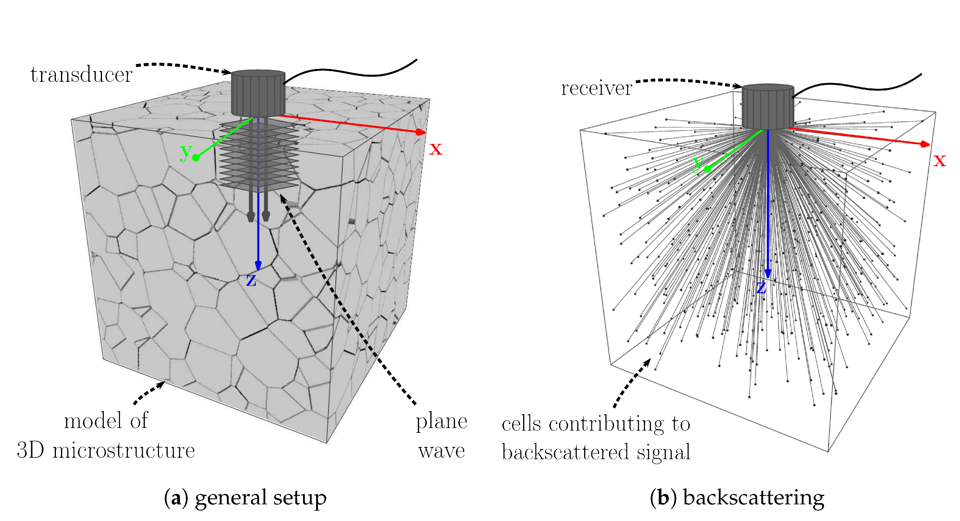
We perform a virtual ultrasonic pulse-echo-test in an explicitly given 3D microstructure generated by a stochastic microstructure model as sketched in Figure 1. The microstructure model’s parameters are determined by fitting to the grain size distribution observed in images. Using the found model parameters, we generate representative realizations of the model. In these 3D microstructures, we finally simulate numerically the ultrasonic testing by the pulse-echo-technique as sketched in Figure 1. We do not simulate the back wall response. Instead, we compute the backscattered contribution from the entire microstructure for each realization of the model. We superpose the response signals in frequency domain yielding a spectrum. Finally, we apply the Fourier transform resulting in a time-domain signal. Altogether, a set of 3D microstructures leads to a corresponding set of time-domain signals.
This paper devises a method for computing ultrasonic microstructural noise based on a geometric model of the investigated polycrystalline material. More precisely, we simulate scattering due to individual grains. Note that this is not the same as the so-called grain noise well-known from ultrasonic experiments. The difference is due to the virtual experiment being still much simpler than the real one as it does not capture at all multiple scattering—a non-negligible source of microstructural noise in real ultrasonic experiments.
We compute the wave propagation for two microstructures, i.e., Inconel-617 and titanium, with strongly varying properties, see Table 1. ASTM classifies microstructures by average grain diameters observed in 2D micrographs [30]. According to this classification, Inconel-617 is class no. 2 (0.185 mm) and titanium class no. 8 (0.022 mm). Scattering coefficients are computed for nickel, too, to compare with [13,31]. Due to lack of microstructure data, we do not fit a model but calculate the spatial scattering function based on the effective diameter from [13,31], only.
We model the propagating wave as a planar one, as indicated in Figure 1. That is, the wave is constant in a plane perpendicular to the propagation direction.
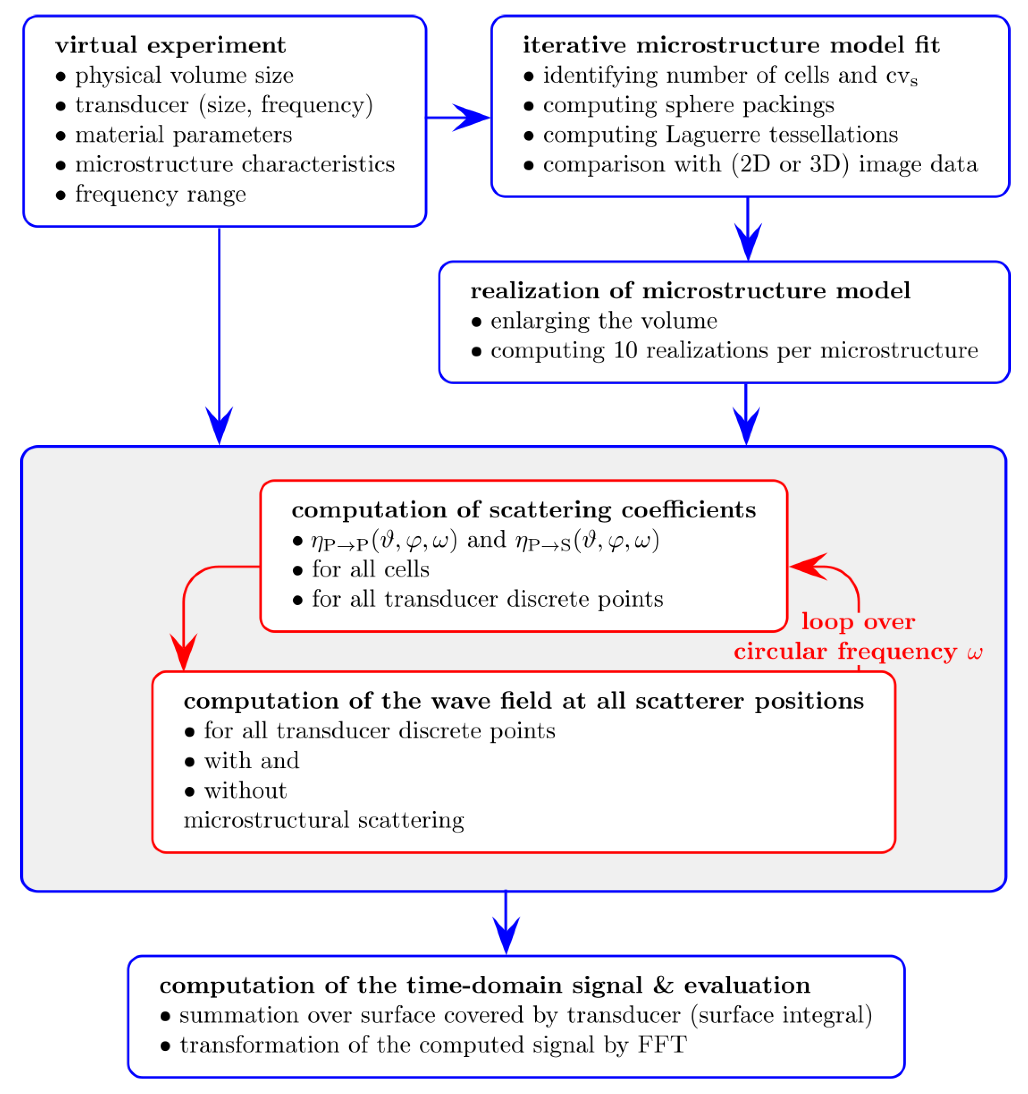
Our workflow is sketched in Figure 2. There are three steps to be taken: First, the transducer as well as the transducer’s bandwidth are discretized according to the sampling theorem [34]. The required parameters are listed in the upper left box of Figure 2. Also in the first step, the microstructure model is fitted and representative realizations are generated, see the right upper boxes. In the second step, the displacement field at scatterers’ positions due to wave propagation in momentum space is computed. Finally, in the third step, we transform the signal into the time domain using the Fast Fourier Transformation. Note that the scheme in Figure 2 is already specialized to modelling the microstructure by Laguerre tessellations generated by random packings of hard spheres.

2.1. Scattering Theory

The ensemble average of a physical quantity is the mean of this quantity over a state of the considered system [35,36] with the region or time interval of averaging being comparable to the slot when or where the observed system changes its state. Scattering effects due to local microstructural inhomogeneities vary with grain size and orientation, and thus have to be captured at the scale of the grains. The scattered energy densities for a certain volume of a particular medium can be derived from the microscopic position dependent material characteristics like single crystal elastic constants and density and the ensemble average.
Ensemble averaging for ultrasonic propagation in polycrystalline materials has been used for a long time, see e.g., [37,38,39]. Here, we follow the idea of Hirsekorn [13,40] and investigate the effects of closely packed scatterers. In [13], the elastodynamic equation of motion is solved assuming small deviations due to microstructural variation. This variation is captured by modelling the microstructure as a system of closely packed scatterers exposed to the propagating ultrasonic wave. The scattered energy flux relates the frequency dependent time harmonic displacement field for one vibrating cycle and the material specific stress tensor, see [7] for more details.
The Born series [41] for the propagating wave yields an approximation of the resulting displacement field. Material dependent parameters like size and orientation distribution of the grains are accounted for by the geometric correlation function. Ensemble averaging is applied to the Born series terms. Finally, the energy flux is derived as an infinite sum, time averaged over one vibration cycle. The n-th order Born approximation of energy flux is the corresponding n-th partial sum, n = 0 , 1 , . It represents the incident and scattered waves’ interaction with the microscopic inhomogeneity of the material. Hirsekorn uses the lowest non-zero order Born approximation to derive an analytical expression of the ensemble averaged total energy flux due to scattering waves for both, incoming and outgoing waves [13]. Thus, using this approach, only first-order scattering events are taken into account, no multiple scattering. The sum of outgoing and incoming waves equals zero due to the conservation of energy [13]. Here, we consider the outgoing waves, only, as we aim at revealing the backscattered wave contributions.

2.1.1. Geometric Correlation Function

Ensemble averaging in polycrystals incorporates microstructural features by multiple-point correlation functions of the local crystal orientations. In order to be feasible, approximations use a variety of simplifications, e.g., only 2-point or pair-correlations. If the orientations of grains are assumed to be independently distributed, then the 2-point orientation correlation boils down to the orientation distribution function multiplied by the geometric 2-point correlation—the probability of two points falling into the same grain [42,43]. The latter depends exclusively on the distance of the considered points if the structure is macroscopically homogeneous and isotropic.
Stanke and Kino [8] incorporate the 2-point correlation function W ( r ) into their unified theory of elastic wave propagation assuming it to decline exponentially: W ( r ) = exp r / ¯ , where r is the distance of a point pair and ¯ is the mean chord length of the grains, also called mean free path length or correlation distance. This simple shape of the orientation correlation is convenient yet not realistic, see [44,45] and references therein. Following [8], Hirsekorn [13,40] derives from ¯ the effective volume V eff of a scatterer as
V eff = ψ = 0 π θ = 0 2 π r = 0 exp r ¯ d r d θ d ψ = 8 π ¯ 3 .
Roughly speaking, V eff can be interpreted as the volume that scatters if the correlation length is ¯ . Plugging in V eff into the Born approximation yields the scattering coefficients reported in [13].
We aim at emphasizing the contribution of individual grains to microstructural noise. Thus, we follow [13,40] in treating the grains as homogeneous and completely independent scatterers. However, we observe the effective scatterers’ volumes V eff directly as the cell volumes in our tessellation model realizations. The effective diameter d eff of a cell or grain is derived as the diameter of the sphere of volume V eff
d eff = 6 / π V eff 1 / 3 .

2.1.2. Spatial Scattering Function

Evaluating the second order term of the Born approximation and utilizing Equation (1) yields analytical representation of scattering coefficients η ϑ , φ , ω with ω = 2 π f being the corresponding circular frequency and f a fixed frequency. ( ϑ , φ ) 0 , π × π , π are the spherical polar coordinates of the local coordinate system, whereat η ϑ , φ , ω maps the scattering coefficients along spatial directions around a scattering volume V eff . Thus, we call this analytical representation of scattering behavior spatial scattering function.
The following notation is used throughout: Denote by k P , k S the wave numbers for the pressure (P) and shear (S) waves, respectively. The subscript is made of incoming→outgoing wave, which is either pressure or shear, respectively. The spatial scattering functions are:
η P P ϑ , φ , ω = k P 8 d eff 3 π 6 3 4 π ϱ ω 2 2 1 1 + k P 2 ( 1 + cos ϑ ) d eff 2 2 6 3 2 A 2 cos 4 ϑ + A 1 sin 4 ϑ + 2 ( A 5 + 2 A 6 ) sin 2 ϑ cos 2 ϑ
η P S ϑ , φ , ω = k P 3 k S 5 d eff 3 π 6 3 4 π ϱ ω 2 2 1 1 + ( k P 2 + k S 2 + 2 k P k S cos ϑ ) d eff 2 4 6 3 2 A 6 ( 2 sin 2 ϑ ) + A 4 sin 2 ϑ + ( A 2 + A 1 2 A 5 4 A 6 ) sin 2 ϑ cos 2 ϑ
η S P ϑ , φ , ω = k P 5 k S 3 d eff 3 π 6 3 4 π ϱ ω 2 2 1 1 + ( k P 2 + k S 2 + 2 k P k S cos ϑ ) d eff 2 4 6 3 2 A 4 sin 4 ϑ sin 4 φ + A 6 ( sin 4 ϑ cos 4 φ + cos 4 ϑ ) + 2 ( A 9 + 2 A 10 ) sin 2 ϑ cos 2 ϑ cos 2 φ + 2 ( A 7 + 2 A 8 ) sin 2 ϑ sin 2 φ ( sin 2 ϑ cos 2 φ + cos 2 ϑ )
η S S ϑ , φ , ω = k S 8 d eff 3 π 6 3 4 π ϱ ω 2 2 1 1 + k S 2 ( 1 + cos ϑ ) d eff 2 2 6 3 2 A 8 + A 10 + ( A 8 A 10 ) sin 2 ϑ sin 2 φ + ( A 6 + A 4 2 A 7 4 A 8 ) sin 2 ϑ sin 2 φ ( sin 2 ϑ cos 2 φ + cos 2 ϑ ) + 2 ( A 6 A 9 2 A 10 ) sin 2 ϑ cos 2 ϑ cos 2 φ
with ϱ being the materials’ density. Equations (2)–(5) presume a specific incoming pressure or shear wave given by wave vector ( 0 , 0 , 1 ) T in both cases, and either the pressure polarization vector ( 0 , 0 , 1 ) T or shear polarization vector ( 1 , 0 , 0 ) T . This presumption sets up the relation between single scatterers and the transducer, which is the source of the incoming wave. As in [13,46], this models how single scatterers and the transducer interact. Here, A 1 , , A 10 denote the ensemble averaged elastic constants from [40] listed in Table 2 below.
The spatial scattering functions are defined in intrinsic coordinates, with the origin of the local coordinate system in the center of scattering volume V eff . In terms of Cartesian coordinates x 1 , x 2 , x 3 T = r sin ϑ cos φ , sin ϑ sin φ , cos ϑ T , the positive x 3 -axis of the local coordinate system is aligned with the positive z-axis of the global coordinate system. 
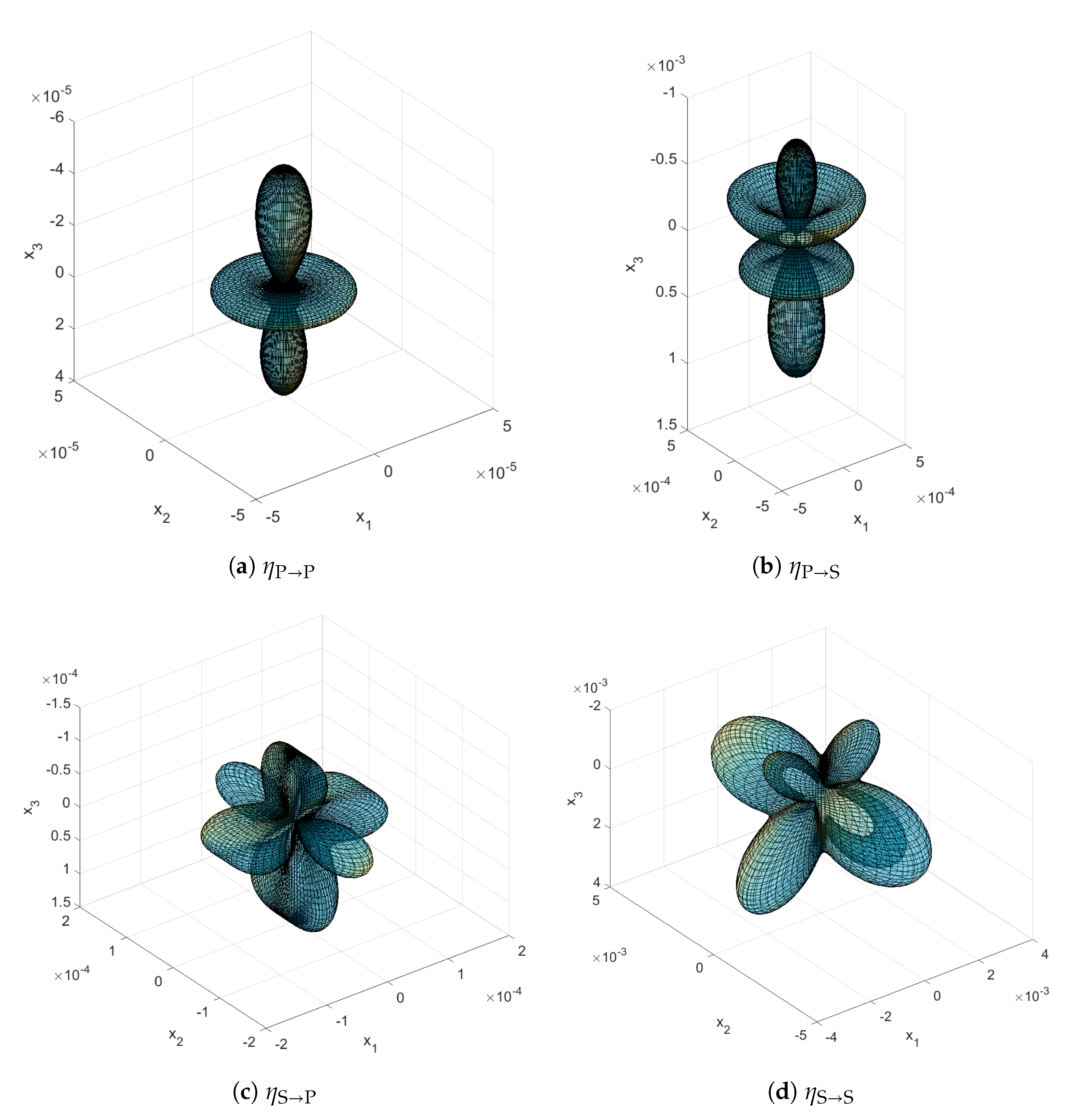
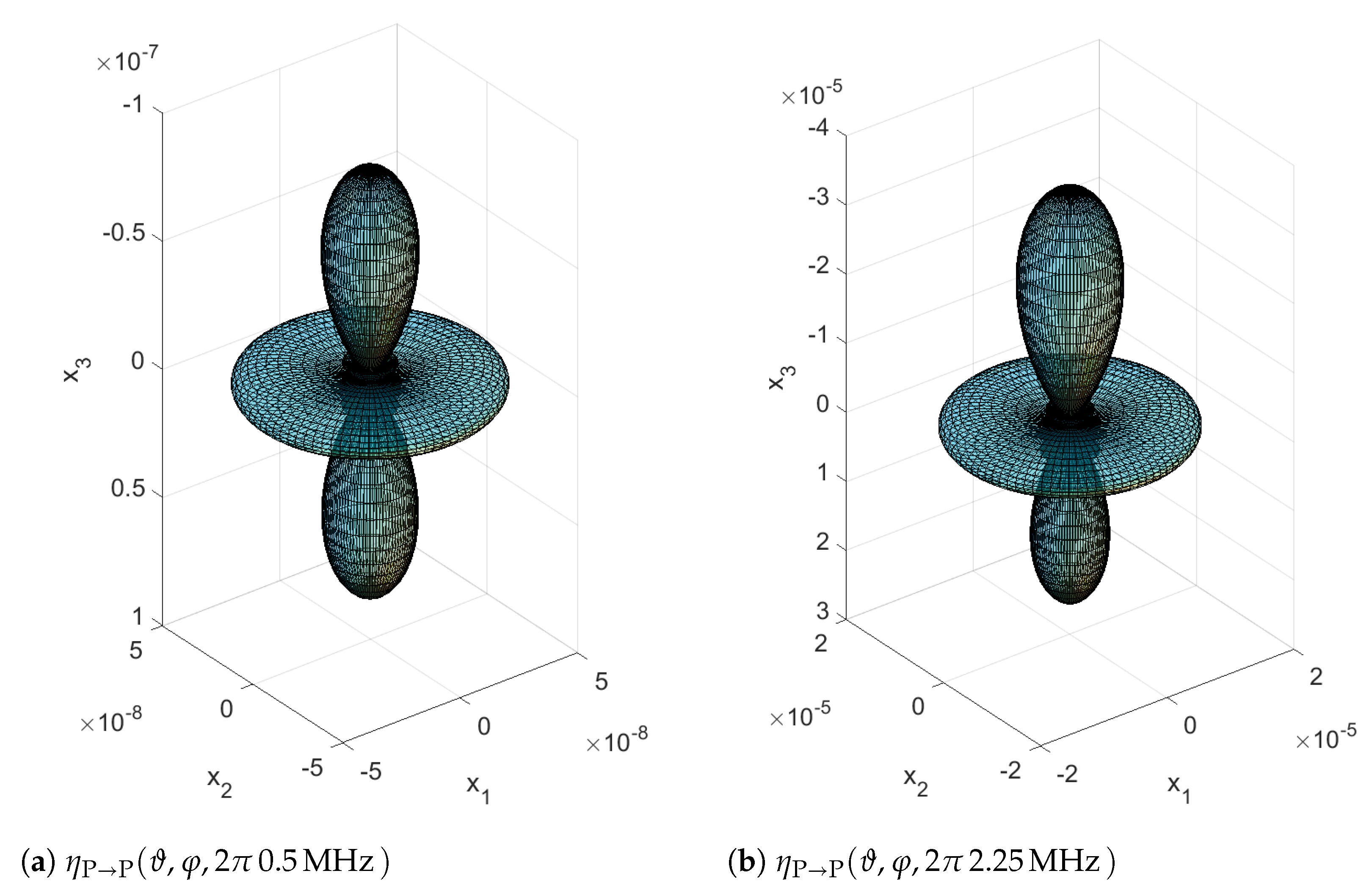
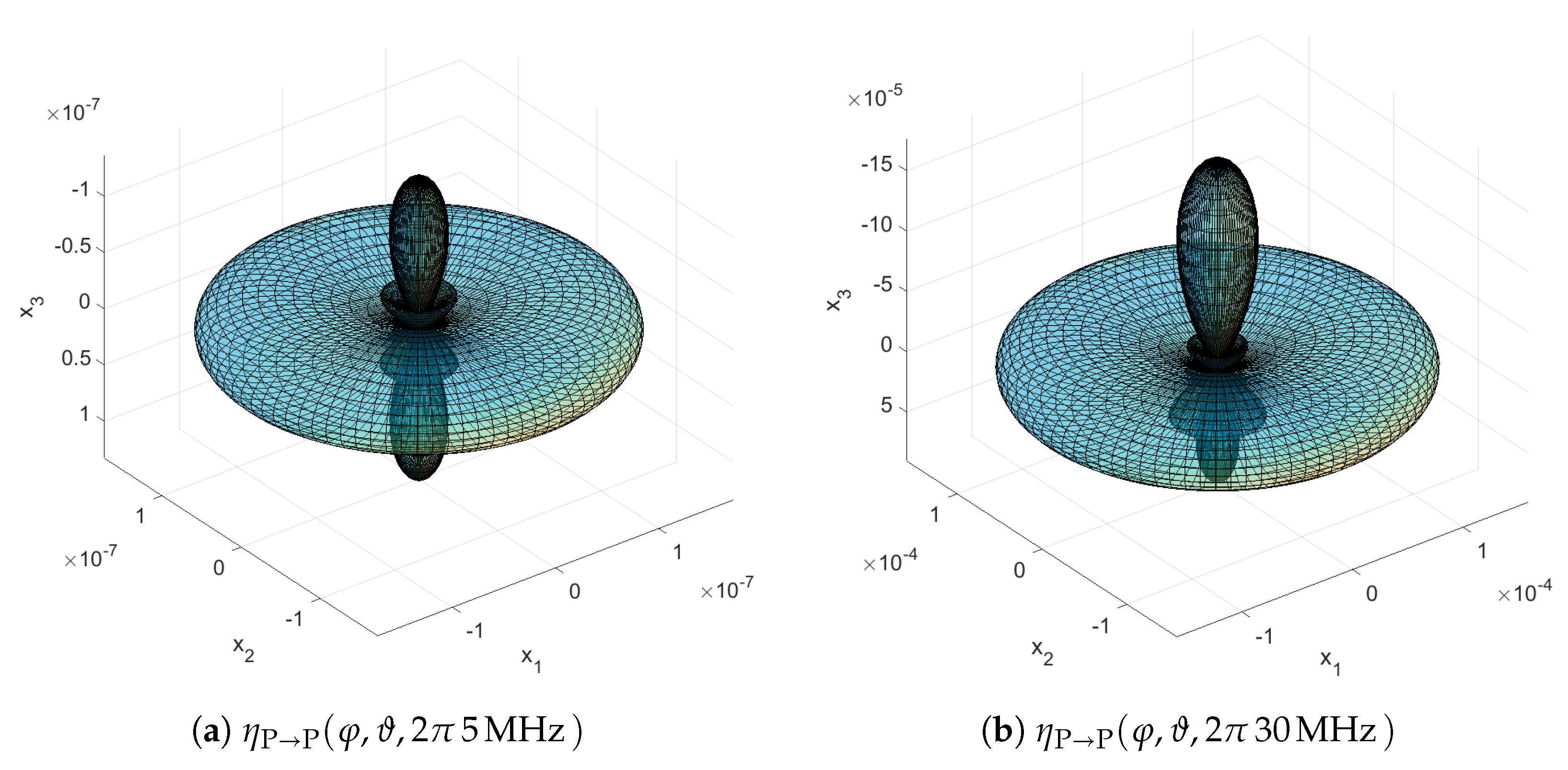
Figure 3 shows the spatial scattering function for a single scatterer in nickel (see also Table 1). In the following, we use Cartesian coordinates and the base unit mm 1 in all graphical representations of the spatial scattering functions.
In [13], the normalized scattered wave coming from a point in the material is plotted in two dimensions, in [31] the same is done for the normalized scattered wave coming into a scatterer. These quantities depend however on all three spatial directions. We therefore visualize the normalized scattered wave coming from a scatterer from [13] in three dimensions.
To summarize, we model each grain as a cell contributing by its volume V eff to the backscattered ultrasonic signal. The cell’s orientation is accounted for by the ensemble averaging. The Born approximation relies on a macroscopic isotropy of the microstructure. That means, in all further steps, cells do not have a specific orientation anymore. Note however, that our workflow in principle carries over to modelling the orientation and its scattering effect, too.

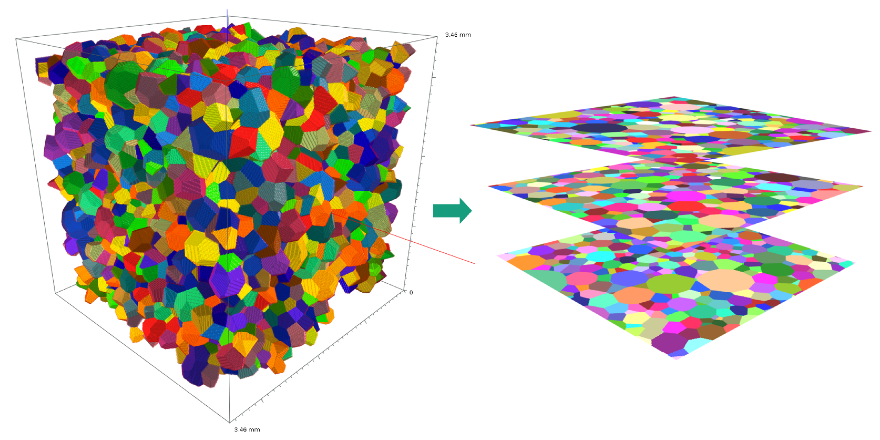
2.2. Geometric Modelling of Polycrystalline Microstructures

There is a wide variety of geometric characteristics describing spatial size and shape of grain systems. A basic and in some sense complete system of characteristics for the grains are the intrinsic volumes or Minkowski functionals [47]. Ohser’s algorithm allows to estimate them efficiently based on 3D image data [
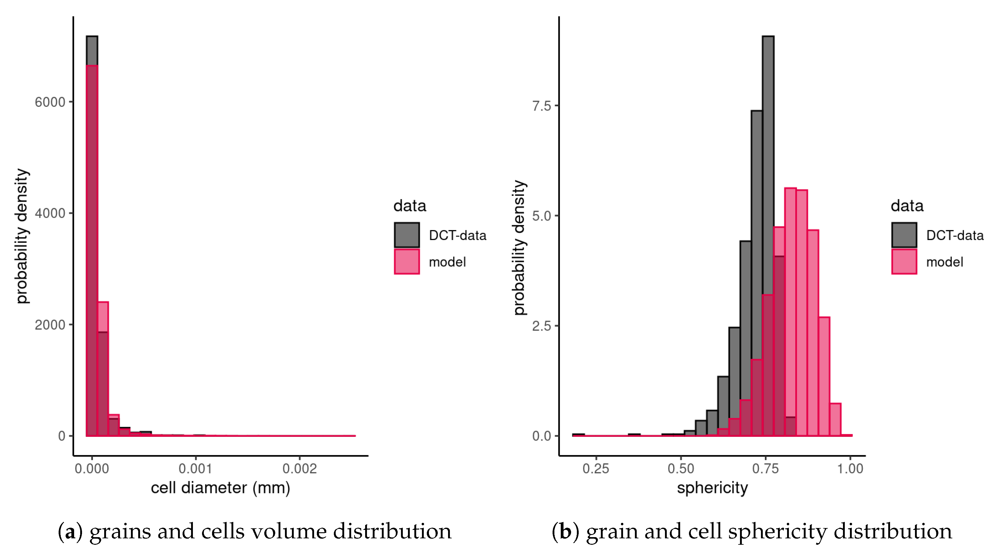
48]. For the titanium, we use the volume V, and the isoperimetric shape factor
s = 6 π V / S 3 / 2
derived from volume and surface area S. This dimensionless index, often called sphericity, is normalized such that it attains the value 1 for a perfect sphere. Moreover, 0 s 1 with 1 being reached by the sphere, only.
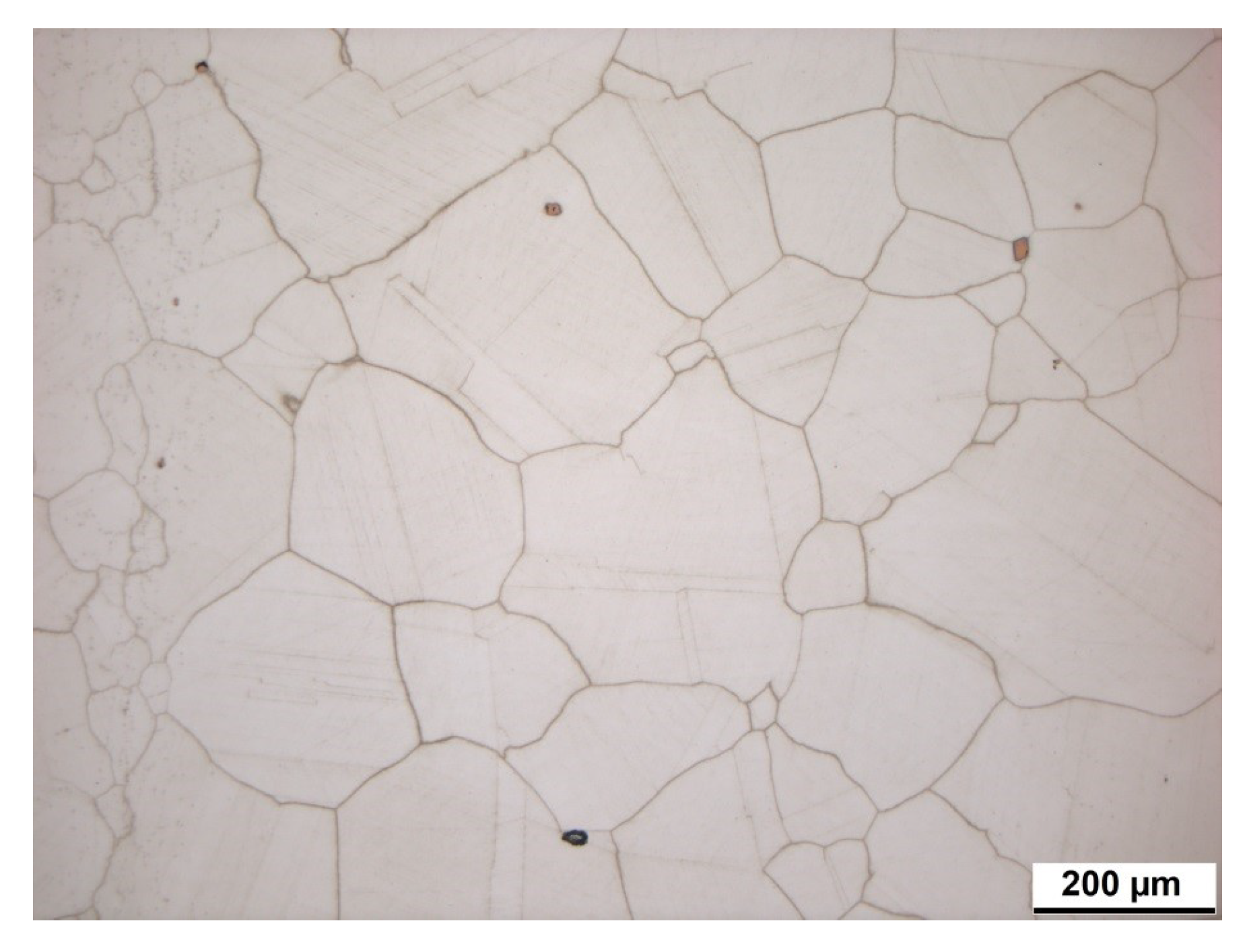
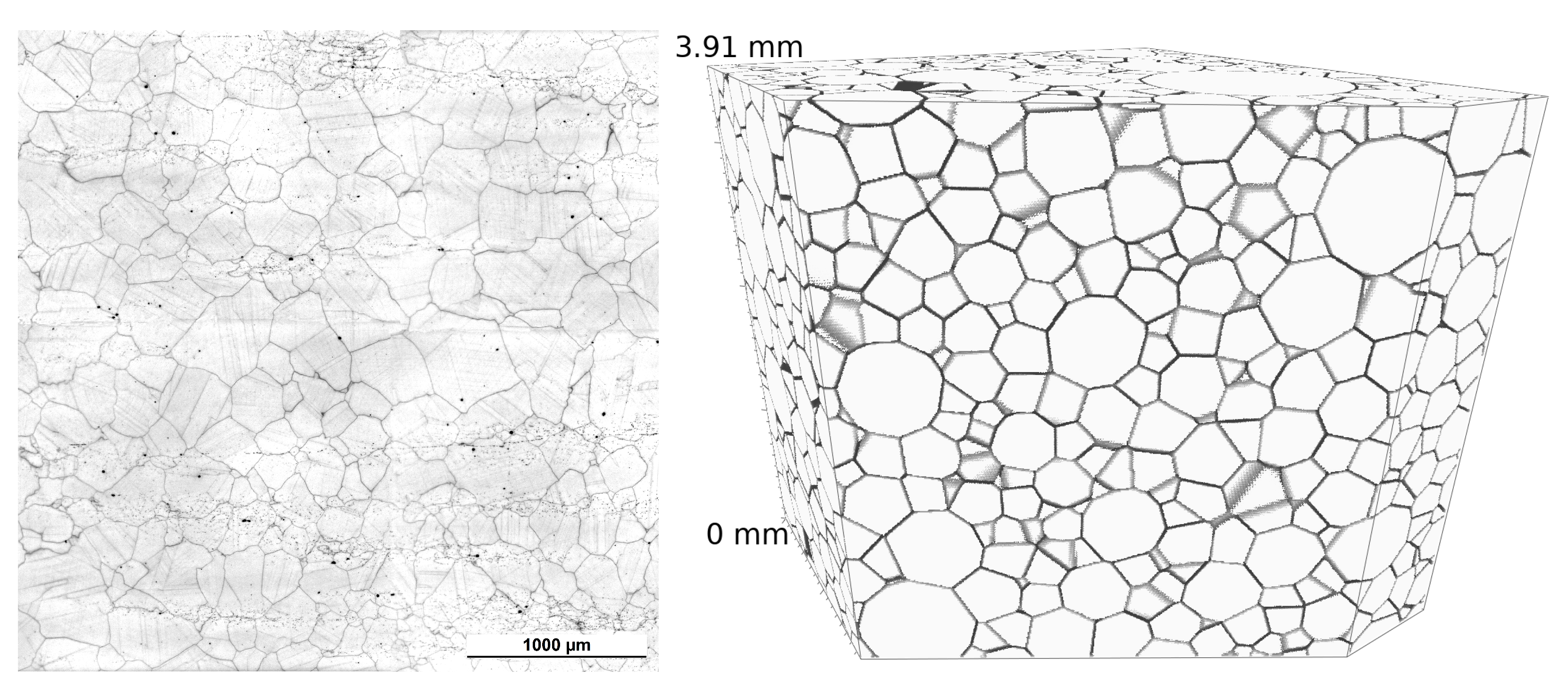
For the Inconel-617, we use the maximal Feret or caliper diameter of the 2D grain cross sections—basically the longest Euclidean distance of two points in that grain.

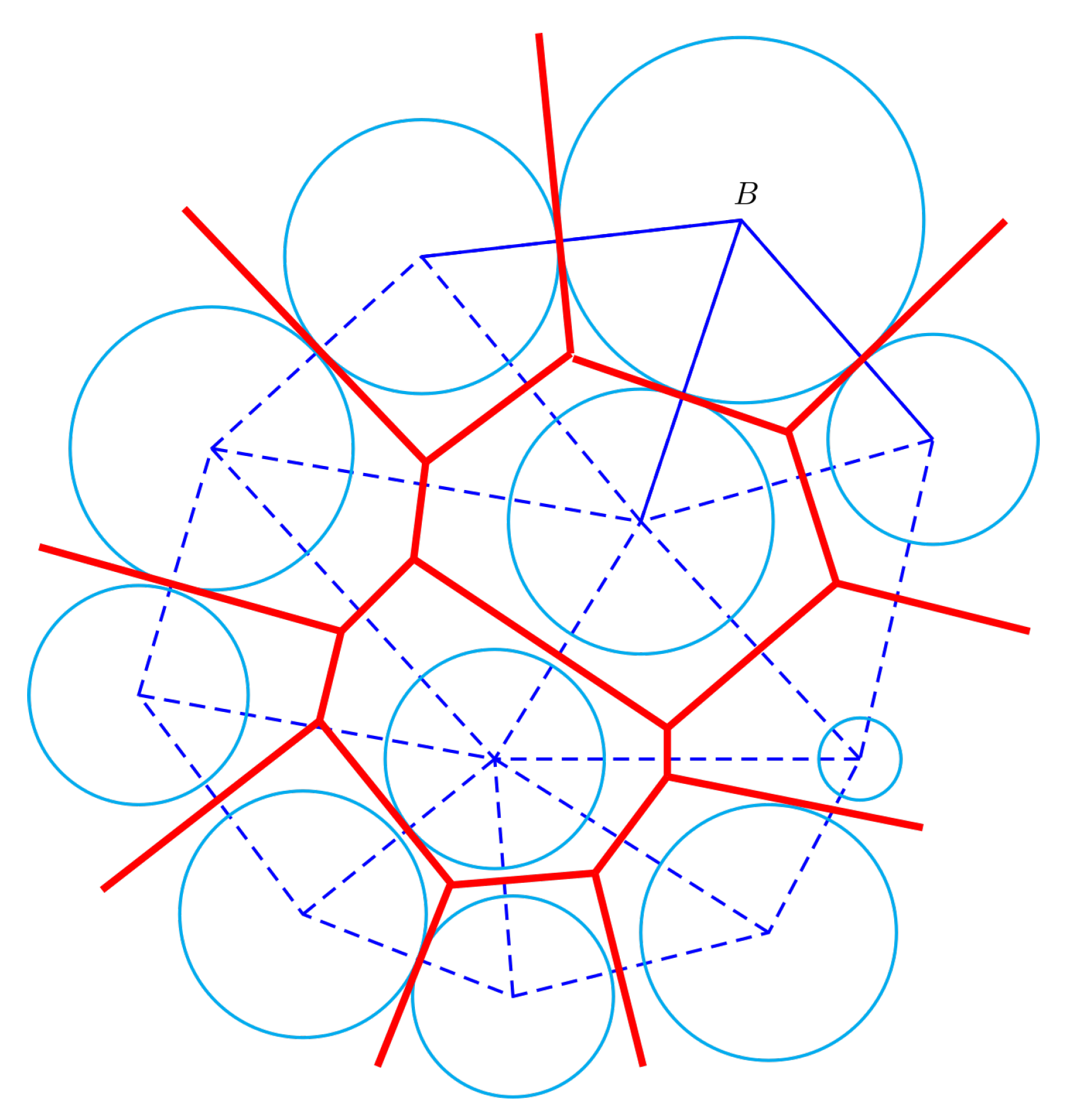
2.2.1. Laguerre Tessellations

Random tessellation models are used to model the grain structure of polycrystalline materials in many contexts [20,21,49,50]. Most common are Voronoi tessellations, dividing space by assigning each point to the nearest generator. In Laguerre tessellations, this well-known rule is generalized such that generator’s attraction is steered by an additional weight [51]. The thus achieved higher flexibility allows for better control over cell sizes, see Figure 4. Laguerre tessellations generated by random closed packings of spheres are a standard model for rigid foams [52,53,54,55] and popular models for polycrystals [5]. Methods for fitting in the statistical sense [52], reconstruction from 2D images [56] or cell centroids and volumes in 3D [21], as well as approximation based on 3D image data [20] are available.
Here, we use Laguerre tessellations generated by random packings of spheres. We use the force biased collective rearrangement algorithm [57], an effective modification of [58] in the way described by [59,60]. This choice is motivated by the good control over the cell volume distribution this model allows. Note that Fan [5] builds on a collective rearrangement packing, too [61,62].
For the sake of independence, we sketch the mechanism of the force biased packing algorithm: At the beginning of the packing, spheres with an outer soft shell and an inner hard core are placed in the container. The shells are allowed to overlap. Spheres push each other away with forces depending on the overlap. In a collective rearrangement step, they move according to the cumulative forces of repulsion. Then, the outer shells of the spheres decrease while the cores grow up to the size that just prevents overlap of the cores. These steps are iterated. The packing ends if the desired packing density—proportion of the volumes of the sphere system and the container—is reached or the shells have disappeared or the number of iterations has reached a predefined limit. See 
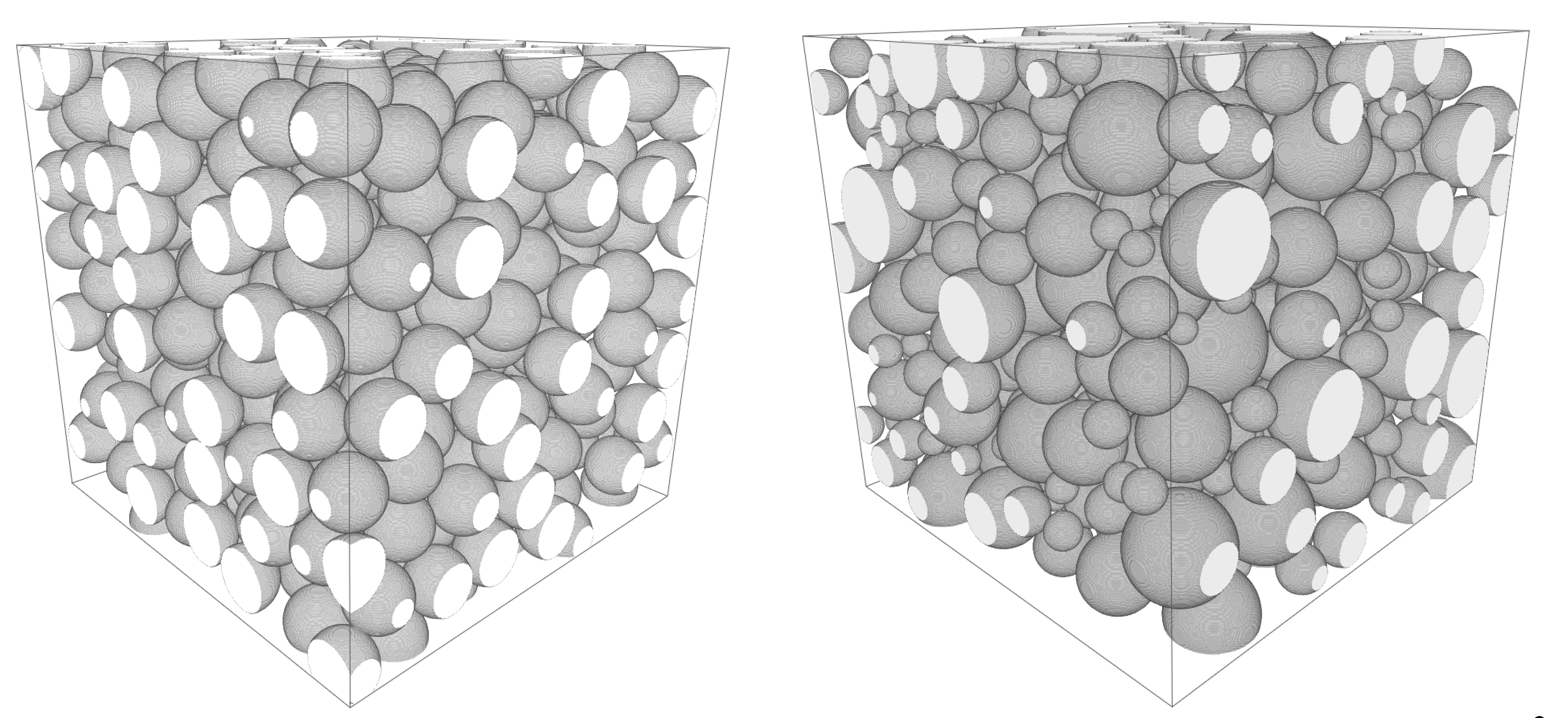
Figure 5 for the volume rendering of a thus derived sphere system.
The cell structure modeling the polycrystal is then derived from the sphere packing by the Laguerre mechanism: We denote by x i R 3 the center and by r i R the radius of sphere i for i = 1 N C . Then ( x i , r i ) i = 1 N C is a set of generators with non-negative weights. A point y R 3 is assigned to the cell C ( x i , r i ) generated by x i if its weighted distance to x i is smaller than to any other generator. The point y is assigned to the i-th cell if x i y 2 r i 2 is less than x j y 2 r j 2 for all j i . The wall between two neighboring generators is the perpendicular bisector between their respective spheres, see Figure 4 for an illustration of the mechanism.
That way, our random system of non-overlapping spheres divides the space into convex cells C ( x i , r i ) with diameters d eff , i of volume equivalent sphere as given by (1). Additionally, we equip each cell with its center of mass m i .

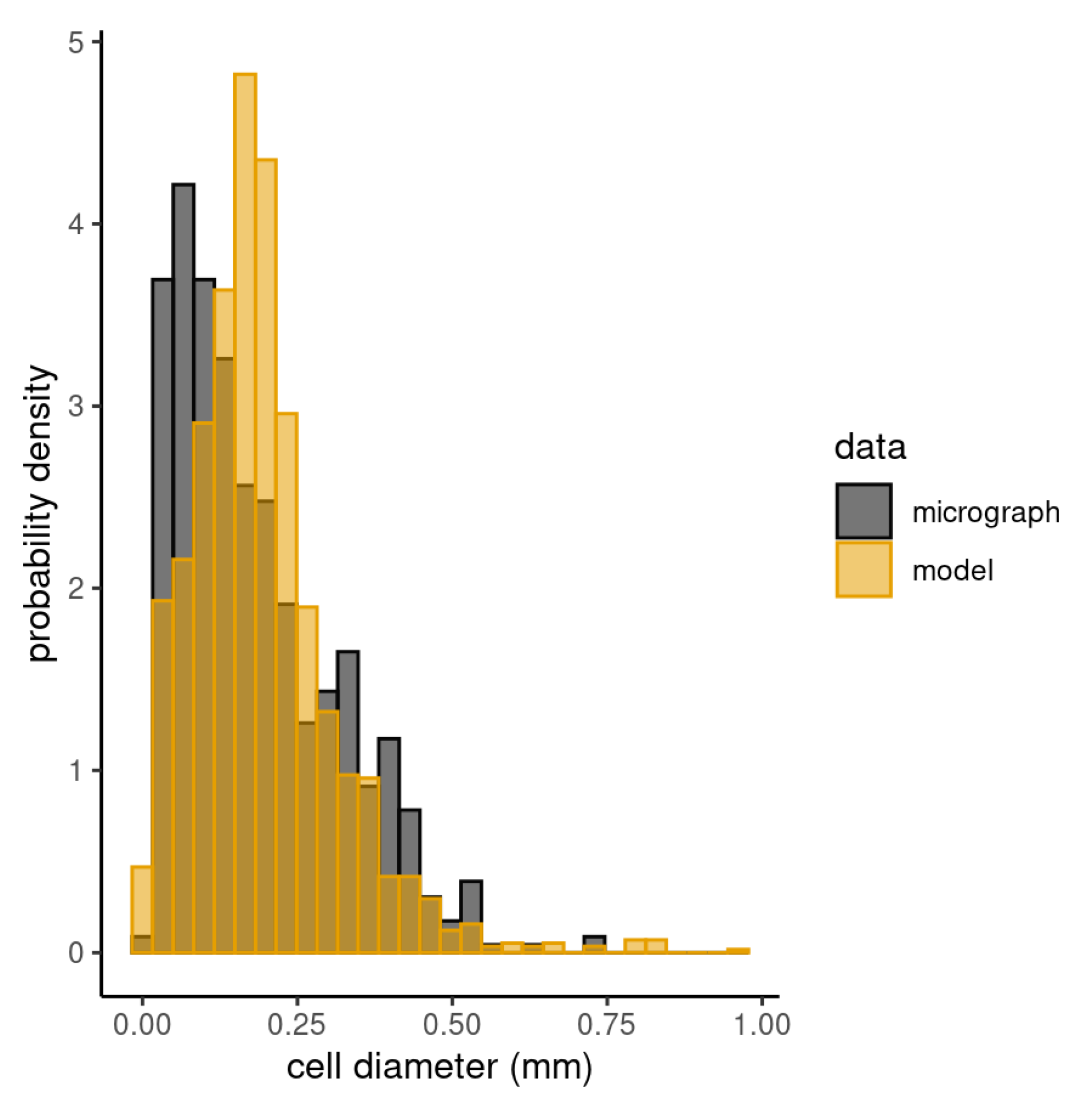
2.2.2. Grain Size Distribution

Grain sizes in polycrystalline materials are usually assumed to be log-normally distributed [4,63]. In Laguerre tessellations generated by dense sphere packings, the cell size distribution is dominated by the size distribution of the generating spheres [5,52]. We therefore model the sphere volumes v s according to a log-normal distribution. The probability density function h of the log-normal distribution with parameters ( μ , σ ) is:
h v s | μ , σ = 1 v s σ 2 π exp ( ln v s μ ) 2 2 σ 2 .
Expected sphere volume v ¯ s = V V / N V and the sphere volume standard deviation σ v s are then [52]
v ¯ s = exp ( μ + σ 2 / 2 ) ,
σ v s = ( exp ( σ 2 ) 1 ) exp ( 2 μ + σ 2 ) .
On the other hand
μ = 1 2 log V ¯ 2 / ( cv s 2 + 1 ) ,
σ = log ( cv s 2 + 1 )
with cv s = σ v s / V ¯ denoting the coefficient of variation of the sphere volume.
Note that the coefficients of variation of the resulting grain volumes cv g and the generating spheres cv s surely differ with cv g > cv s . For very dense sphere packings as in [5], the difference is small as the cells do not differ strongly from their generating sphere. If the sphere packing density V V is lower, the difference grows. We use the cubic polynomial in cv s fit to cv g for the densely packed case from [5]. See [52] for a more general discussion.

2.2.3. Fitting the Geometric Model Based on 2D Image Data

Model fitting solely based on 2D image data is an ill-posed problem. In [56] an optimization based on a goodness-of-fit criterion for 2D slices is devised to avoid costly simulations of the full 3D Laguerre tessellations. However, [56] aims at exact reproduction of the observed 2D cell structure. Here, we can use a simpler approach, closer to [50]: We simulate 3D tessellations, compare 2D slices cut from them with our 2D observations, and alter the parameters to reduce the differences. This is repeated till the fit is sufficiently good.
First, we estimate the expected number of grains per volume N V . There is no straight forward method to do so based on the observed grain number in planar sections N A in case of Laguerre tessellations generated by sphere packings. However, for the special case of a spatial Voronoi tessellation generated by a Poisson point process [47] (10.74) yields:
N A = 1.46 N V 2 / 3 .
Following the recommendation from [47] to use this approximation for the non-Poisson case, too, we set the initial number of cells to the value which is expected for the Poisson Voronoi tessellation case. The initial guess for the coefficient of variation of the sphere volume distribution is set to 1.5 as this is about the center of the range cv g [ 1.09 , 2.13 ] for the grain volumes reported by [5].
We generate a force biased sphere packing using mean sphere volume V V / N V and cv s = 1.5 , derive the Laguerre tessellation, extract planar sections, and compare them with the 2D micrographs based on the Feret diameters of the cells. We adjust the number of spheres in the random packing based on comparison of the maximal Feret diameters and iterate till the mean maximal Feret diameter (or the cell density) is met.
In the second step, the coefficient of variation of the sphere volumes cv s is fit by a simple grid search. Again, we compute sphere packings and derive the corresponding Laguerre tessellations. We take five section planes in each of the three coordinate directions, measure the maximal Feret diameters, and compare the mean maximal Feret diameter and the standard deviation of the maximal Feret diameters in these 2D sections with the corresponding characteristics measured in the 2D micrographs. We finally choose the value for cv s yielding the best agreement.

2.3. Simulation of Wave Propagation

We simulate the wave propagation in momentum space by calculating displacement at scatterers’ positions, as drafted in Figure 1. First, we compute the displacement induced by a propagating wave. We discretize the surface covered by the transducer by N t source points y k R 3 , k = 1 , , N t . After all, we evaluate the energy contribution along these particular spatial directions, i.e., m y . Here, u I R 3 is the incoming polarization vector and c I R the group velocity, both determined by vectors y and m. The displacement u α R 3 due to propagation of an elastic plane wave can be modelled at scatterers’ positions as a superposition of all source points by
u α m , ω = U I 4 π k = 1 N t u I exp ( j ω m y k ) / c I m y k
with α indicating incoming pressure (P) or shear (S) waves, j the complex unity and U I denoting the amplitude of the propagating wave.
The second contribution is the displacement due to scattering at scatterers’ position. We define the latter following Equation (8) in [64], namely:
u α , sc m , ω = U I 4 π exp ( j ω m y ) / c I m y u I + R S u S R + R P u P R
with R S and R P being the reflection coefficients. Thereby, all polarization vectors contribute to the result—those of the incoming (I) as well as those of the reflected (R) waves. We adapt Equation (13) by replacing the reflection coefficients by the scattering coefficients given analytically in Section 2.1.2. This yields
u α , sc m , ω = U I 4 π k = 1 N t exp ( j ω m y k ) / c I m y k u I + η α S ( ϑ k , φ k , ω ) u S R + η α P ϑ k , φ k , ω u P R .
The polarization vectors u α R R 3 of the reflected contributions are evaluated in direction of the corresponding slowness vectors. Červený [65] defines the reflected slowness vector as a function of incoming slowness vector and thus the reflected contributions are governed by the corresponding slowness vectors i.e., s α R m y . Also, the direction of reflected slowness vectors governs the scattering coefficients. The scattering coefficients in Equations (2)–(5) are derived as
ϑ k = arctan s y ( m y k ) s x ( m y k ) φ k = arctan s z ( m y k ) s x 2 ( m y k ) + s y 2 ( m y k )
where the subscripts x , y , z represent the components of s α R . In Equation (14), the angle and frequency specific scattering coefficients depend on the single crystal parameters, but the group velocity c I on the polycrystal’s material parameters.

2.3.1. Reciprocity Relations

We follow [66] in applying the reciprocity relations for computing the displacement at the receiver’s surface. In [66], a formalism for scattering of ultrasonic waves at scatterers is derived, in particular for the Born approximation. There, the received signal is defined as the integral over the scatterer’s entire surface. Here, the displacement at the receiver is expressed by the superposition of displacement velocity j ω u and stress tensor σ ̲ ̲ at all scatterers’ positions m i :
u ω = j ω 4 i = 1 N C u α , sc m i , ω σ ̲ ̲ u α m i , ω σ ̲ ̲ α , sc · n ^ ,
where n ^ R 3 is the normal to the scatterer’ surface. Note that, although we account for one discrete point per scatterer, only, this scatterer is nevertheless assumed to be spherical. Thus, the point first reached by the wave is the one with surface normal pointing towards the transducer. Usually, transmitter and receiver are differentiated [66,67]. In our setting of a pulse-echo experiment, the transmitter however equals the receiver.

2.3.2. Modelling of the Bandwidth

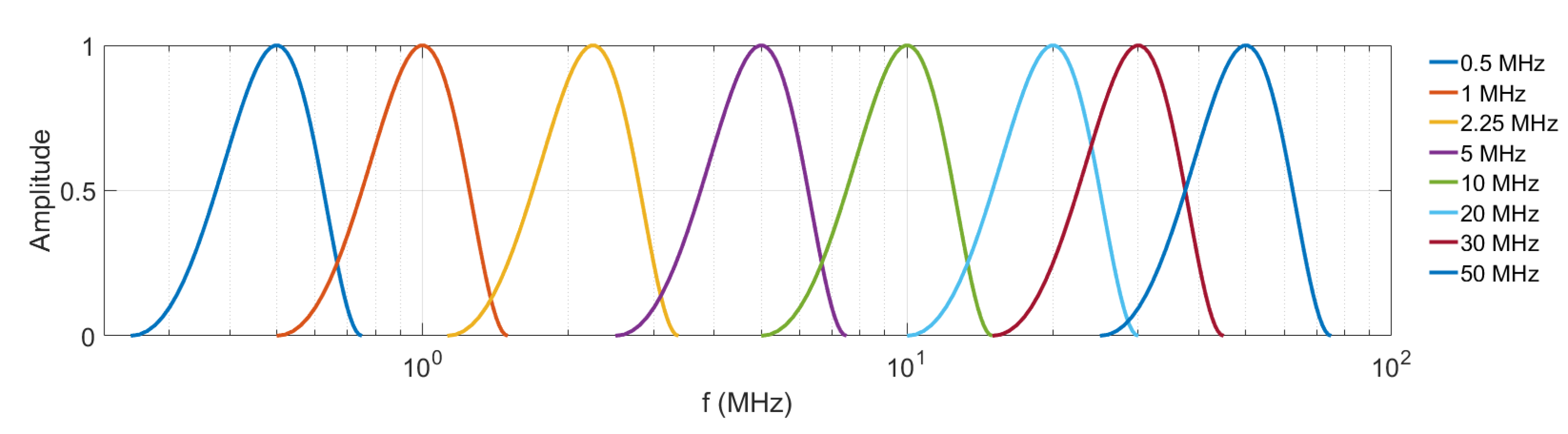
In general, wave propagation is a time-dependent phenomenon. In [68], transient signals are computed based on the static continuous wave displacement method. We model the bandwidth f m by
f m = sin 2 π f f l f r f l , f l < f < f r 0 , else .
Basically, we assume a transducer with a mid-band frequency f = 2 π ω and model f m . This yields the transducer specific harmonic displacement field in Equation (15) for a bandwidth f l < f < f r . 
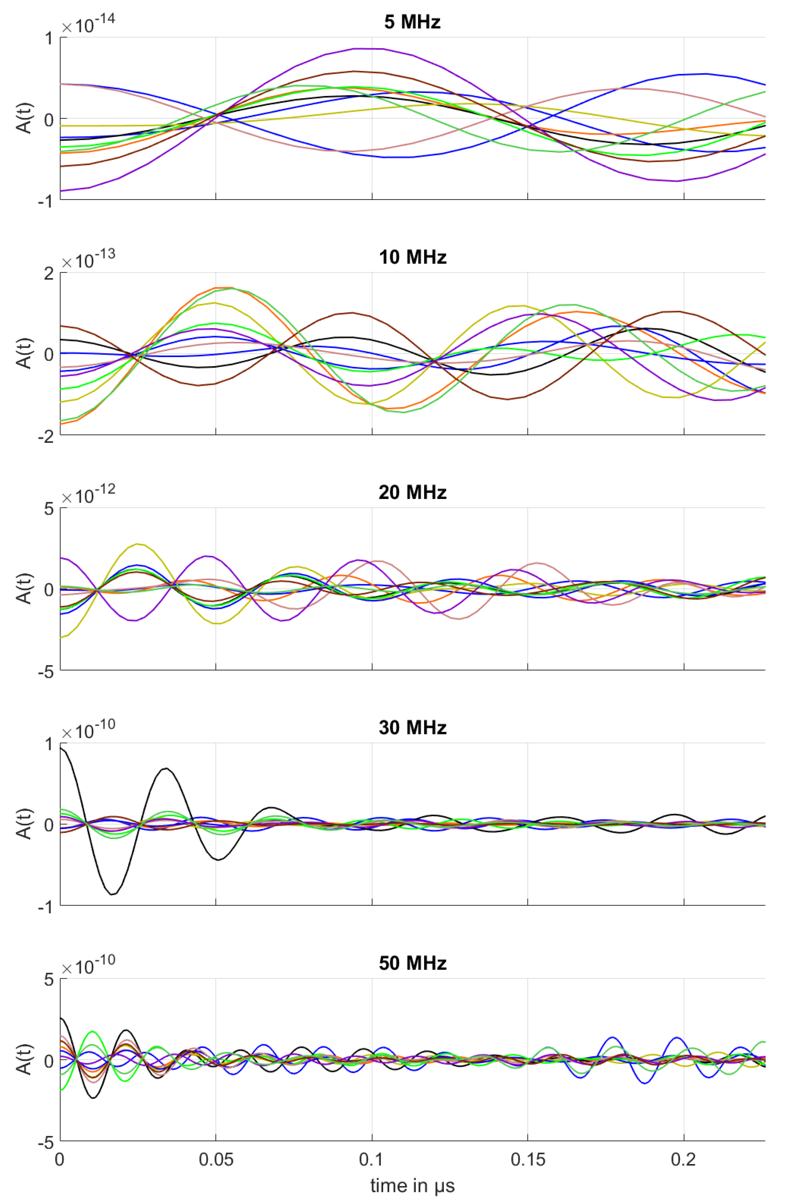
Figure 6 shows the variety of frequencies we use in the following virtual experiments.
In the virtual experiments, we assume the ultrasonic transducer in pulse-echo technique emitting and receiving pressure wave, which mimics varying mid-band frequencies. Finally, we transform the result into the time domain by MATLAB’s inverse Fast Fourier Transform (FFT) [69,70].

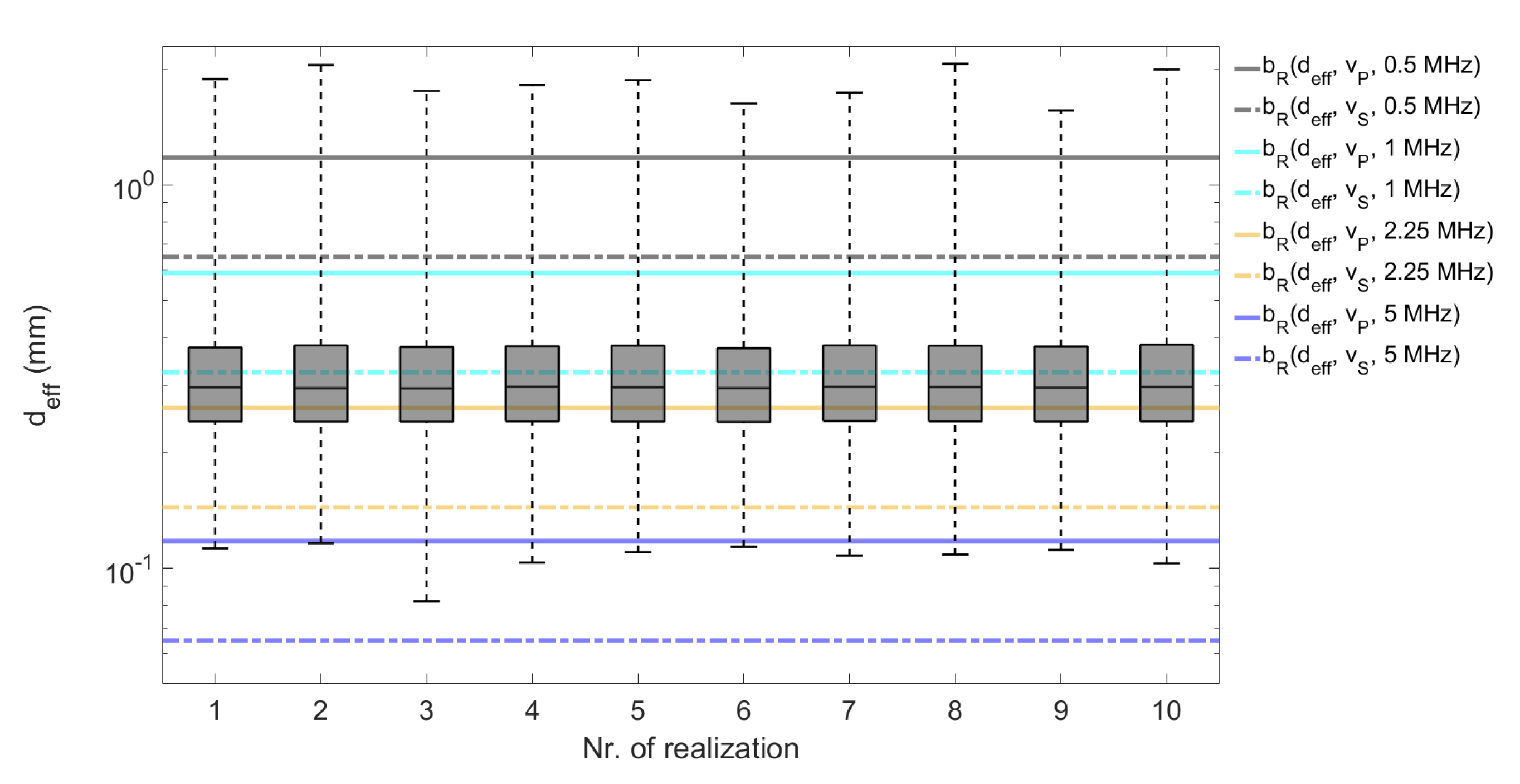
2.3.3. Evaluation Tools

A microstructure model fit yields a predefined number of microstructure realizations (cell systems) [5,52]. We aim at simulating ultrasonic specifics in these cell systems, as scattering. In ultrasonic testing, scattering regimes are roughly characterized in terms of the testing frequency f, the material dependent wave propagation velocity v α , and the effective scatterer diameter d eff , as follows [8]:
  • the low-frequency Rayleigh regime π f v α d eff 1 ,
  • the stochastic regime π f v α d eff 1 and
  • the high-frequency geometric limit π f v α d eff > 1 .
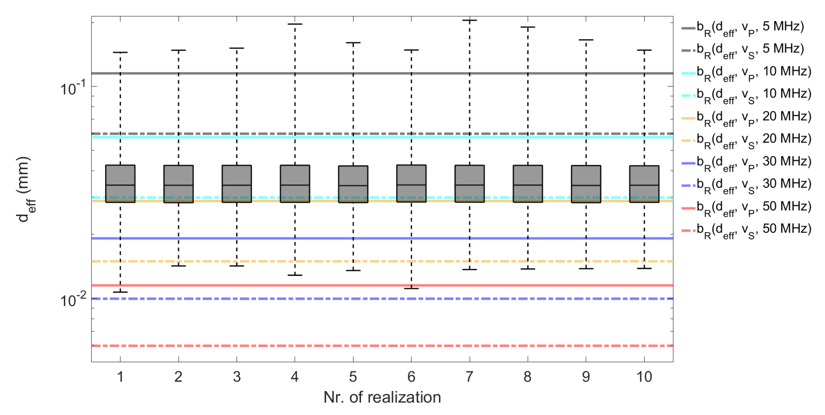
We use the Born approximation to compute backscattered wave contributions, valid in the low-frequency Rayleigh regime [13]. Accordingly, we set an upper fixed boundary for the Rayleigh regime at 0.3, which yields
d eff = 0.3 v α π f .
By this, we assume that scatterers’ size remains within the Rayleigh regime and the modeled scattering contributions are reasonable. Equation (16) corresponds to the hypothetical boundary below which the cell’s diameter stays in the Rayleigh scattering regime. We denote this boundary by b R and check whether the microstructure realizations observe this boundary.

3. Materials

We calculate the microstructural scattering for two metals—Inconel-617 and titanium. The first is represented by 2D micrographs, only, whereas for the latter three-dimensional diffraction computed tomography (DCT) data is available. The Inconel-617 alloy features coarse grains with average 2D diameter 185 µm whereas the titanium’s microstructure is much finer with just 33 µm. We extract random 2D slices along all three spatial directions from the DCT data and compute the average of observed grain 2D diameters for this particular comparison.

3.1. Computation Environment

First, we describe the environment used for the computations. According to the workflow sketched in Figure 2, we choose the number of realizations of the stochastic microstructure model. These can be generated in parallel. The tessellations are generated on a machine with eight CPUs and 16 GB RAM.
The computation of the wave fields with and without microstructural scattering, is the most time consuming step due to the high testing frequencies. These induce very fine discretizations of the transducer surface and of the frequency bandwidth of the transducer. Small grains increase the number of cells per considered volume and thus increase the computation time, too.
The loop has to be traversed three times in order to cover all dependencies: The backscattering contributions for each frequency step (bandwidth), each of the spatially arranged scatterers, and all discretization points of the transducer. For these steps, in particular the ω -loop (red box in Figure 2), a C++ parallelization using openmp [71,72] is executed on nodes with 16 CPUs and 60 GB RAM of Fraunhofer ITWM’s linux cluster [73].

3.2. Inconel-617

Inconel is the trade name for a group of nickel-chromium alloys with exceptional strength, metallurgical stability, and oxidation resistance at high temperatures [74]. Inconel alloys are therefore used e. g. in aerospace solutions, in gas turbines for combustion cans, as well as for petrochemical processing and heat-treatment equipment. Here, we analyze a macroscopically homogeneous sample of this alloy and treat its microstructure as a single phase. Microstructural information is provided by a stack of micrographs featuring bright grains separated by dark grain boundaries, see Figure 7.
Based on these micrographs, the maximal Feret diameters of the cells were determined, only, due to the notorious cell boundary reconstruction problem. In [32], isotropy of the microstructure is deduced from the analysis of micrographs from three pairwise orthogonal cutting planes. We observe altogether 666 cells in 64.5 mm 2 yielding a 2D cell density of N A = 10.3 mm 2 for the Inconel-617 alloy. The mean maximal Feret diameter of the 2D grain sections is d Feret = 185 µm. About a third of the observed 2D grain sections are larger than 200 µm, with the maximum even exceeding 700 µm. This emphasizes the coarse grain structure of the Inconel-617.

3.3. Titanium

The second material we consider is a titanium. Microstructural information is acquired by DCT [75] at Beamline ID11 of the European Synchrotron Radiation Facility (ESRF), courtesy of Wolfgang Ludwig. DCT is a full-field X-ray microscopy technique deploying synchrotron radiation and imaging spatially the grains and their crystallographic orientation. More precisely, the reconstruction provides labeled 3D image data where each voxel’s gray value is the number of the grain it is contained in as well as the full 3D orientation of each of these grains. For details see [75,76]. The imaged cylindrical sample has a diameter of 518 µm, is 400 µm high, and contains 1397 grains. See Figure 8 for renderings of the complete data set and a small cluster of grains.
As grains are separated in the 3D image already, no further image processing is required, and grain shape and volume can be analyzed directly. Mean and standard deviation of the grain volumes are 4.96 · 10 5 mm 3 and 9.27 · 10 5 mm 3 , respectively.

4. Results

The following subsections yield simulation results for the two alloys and corresponding microstructure model realizations.

4.1. Inconel-617

We first fit the microstructure model by determining the cell density and the cell volume coefficient of variation based on the 2D micrographs by the method described in Section 2.2.3. Subsequently, we generate an enlarged volume for computing the ultrasonic scattering.

4.1.1. Microstructure Model

Grain volumes are assumed to be log-normally distributed. As reported in Section 3.2 above, we observe a grain density of N A = 10.3 mm 2 in the 2D micrographs of the Inconel. Equation (11) then yields the spatial grain density N V = 18.80 mm 3 , which in turn yields 1128 cells in a volume of 60 mm 3 . We therefore start with a first guess of 1200 cells.
We set the variation coefficient of the sphere volumes to an initial value of cv s = 1.5 , draw a sample of 1200 spheres from the log normal distribution according to Equation (10), and pack them densely to obtain a volume fraction of 60 % . The corresponding 3D Laguerre tessellation is computed and scaled to the sample volume. Planar slices are extracted and analyzed, see Figure 9. To save computing time, we increase the number of cells by the rather high number of 200 per step.
The realization of the fitted Laguerre tessellation comprises 2000 cells. The mean maximal Feret diameter in the 2D slices is 185 µm. For fitting now also the grain volume coefficient of variation cv g (see Section 2.2.2), we first choose the sphere volume coefficient of variation cv s (see Section 2.2.3) by a grid search. More precisely, we choose cv s in the interval [ 1.0 , 3.6 ] and vary it with step size 0.1 .
The best fit of the derived Laguerre tessellation is reached for the rather high value of cv s = 3.5 . The corresponding Laguerre tessellation has mean 3D cell diameter d ¯ cell = 329 µm and cv g = 2.15 . One of the original micrographs and a rendering of the Laguerre model realization are shown in Figure 10. Figure 11 depicts the corresponding histogram of cells’ maximal Ferret diameter.

4.1.2. Model Based Scattering Investigation in Inconel-617

We generate now 10 realizations of the fitted model in a significantly enlarged volume of V = ( 7.83 mm ) 3 = 480 mm 3 instead of the 60 mm 3 considered so far. We double the dimension along each spatial directions to get N = 16 000 expected cells. Table 3 summarizes modeled microstructure. The effective diameters d eff ( C i ) of cells i = 1 , , N as defined in Section 2.1.1 vary with the realization of the fitted model, as do the numbers of cells, see Table 3.
Figure 12 also emphasizes the variation of the realizations. The boxplots are to be read as follows: The box includes 50% of cell’s diameters, lower and upper boundaries represent the 25th and 75th percentiles, respectively, the central horizontal line the mean value, and whiskers capture the remaining cells. More important, Figure 12 shows where the cell sizes exceed the Rayleigh boundary b R . In particular, Figure 12 reveals that e.g., testing frequency 5 MHz, is not an appropriate choice for the analyzed Inconel-617.
Figure 13 shows the spatial scattering function for a single scatterer with mean diameter d eff = 329 µm and the crystallographic structure of Inconel-617. We assume an elastic wave propagating from top to bottom, which corresponds to the direction of the local coordinate system’s positive z-axis. The general shape of the spatial scattering functions remains similar, the local minima and maxima of the backscattering coefficient do not change. The ratio however changes from forward to backward scattered contribution. The frequency of the incoming longitudinal waves is set to 0.5 and 2.25 MHz, below and above the Rayleigh boundary according to Equation (16). Note the scale difference of three magnitudes for the spatial scattering functions w.r.t. testing frequency in Figure 13a,b.
We compute the time-domain signals by simulating a frequency bandwidth as described in Section 2.3.2, in particular Figure 6. Figure 14 shows the backscattered time-domain signals for the 10 microstructure realizations of the Inconel-617 and assuming this alloy’s characteristics. Contributions of every discrete transducer point being the source points are collected, see Equation (12). The modeled transducer mimics a longitudinal transceiver probe with a diameter of 6 mm for all frequencies. The signal is normalized, which means it is divided by the number of source points. In Figure 14, the covered distance corresponds to 25 times the double depth of the considered volume, i.e., 391.4 mm. These figures emphasize the amplitude variation introduced by microstructural variation. The backscattered signal has a significantly larger amplitude at 5 MHz with a difference of 10 13 to 10 16 . Each microstructure realization leads to a time-domain signal as shown in Figure 14.

4.2. Titanium

Here, we present the results for the titanium. The modelling approach is simpler here as 3D microstructure data are available.

4.2.1. Model Fit

The mean and standard deviation of the grain volumes are used to fit the Laguerre tessellation model. The mean and standard deviation reported in Section 3.3 yield the coefficient of variation cv g = 1.86 for the volume of grains. We use the quadratic polynomial from [5] to estimate the coefficient of variation for the sphere packing cv s = 2.34 . The grain number density is 20,146 mm 3 . Figure 15a shows the empirical grain volume distributions observed in the DCT image data and in realizations of the fitted model.
We enlarge the volume eightfold, doubling the edge length in each of the three spatial directions. This yields the expected number of cells N = 0.860 mm 3 20,146 mm 3 = 17,344 in a cube of edge length 0.95 mm. Next, we determine the parameters of the log-normal distribution of sphere volumes— μ = 11.2 and σ = 1.3 . We generate again ten realizations of the stochastic model, see Table 4. The mean effective diameter of the cells in the derived tessellations is 36.4 µm.
To validate the model, we compare the distributions of the sphericity (6) of the observed titanium grains and the simulated cells, see Figure 15b. The Laguerre tesellation cells tend to be more spherical than the real grains. This is not surprising. On the one hand, cells from Laguerre tessellations generated by densely packed spheres are convex and with high coefficient of variation tend to be regular, meaning more spherical [52]. On the other hand, in the DCT data, we find also non-convex grains featuring rough surfaces, see Figure 16 for an example. Non-convex cell shapes can be captured e.g., by generalized balanced power diagrams [15,19]. However, this is beyond the scope of this contribution.

4.2.2. Model Based Scattering Investigation in Titanium

Figure 17 illustrates, how much the realizations vary. The distribution’s overall shape is very similar in the ten realizations, but the minimum and maximum values are less representative for the distribution. Figure 17 shows also, where cell sizes exceeding the Rayleigh boundary occur. For example b R , in particular for testing frequency 50 MHz, shows that this frequency is a bad choice for this titanium alloy.
Figure 18 shows this difference as spatial scattering function for the mean effective grain diameter ( d eff = 36.4 µm) for two frequencies. The scattering coefficients increase significantly for frequency 30 MHz, by at least two orders of magnitude. Note, that the chosen two frequencies (5 MHz in Figure 18a and 30 MHz in Figure 18b) represent different scattering regimes assuming the same effective grain diameter. Figure 18a represents scattering clearly in the Rayleigh regime with characteristic value k r eff = 0.09, generated by the frequency of 5 MHz, corresponding to wavelength 1.2 mm. In Figure 18b, for the frequency of 30 MHz corresponding to wavelength 0.2 mm, the characteristic value is k r eff = 0.57, indicating scattering beyond the Rayleigh boundary.
Next, we compute the time-domain signals as described in Section 2.3. The corresponding bandwidths are depicted in Figure 6. The transducer mimics a longitudinal probe with a diameter of 6 mm for frequencies 5, 10, 20, and 30 MHz. The circular transducer emitting the wave at 50 MHz frequency is modeled with a diameter of 3 mm. Figure 19 shows the simulated backscattered time-domain signals. As expected, the amplitude grows with increasing frequency. The computed signals cover 25 times double depth of the considered volume, that is 43 mm.

4.3. Summary

We summarize here the achieved results. In both applications—Inconel-617 and titanium—model fitting based on 2D and 3D image data, generating the dense sphere packings consumes most computation time.
The spatial scattering function varies with testing frequency, incoming and scattered wave modes with their respective propagation characteristics, and additionally the material dependent parameters as effective grain diameter, elastic constants, and material density. The range of the backscattering coefficients varies, too, and is largest for η S S . The general shape of spatial scattering function stays similar for the cubic and hexagonal crystal systems considered here (see Table 1 and Figure 3, Figure 13 and Figure 18), respectively. Distinctive points are aligned for cubic and hexagonal crystallographic structures along the x 1 , x 2 , x 3 axes or the spatial diagonals in the local coordinate system, respectively. The scattering coefficient graphs are symmetric w.r.t. the propagation direction of the incoming longitudinal wave and both scattered waves, i.e., η P P and η S P , for cubic crystallized systems.
Regarding the scattering theory, an insight is that the scattering coefficients form a closed shape which we call a spatial scattering function. That fact might be interesting for other applications where the goal is the reconstruction of 3D ultrasonic signals. Also, the spatial scattering function might play a role in development of multiple scattering approaches, in the future. The direction dependent scattering contributions can be incorporated in signal analysis in order to reduce the present noise level introduced by local microstructure. Of course, this approach requires the knowledge about the alloy’s structure, i.e., the phases with their microstructural features. Anyhow, the scattering contributions of incident and scattered waves are more pronounced in certain spatial directions [7], which our analytical results confirm. The spatial scattering function might be exploited in order to analyze the directivity’s maxima/minima. This insight allows for prediction of spatial directions which are more prone or robust w.r.t. microstructural scattering in average.
The simulated backscattered time-domain signals are consistent if we compare the change of frequency’s magnitude and the backscattered signal’s one. A change by one magnitude of frequency—0.5 to 5 MHz for Inconel-617, and 5 to 50 MHz for titanium—increases backscattering by three to four magnitudes. Figure 14 and Figure 19 reveal strong variation of the backscattered signals in both, phase shift and amplitude, for the same testing frequency. Moreover, some microstructure realizations lead to a prominent backscattering contribution for distinct frequencies. For the Inconel-617 (Figure 14), the violet and black marked time-domain signals yield significantly stronger backscattering for 2.25 and 5 MHz compared to 1 MHz. For the titanium (Figure 19), the black time-domain signal behaves similarly for 30 and 50 MHz compared to the lower frequencies.

5. Discussion

We describe here a method for simulating backscattered wave contributions caused by the microstructure of the polycrystal in which the wave propagates. In contrast to previous studies, we fit a microstructure model to image data of real polycrystals. We study two polycrystals—Inconel-617 and titanium—differing significantly in grain size and crystallographic structure. The microstructures of both, the coarse-grained cubic Inconel-617 and the fine-grained hexagonal titanium, are modeled by Laguerre tessellations generated by sphere packings.
Model fitting consists of choosing mean and coefficient of variation of the sphere volumes to meet the observed structures. This is comparably easy in the case where full 3D information from X-ray DCT or 3D EBSD is available. However, the use of these imaging techniques is still rather an exception while 2D micrographs are well-established and accessible in quality assurance labs. For fitting models based on 2D images, parameters have to be determined by systematically testing candidate values within a reasonable search interval as described in Section 2.2.3. This is costly as many realizations of 3D models have to be generated.
Our spatial scattering function yields grainwise backscattered contributions. This is the main difference to the analytical scattering theory from [13] predicting backscattering as function of mean grain diameter. Instead, we reveal how a cell system with a certain diameter distribution interacts with waves of varying frequencies. To this end, we simulate a set of time-domain signals.
Our simulations rely on the Born approximation assuming an isotropic grain structure. Inconel and titanium often feature a strongly anisotropic one. Thus, the Born approximation can cause a potentially large error. However, the samples considered here are only mildly anisotropic. Incorporating the anisotropy due to grain shape as well as anisotropy due to crystallographic orientation properly is nevertheless subject of further research.
This work is motivated by the need for simulation techniques for ultrasonic wave propagation including grain noise. Our method is theoretically well described, has however not been validated by real experiments. To enable exactly this comparison, further work is needed. To compare our simulation results to the experimental ones of [77,78] for titanium, a modelling of microstructure with elongated grains is needed. For Inconel [32], the virtual experiment has to be extended by a reflection at a back wall of the sample. The major obstacle is however the need for a microstructure model realization covering at least three centimeters in each coordinate direction. This demands a tessellation with about one million cells, 64 times larger than the current model realization with 16,000 cells. Thus, the computations would take days if not even weeks. Finally, to allow for proper estimation of detection probabilities, defect echos have to be simulated and compared to measured ultrasonic signals.
Another point deserving further investigation is, how representative the simulated ultrasonic signals are. The microstructures are modeled by random tessellations. Thus, the realizations have to include enough cells to satisfy the law of large numbers for cell statistics. This condition is well satisfied with altogether more than 100,000 cells in each of the two model fits. However, we simulate just ten time-domain signals for each material. This might not be sufficient to capture the variability of the ultrasonic signal.
We build on [13], where the grains are approximated as closely packed spherical scatterers accounting for just single backscattered contributions. The scatterer’s shapes and orientations are thus ignored for the moment. The effect of the shapes might however be non-negligible, in particular for coarse granular microstructures. We assume the grains to be Laguerre tessellation cells, thus convex polytopes. The 3D DCT data of the titanium nevertheless reveals non-convex grains. More elaborate models for polycrystalline microstructures allowing for non-convex cells and curved grain boundaries have been developed [14,15,16,17,18,19,20,
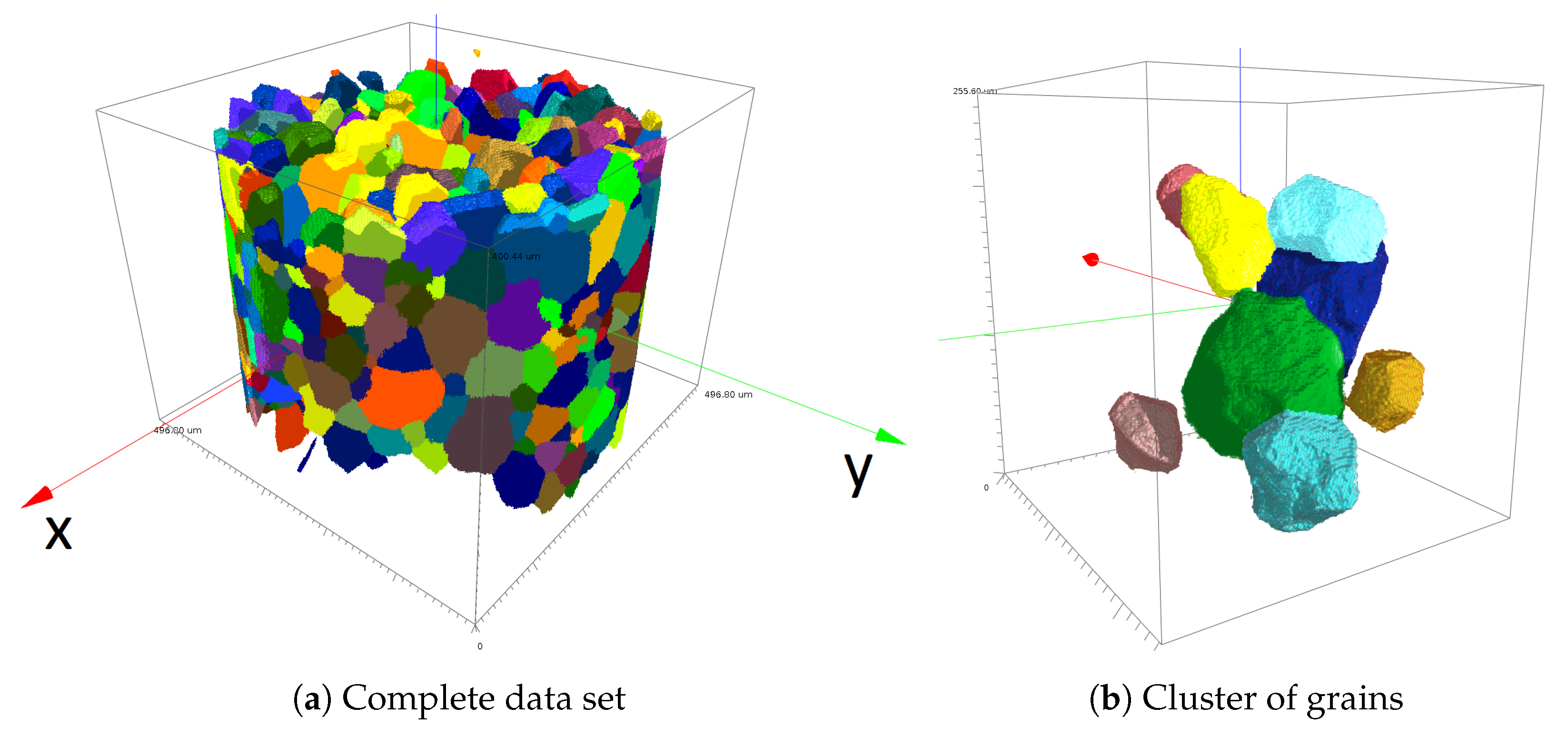
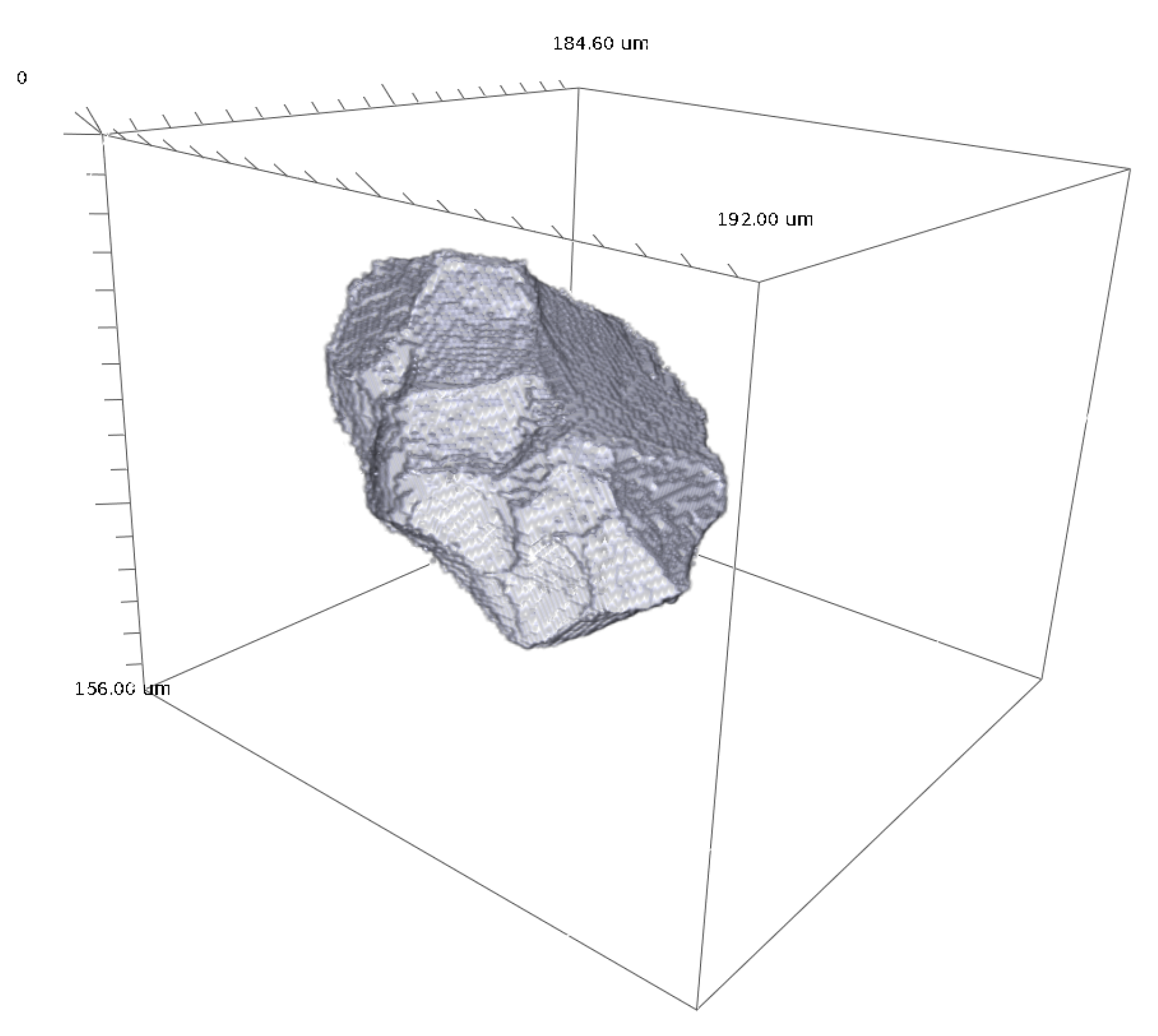
21]. These could be used for ultrasonic simulation, too. The DCT data also yields the crystallographic grain orientations. In order to exploit this structural information in the ultrasonic simulations, the spatial scattering functions need to be reformulated. In particular, the correlation function would have to account for eventually observed grain orientation correlations.
This paper is one step forward towards simulation of realistic grain noise in ultrasonic testing. Many more—most prominent considerable enlargement of the microstructure model realizations, incorporation of grain orientations, simulation of multiple scattering—wait to be conquered before simulated and experimental results can be compared quantitatively.

6. Conclusions

Ultrasonic testing is a popular, indispensable non-destructive testing technique. Its proper use relies heavily on simulations in order to interpret the received signals correctly. Simulation of ultrasonic wave propagation is therefore a vivid field of research.
This work focuses on polycrystalline materials and a method to account for the so-called grain noise caused by scattering of the propagating wave by the grain boundaries. Building on [13], we simulate backscattered wave contributions of the individual grains forming the polycrystal. To this end, the grain structure is modeled by a Laguerre tessellation model. Compared to the Voronoi tessellation used in previous attempts, using this more versatile type of model increases the effort for microstructure modelling considerably, enables however to capture the real grain size distribution much better. This is demonstrated here for two real metal alloy samples.
As discussed in Section 5 above, the method presented here needs generalizations in many ways before yielding simulated ultrasound signals that can be quantitatively compared to measured ones. We see it rather as a door opener towards realistic microstructure modeling in ultrasound simulation. We nevertheless achieved practically valuable results, too. In particular, the explicit relation of testing frequency, cell sizes, and Rayleigh boundary derived in Section 4.1.2 and Section 4.2.2. The spatial scattering functions and their shapes as shown in Figure 13 and Figure 18 shed a new light on the structure signal interaction and thus are of value on their own, too.
To summarize, we combined Hirsekorn’s [13] single scattering theory with explicit microstructure modeling using Laguerre tessellations to make considerable progress on the way to realistic grain noise simulation in ultrasonic testing.

Author Contributions

Conceptualization, D.D. and K.S.; methodology, D.D. and K.S.; software, D.D.; validation, D.D., K.S.; formal analysis, K.S.; investigation, D.D.; resources, D.D and K.S..; data curation, D.D.; writing–original draft preparation, D.D. and K.S.; writing–review and editing, D.D. and K.S.; visualization, D.D.; supervision, K.S.; project administration, D.D.; funding acquisition, D.D. All authors have read and agreed to the published version of the manuscript.

Funding

This project has been partially supported by the German Federal Ministry of Education and Research (BMBF) under grant 05M2013 (AniS) and 05M13RCA (AMSCHA). Also, Fraunhofer Society and DGZfP e.V. supported D.D. by scholarships.

Institutional Review Board Statement

Not applicable.

Informed Consent Statement

Not applicable.

Data Availability Statement

The data can be accessed on demand from the author.

Acknowledgments

The authors thank kindly Thomas Schwender at Fraunhofer Institute for Nondestructive Testing IZFP and Wolfgang Ludwig at European Synchrotron Radiation Facility ESRF for sharing the real microstructure data and making this investigation possible. We thank Claudia Redenbach and Joachim Ohser for helpful discussions and comments and Michael Godehardt for software solutions.

Conflicts of Interest

The authors declare no conflict of interest. The funders had no role in the design of the study; in the collection, analyses, or interpretation of data; in the writing of the manuscript, or in the decision to publish the results.

Abbreviations

The following abbreviations are used in this manuscript:
FFTFast Fourier Transformation
DCTDiffraction Contrast Tomography
ESRFEuropean Synchrotron Radiation Facility

References

  1. Gros, X. NDT Data Fusion; Knovel Library: London, UK, 1997. [Google Scholar]
  2. Spies, M.; Rieder, H.; Rauhut, M.; Kreier, P.; Innotest, A. Surface, Near-Surface and Volume Inspection of Cast Components Using Complementary NDT Approaches. In Proceedings of the 19th World Conference on Non-Destructive Testing 2016, Munich, Germany, 13–17 June 2016. [Google Scholar]
  3. Ashcroft, N.W.; Mermin, N.D. Festkörperphysik; De Gruyter: Berlin, Germany, 2001. [Google Scholar]
  4. Okazaki, K.; Conrad, H. Grain size distribution in recrystallized alpha-titanium. Trans. Jpn. Inst. Met. 1972, 13, 198–204. [Google Scholar] [CrossRef] [Green Version]
  5. Fan, Z.; Wu, Y.; Zhao, X.; Lu, Y. Simulation of polycrystalline structure with Voronoi diagram in Laguerre geometry based on random closed packing of spheres. Comput. Mater. Sci. 2004, 29, 301–308. [Google Scholar] [CrossRef]
  6. Mason, W.P.; McSkimin, H. Attenuation and scattering of high frequency sound waves in metals and glasses. J. Acoust. Soc. Am. 1947, 19, 464–473. [Google Scholar] [CrossRef]
  7. Truell, R.; Elbaum, C.; Chick, B.B. Ultrasonic Methods in Solid State Physics; Academic Press: New York, NY, USA, 1969. [Google Scholar]
  8. Stanke, F.E.; Kino, G. A unified theory for elastic wave propagation in polycrystalline materials. J. Acoust. Soc. Am. 1984, 75, 665–681. [Google Scholar] [CrossRef]
  9. Ishimaru, A. Wave Propagation and Scattering in Random Media; Academic Press: New York, NY, USA, 1978; Volume 1–2. [Google Scholar]
  10. Rose, J.H. Ultrasonic backscatter from microstructure. Rev. Prog. Quant. Nondestruct. Eval. Vol. 11B 1992, 11, 1677–1684. [Google Scholar]
  11. Dorval, V.; Jenson, F.; Corneloup, G.; Moysan, J. Accounting for structural noise and attenuation in the modeling of the ultrasonic testing of polycrystalline materials. In Proceedings of the AIP Conference Proceedings, Penang, Malaysia, 21–23 December 2010; Volume 1211, pp. 1309–1316. [Google Scholar]
  12. Ganjehi, L.; Dorval, V.; Jenson, F. Modelling of the ultrasonic propagation in polycrystalline materials. Acoustics 2012, 2012, 2621–2626. [Google Scholar]
  13. Hirsekorn, S. Theoretical description of ultrasonic propagation and scattering phenomena in polycrystalline structures aiming for simulations on nondestructive materials characterization and defect detection. In Proceedings of the 11th ECNDT Conference, Prague, Czech Republic, 6–11 October 2014. [Google Scholar]
  14. Bachmann, F.; Hielscher, R.; Schaeben, H. Grain detection from 2d and 3d EBSD data—Specification of the MTEX algorithm. Ultramicroscopy 2011, 111, 1720–1733. [Google Scholar] [CrossRef]
  15. Alpers, A.; Brieden, A.; Gritzmann, P.; Lyckegaard, A.; Poulsen, H.F. Generalized balanced power diagrams for 3D representations of polycrystals. Philos. Mag. 2015, 95, 1016–1028. [Google Scholar] [CrossRef] [Green Version]
  16. Šedivỳ, O.; Brereton, T.; Westhoff, D.; Polívka, L.; Beneš, V.; Schmidt, V.; Jäger, A. 3D reconstruction of grains in polycrystalline materials using a tessellation model with curved grain boundaries. Philos. Mag. 2016, 96, 1926–1949. [Google Scholar] [CrossRef]
  17. Šedivỳ, O.; Dake, J.M.; Krill III, C.E.; Schmidt, V.; Jäger, A. Description of the 3D morphology of grain boundaries in aluminum alloys using tessellation models generated by ellipsoids. Image Anal. Stereol. 2017, 36, 5–13. [Google Scholar] [CrossRef] [Green Version]
  18. Šedivỳ, O.; Westhoff, D.; Kopeček, J.; Krill III, C.E.; Schmidt, V. Data-driven selection of tessellation models describing polycrystalline microstructures. J. Stat. Phys. 2018, 172, 1223–1246. [Google Scholar] [CrossRef]
  19. Teferra, K.; Rowenhorst, D.J. Direct parameter estimation for generalised balanced power diagrams. Philos. Mag. Lett. 2018, 98, 79–87. [Google Scholar] [CrossRef]
  20. Petrich, L.; Staněk, J.; Wang, M.; Westhoff, D.; Heller, L.; Šittner, P.; Krill, C.E.; Beneš, V.; Schmidt, V. Reconstruction of Grains in Polycrystalline Materials From Incomplete Data Using Laguerre Tessellations. Microsc. Microanal. 2019, 25, 743–752. [Google Scholar] [CrossRef] [PubMed] [Green Version]
  21. Lyckegaard, A.; Lauridsen, E.M.; Ludwig, W.; Fonda, R.W.; Poulsen, H.F. On the Use of Laguerre Tessellations for Representations of 3D Grain Structures. Adv. Eng. Mater. 2011, 13, 165–170. [Google Scholar] [CrossRef]
  22. Ghoshal, G.; Turner, J.A. Numerical model of longitudinal wave scattering in polycrystals. IEEE Trans. Ultrason. Ferroelectr. Freq. Control 2009, 56, 1419–1428. [Google Scholar] [CrossRef] [PubMed]
  23. Shivaprasad, S.; Krishnamurthy, C.; Balasubramaniam, K. Modeling and simulation of ultrasonic beam skewing in polycrystalline materials. Int. J. Adv. Eng. Sci. Appl. Math. 2018, 10, 70–78. [Google Scholar] [CrossRef]
  24. Ryzy, M.; Grabec, T.; Sedlák, P.; Veres, I.A. Influence of grain morphology on ultrasonic wave attenuation in polycrystalline media with statistically equiaxed grains. J. Acoust. Soc. Am. 2018, 143, 219–229. [Google Scholar] [CrossRef] [Green Version]
  25. Van Pamel, A.; Brett, C.R.; Huthwaite, P.; Lowe, M.J. Finite element modelling of elastic wave scattering within a polycrystalline material in two and three dimensions. J. Acoust. Soc. Am. 2015, 138, 2326–2336. [Google Scholar] [CrossRef] [Green Version]
  26. Van Pamel, A.; Sha, G.; Rokhlin, S.I.; Lowe, M.J. Finite-element modelling of elastic wave propagation and scattering within heterogeneous media. Proc. R. Soc. A: Math. Phys. Eng. Sci. 2017, 473, 20160738. [Google Scholar] [CrossRef]
  27. Van Pamel, A.; Sha, G.; Lowe, M.J.; Rokhlin, S.I. Numerical and analytic modelling of elastodynamic scattering within polycrystalline materials. J. Acoust. Soc. Am. 2018, 143, 2394–2408. [Google Scholar] [CrossRef] [Green Version]
  28. Quey, R.; Dawson, P.; Barbe, F. Large-scale 3D random polycrystals for the finite element method: Generation, meshing and remeshing. Comput. Methods Appl. Mech. Eng. 2011, 200, 1729–1745. [Google Scholar] [CrossRef] [Green Version]
  29. Huthwaite, P. Accelerated finite element elastodynamic simulations using the GPU. J. Comput. Phys. 2014, 257, 687–707. [Google Scholar] [CrossRef] [Green Version]
  30. Standard ASTM E112; Standard Test Methods for Determining Average Grain Size. ASTM International: West Conshohocken, PA, USA, 2003.
  31. Margetan, F.J.; Nieters, E.; Haldipur, P.; Brasche, L.; Chiou, T.; Keller, M.; Degtyar, A.; Umbach, J.; Hassan, W.; Patton, T.; et al. Fundamental Studies of Nickel Billet Materials-Engine Titanium Consortium Phase II; National Technical Information Service (NTIS): Springfield, MA, USA, 2005.
  32. Walte, F.; Schwender, T.; Hirsekorn, S.; Schubert, F.; Spies, M. Reaktorsicherheitsforschung—Vorhaben-Nr.: 1501442 “Berechnung der Ultraschallstreuung für einen Verbesserten Nachweis von Rissartigen Fehlern in Austenitischen Schweissnähten. Phase 1: Berechnung der Ultraschallstreuung für 2DSchweissnahtmodelle”; Technical Report; Fraunhofer-Institut für Zerstörungsfreie Prüfverfahren IZFP: Saarbrücken, Germany, 2015. [Google Scholar]
  33. Tromans, D. Elastic anisotropy of HCP metal crystals and polycrystals. Int. J. Res. Rev. Appl. Sci 2011, 6, 462–483. [Google Scholar]
  34. Shannon, C.E. Communication in the presence of noise. Proc. IRE 1949, 37, 10–21. [Google Scholar] [CrossRef]
  35. Fließbach, T. Statistische Physik; Springer: Berlin/Heidelberg, Germany, 1993. [Google Scholar]
  36. Gaspard, P. Chaos, Scattering and Statistical Mechanics; Cambridge University Press: Cambridge, UK, 2005; Volume 9. [Google Scholar]
  37. Gubernatis, J.; Krumhansl, J. Macroscopic engineering properties of polycrystalline materials: Elastic properties. J. Appl. Phys. 1975, 46, 1875–1883. [Google Scholar] [CrossRef]
  38. Weaver, R.L. Diffusivity of ultrasound in polycrystals. J. Mech. Phys. Solids 1990, 38, 55–86. [Google Scholar] [CrossRef]
  39. Hirsekorn, S. Elastic properties of polycrystals: A review. Texture, Stress. Microstruct. 1990, 12, 1–14. [Google Scholar] [CrossRef] [Green Version]
  40. Hirsekorn, S. The scattering of ultrasonic waves by multiphase polycrystals. J. Acoust. Soc. Am. 1988, 83, 1231–1242. [Google Scholar] [CrossRef]
  41. Born, M. Quantenmechanik der stoßvorgänge. Z. Phys. 1926, 38, 803–827. [Google Scholar] [CrossRef]
  42. Torquato, S. Random Heterogeneous Materials: Microstructure and Macroscopic Properties; Springer Science & Business Media: Berlin/Heidelberg, Germany, 2013; Volume 16. [Google Scholar]
  43. Illian, J.; Penttinen, A.; Stoyan, H.; Stoyan, D. Statistical Analysis and Modelling of Spatial Point Patterns; John Wiley & Sons: Hoboken, NJ, USA, 2008; Volume 70. [Google Scholar]
  44. Man, C.S.; Paroni, R.; Xiang, Y.; Kenik, E.A. On the geometric autocorrelation function of polycrystalline materials. J. Comput. Appl. Math. 2006, 190, 200–210. [Google Scholar] [CrossRef]
  45. Arguelles, A.P.; Turner, J.A. Ultrasonic attenuation of polycrystalline materials with a distribution of grain sizes. J. Acoust. Soc. Am. 2017, 141, 4347–4353. [Google Scholar] [CrossRef] [PubMed]
  46. Dobrovolskij, D.; Hirsekorn, S.; Spies, M. Simulation of Ultrasonic Materials Evaluation Experiments Including Scattering Phenomena due to Polycrystalline Microstructure. Phys. Procedia 2015, 70, 644–647. [Google Scholar] [CrossRef]
  47. Chiu, S.N.; Stoyan, D.; Kendall, W.S.; Mecke, J. Stochastic Geometry and Its Applications; John Wiley & Sons: Hoboken, NJ, USA, 2013. [Google Scholar]
  48. Ohser, J.; Schladitz, K. 3D Images of Materials Structures: Processing and Analysis; John Wiley & Sons: Hoboken, NJ, USA, 2009. [Google Scholar]
  49. Xue, X.; Righetti, F.; Telley, H.; Liebling, T.M.; Mocellin, A. The laguerre model for grain growth in three dimensions. Philos. Mag. B 1997, 75, 567–585. [Google Scholar] [CrossRef]
  50. Kühn, M.; Steinhauser, M.O. Modeling and simulation of microstructures using power diagrams: Proof of the concept. Appl. Phys. Lett. 2008, 93, 034102. [Google Scholar] [CrossRef]
  51. Okabe, A.; Boots, B.; Sugihara, K.; Chiu, S.N. Spatial Tessellations: Concepts and Applications of Voronoi Diagrams; John Wiley & Sons: Hoboken, NJ, USA, 2009; Volume 501. [Google Scholar]
  52. Redenbach, C. Microstructure models for cellular materials. Comput. Mater. Sci. 2009, 44, 1397–1407. [Google Scholar] [CrossRef]
  53. Geißendörfer, M.; Liebscher, A.; Proppe, C.; Redenbach, C.; Schwarzer, D. Stochastic multiscale modeling of metal foams. Probabilistic Eng. Mech. 2014, 37, 132–137. [Google Scholar] [CrossRef]
  54. Kampf, J.; Schlachter, A.L.; Redenbach, C.; Liebscher, A. Segmentation, statistical analysis, and modelling of the wall system in ceramic foams. Mater. Charact. 2015, 99, 38–46. [Google Scholar] [CrossRef]
  55. Abdullahi, H.; Liang, Y.; Gao, S. Predicting the elastic properties of closed-cell aluminum foams: A mesoscopic geometric modeling approach. SN Appl. Sci. 2019, 1, 380. [Google Scholar] [CrossRef] [Green Version]
  56. Liebscher, A. Laguerre approximation of random foams. Philos. Mag. 2015, 95, 2777–2792. [Google Scholar] [CrossRef]
  57. Mościński, J.; Bargieł, M.; Rycerz, Z.; Jacobs, P. The force-biased algorithm for the irregular close packing of equal hard spheres. Mol. Simul. 1989, 3, 201–212. [Google Scholar] [CrossRef]
  58. Jodrey, W.S.; Tory, E.M. Simulation of random packing of spheres. Simulation 1979, 32, 1–12. [Google Scholar] [CrossRef]
  59. Bezrukov, A.; Stoyan, D.; Bargieł, M. Spatial statistics for simulated packings of spheres. Image Anal. Stereol. 2001, 20, 203–206. [Google Scholar] [CrossRef]
  60. Bezrukov, A.; Bargieł, M.; Stoyan, D. Statistical analysis of simulated random packings of spheres. Part. Part. Syst. Charact. Meas. Descr. Part. Prop. Behav. Powders Other Disperse Syst. 2002, 19, 111–118. [Google Scholar] [CrossRef]
  61. He, D.; Ekere, N. Computer Simulation of Powder Compaction of Spherical Particles. J. Mater. Sci. Lett. 1998, 17, 1723–1725. [Google Scholar] [CrossRef]
  62. Wu, Y.; Fan, Z.; Lu, Y. Bulk and interior packing densities of random close packing of hard spheres. J. Mater. Sci. 2003, 38, 2019–2025. [Google Scholar] [CrossRef]
  63. Rhines, F.; Patterson, B. Effect of the degree of prior cold work on the grain volume distribution and the rate of grain growth of recrystallized aluminum. Metall. Trans. A 1982, 13, 985–993. [Google Scholar] [CrossRef]
  64. Spies, M. Kirchhoff evaluation of scattered elastic wavefields in anisotropic media. J. Acoust. Soc. Am. 2000, 107, 2755–2759. [Google Scholar] [CrossRef]
  65. Červenỳ, V. Reflection/transmission laws for slowness vectors in viscoelastic anisotropic media. Stud. Geophys. Geod. 2007, 51, 391–410. [Google Scholar] [CrossRef]
  66. Auld, B. General electromechanical reciprocity relations applied to the calculation of elastic wave scattering coefficients. Wave Motion 1979, 1, 3–10. [Google Scholar] [CrossRef]
  67. Scheben, R.; Rieder, H.; Spies, M.; Götz, S. Kopplung von EFIT und GPSS zur Schnellen Ultraschallsimulation; NDT.net. German Society of NDT: Berlin, Germany, 2010; Volume 2. [Google Scholar]
  68. Spies, M. Prediction of Ultrasonic Flaw Signals and Model-to-Experiment Comparison. In Proceedings of the AIP Conference Proceedings, Salt Lake, UT, USA, 10–11 August 2005; Volume 760, pp. 1851–1858. [Google Scholar]
  69. Frigo, M.; Johnson, S.G. FFTW: An adaptive software architecture for the FFT. In Proceedings of the 1998 IEEE International Conference on Acoustics, Speech and Signal Processing, ICASSP’98 (Cat. No. 98CH36181). Seattle, WA, USA, 12–15 May 1998; Volume 3, pp. 1381–1384. [Google Scholar]
  70. Frigo, M.; Johnson, S.G. FFTW: Fastest Fourier Transform in the West; Astrophysics Source Code Library, 2012; Available online: https://ui.adsabs.harvard.edu/abs/2012ascl.soft01015F/abstract (accessed on 21 July 2021).
  71. Dagum, L.; Menon, R. OpenMP: An industry standard API for shared-memory programming. IEEE Comput. Sci. Eng. 1998, 5, 46–55. [Google Scholar] [CrossRef] [Green Version]
  72. Chandra, R.; Dagum, L.; Kohr, D.; Menon, R.; Maydan, D.; McDonald, J. Parallel Programming in OpenMP; Morgan Kaufmann: Burlington, MA, USA, 2001. [Google Scholar]
  73. Fraunhofer Institute for Industrial Mathematics ITWM. Cluster Homepage. 2021. Available online: https://www.itwm.fraunhofer.de/en/about-itwm/profile/central-it-infrastructure.html (accessed on 21 July 2021).
  74. Guo, Y.; Wang, B.; Hou, S. Aging precipitation behavior and mechanical properties of Inconel 617 superalloy. Acta Metall. Sin. (English Lett.) 2013, 26, 307–312. [Google Scholar] [CrossRef] [Green Version]
  75. Poulsen, H.F. An introduction to three-dimensional X-ray diffraction microscopy. J. Appl. Crystallogr. 2012, 45, 1084–1097. [Google Scholar] [CrossRef]
  76. Ludwig, W.; Reischig, P.; King, A.; Herbig, M.; Lauridsen, E.; Johnson, G.; Marrow, T.; Buffiere, J.Y. Three-dimensional grain mapping by x-ray diffraction contrast tomography and the use of Friedel pairs in diffraction data analysis. Rev. Sci. Instruments 2009, 80, 033905. [Google Scholar] [CrossRef] [PubMed] [Green Version]
  77. Ducousso-Ganjehi, L.; Châtillon, S.; Dorval, V.; Gilles-Pascaud, C.; Jenson, F. Modelling of the Ultrasonic Propagation in Titanium Alloy Materials. In Proceedings of the AeroNDT 2012 4th International Symposium on NDT in Aerospace, Augsburg, Germany, 13–14 November 2012; NDT.net. German Society of NDT: Berlin, Germany, 2012. [Google Scholar]
  78. Pilchak, A.L.; Li, J.; Rokhlin, S.I. Quantitative comparison of microtexture in near-alpha titanium measured by ultrasonic scattering and electron backscatter diffraction. Metall. Mater. Trans. A 2014, 45, 4679–4697. [Google Scholar] [CrossRef]
Figure 1. (a) Experimental setup assumed throughout including the particular choice of the global Cartesian coordinate system with top-down z-axis. The transducer is both transmitter and receiver for longitudinally polarized waves. In (b), dots mark the centers of the cells visualized in (a). The entire microstructure contributes to the received backscattered signal.
Acoustics 04 00010 g001
Figure 2. Proposed workflow.
Acoustics 04 00010 g002
Figure 3. Spatial scattering functions η ( ϑ , φ , 2 π 10   MHz ) for a single scatterer of size d eff = 54.5 µm in nickel. For every unit vector ( x 1 , x 2 , x 3 ) = sin ϑ cos φ , sin ϑ sin φ , cos ϑ , the function value η ( ϑ , φ , 2 π 10   MHz ) is represented here as the length of the vector in the corresponding direction.
Acoustics 04 00010 g003
Figure 4. 2D illustration for the construction of a Laguerre tessellation. The cyan circles are the generators with their weights, the red solid lines are the resulting faces of the Laguerre tessellation.
Acoustics 04 00010 g004
Figure 5. Volume renderings of force biased packings of 500 spheres in the unit window [ 0 , 1 ] 3 . Both with volume fraction V V = 52.1 % . Left: with constant sphere volume V = 0.011 . Right: with log-normally distributed sphere volumes ( μ v s = 7.67 and σ v s = 1.26 ).
Acoustics 04 00010 g005
Figure 6. Simulated frequency bandwidth with left bound f l = 0.5 f and right bound f r = 1.5 f .
Acoustics 04 00010 g006
Figure 7. Micrograph of the Inconel-617 under investigation, cell boundaries are emphasized by etching. Micrographs from [32] courtesy of Thomas Schwender (Fraunhofer IZFP).
Acoustics 04 00010 g007
Figure 8. Rendering of the DCT image data of the titanium sample. The imaged cylinder has a diameter of 518 µm and a height of 400 µm. In (a), boundary grains on top and bottom are removed to emphasize the shape and packing of grains. Subfigure (b) shows a cluster of grains from this data set. The grain colors are randomly chosen in order to visually separate neighboring grains and their shapes.
Acoustics 04 00010 g008
Figure 9. Visualization of the model fit for the Inconel-617. Left: Rendering of a realization of the random Laguerre tessellation with overall 2000 cells in a cube of edge length 3.91 mm, and volume 60 mm 3 . Right: 2D sections compared with the micrographs. The cells are visualized by false color mapping.
Acoustics 04 00010 g009
Figure 10. One of the original micrographs of the Inconel-617 and a rendering of a realization of the fitted Laguerre tessellation model with cv s = 3.5 and 2000 cells.
Acoustics 04 00010 g010
Figure 11. Histograms of maximal Feret diameters measured in the micrographs of the Inconel-617 and in 2D sections of realizations of the fitted Laguerre tessellation model with ( cv s = 3.5 and 2000 cells) slices.
Acoustics 04 00010 g011
Figure 12. Effective cell diameters in ten realizations of the Inconel-617 microstructure model. The solid and dashed horizontal lines correspond to the upper boundaries of the Rayleigh regime for the pressure and shear waves, respectively. Colors code the frequency, see legend. Clearly, the Rayleigh regime is violated in the 5 MHz case.
Acoustics 04 00010 g012
Figure 13. Spatial scattering function η P P ϑ , φ , 2 π f (in mm 3 ) for a single scatterer of size d eff = 329 µm, testing frequency (a) f = 0.5 MHz, d eff π f / v α = 0.15 and (b) f = 2.25 MHz, d eff π f / v α = 0.68 , respectively. Thus, according to Equation (16), for f = 2.25 , we are in the stochastic regime.
Acoustics 04 00010 g013
Figure 14. Backscattered signals (indicated by ten arbitrary colors) for a sequence of testing frequencies f = 0.5, 1, 2.25, and 5 MHz. The corresponding transducer is modeled by a circle with radius 3 mm, which emits and receives longitudinal waves.
Acoustics 04 00010 g014
Figure 15. Histograms of the grain volumes of the titanium sample and realizations of the model fitted to it ( cv s = 2.34 ).
Acoustics 04 00010 g015
Figure 16. Rendering of a non-convex grain observed in the DCT data of the titanium sample.
Acoustics 04 00010 g016
Figure 17. Effective cell diameters in ten realizations of the microstructure model for the titanium. Clearly, the Rayleigh regime is violated in the 50 MHz case.
Acoustics 04 00010 g017
Figure 18. Spatial scattering function η P P φ , ϑ , 2 π f (in mm 3 ) for a single scatterer size d eff = 36.4 µm, testing frequency (a) f = 5 MHz, d eff π f / v α = 0.09 and (b) f = 30 MHz, d eff π f / v α = 0.57 , respectively. Thus, according to Equation (16), for f = 30 we are in the stochastic regime.
Acoustics 04 00010 g018
Figure 19. Received backscattered signals in titanium for a sequence of testing frequencies f = 5, 10, 20, 30 and 50 MHz. The corresponding transducer is modeled as a circle with diameters 3 mm for frequency 50 MHz and 6 mm for all other frequencies, which emits and receives longitudinal waves.
Acoustics 04 00010 g019
Table 1. Elastic constants of the three considered alloys. Nickel [13] and Inconel-617 [32] feature face centered cubic (fcc) single crystal structures and titanium [33] a hexagonally closely packed (hcp) one. The material specific density ϱ represents the material in both conditions.
Single CrystalPolycrystalDensity
C 11 C 12 C 13 C 33 C 44 λ Lamé μ Lamé ϱ Featured
[ GPa ] [ GPa ] [ GPa ] [ GPa ] [ GPa ] [ GPa ] [ GPa ] [ g cm 3 ] in Section
nickel250--160118.5--8.905Section 2.1.2
Inconel-617243.3--163.05134.3134.582.98.36Section 3.2 and Section 4.1
titanium160661819046.576.1743.394.51Section 3.3 and Section 4.2
Table 2. Ensemble averaged elastic constants (in GPa 2 ) as used for the calculation of backscattering coefficients [40].
AbbreviationEnsemble Averaged Elastic ConstantsNickelInconel-617Titanium
A 1 ( C 1133 ) 2 370.44 608.15 39.86
A 2 ( C 3333 ) 2 658.55 1 081.12 30.96
A 4 ( C 1233 ) 2 205.80 337.86 29.56
A 5 C 1133 C 3333 329.27 540.58 17.84
A 6 ( C 1333 ) 2 411.59 675.72 7.14
A 7 C 1113 C 2213 102.90 168.93 12.71
A 8 ( C 1213 ) 2 205.80 337.86 15.53
A 9 C 1113 C 1333 308.69 506.79 3.79
A 10 ( C 1313 ) 2 370.44 608.15 21.16
Table 3. Summary of the Inconel-617 microstructure model ( cv s = 3.5 and 16,000 cells) realizations.
Realization std i ( V eff ( C i ) ) min i ( d eff ( C i ) ) max i ( d eff ( C i ) )
Nr. ( mm 3 ) ( μ m ) ( μ m )
10.0715621039
20.0739641131
30.069345 967
40.0693571002
50.0723601032
60.070162 896
70.068459 956
80.0729591137
90.066961 860
100.0656561099
mean0.070058.51011
Table 4. Results for the titanium model realizations ( cv s = 2.34 and 17,344 cells).
Nr. std i ( C i ) min i ( d eff ( C i ) ) max i ( d eff ( C i ) )
in 10 4 ( μ m 3 ) ( μ m ) ( μ m )
15.5405 79
25.6077 81
35.8887 83
46.4267108
55.9087 88
65.6156 81
76.5097112
86.4967104
95.9227 91
105.8977 81
mean5.9806.790.8
Publisher’s Note: MDPI stays neutral with regard to jurisdictional claims in published maps and institutional affiliations.

