Article

Finite Element Analyses of the Modified Strain Gradient Theory Based Kirchhoff Microplates

Mechanical Engineering Department, Middle East Technical University, Dumlupınar Bulvarı 1, 06800 Ankara, Turkey
*
Author to whom correspondence should be addressed.
Surfaces 2021, 4(2), 115-156; https://doi.org/10.3390/surfaces4020014
Submission received: 27 March 2021 / Revised: 24 April 2021 / Accepted: 26 April 2021 / Published: 14 May 2021
(This article belongs to the Special Issue Interfaces in Materials Science and Engineering)

Abstract

:
In this contribution, the variational problem for the Kirchhoff plate based on the modified strain gradient theory (MSGT) is derived, and the Euler-Lagrange equations governing the equation of motion are obtained. The Galerkin-type weak form, upon which the finite element method is constructed, is derived from the variational problem. The shape functions which satisfy the governing homogeneous partial differential equation are derived as extensions of Adini-Clough-Melosh (ACM) and Bogner-Fox-Schmit (BFS) plate element formulations by introducing additional curvature degrees of freedom (DOF) on each node. Based on the proposed set of shape functions, 20-, 24-, 28- and 32- DOF modified strain gradient theory-based higher-order Kirchhoff microplate element are proposed. The performance of the elements are demonstrated in terms of various tests and representative boundary value problems. Length scale parameters for gold are also proposed based on experiments reported in literature.

1. Introduction

Micro- and nano-electro-mechanical systems (MEMS/NEMS) are essential components of advanced technologies [1,2,3,4,5,6]. They are used as pressure and acceleration sensors in many products such as airbag actuators, gyros, switches and mechanical filters as RF-MEMS, image processing tools as optical-MEMS, intrauterine sensors and biochemical detectors as bio-MEMS and so on [5,7,8,9,10].
The mechanical behavior of MEMS and NEMS devices diverge from that of macro-devices as their sizes get smaller. This phenomenon is known as size effect or scale effect, resulting in stiffening in mechanical response as the structural length-scale tends to the material length-scale describing the microstructure. The theoretical modelling of size effects in terms of nonlocal continuum models dates back to the early works of [11,12,13,14,15,16,17,18,19,20,21,22]. The concepts of couple stresses, micropolar elasticity, micromorphic theory, nonlocal elasticity originate from these pioneering works. Within this context, the term micromorphic theory is coined for the first time by Eringen and Suhubi [23,24]. A more specific form, the Strain Gradient Theories (SGT) originate from the works of Mindlin et al. [13,14,15,20], Toupin [22] and Koiter [19]. These are in general called the higher-order theories in which the internal potential of a solid body depends only on strains but also higher-order strains as strain gradients. Fleck and Hutchinson [25,26,27] extended SGT, pioneering the framework of modern higher-order theories. The Modified Strain Gradient Theory (MSGT) of Lam et al. [28] decreased the number of length-scale parameters from five to three in SGT using new equilibrium conditions. Another variation with one length-scale parameter is also used as the Modified Couple Stress Theory (MCST) of Yang et al. [29]. Although many studies exist regarding application and implementation of higher-order theories to microbeams, microplates did not receive much attention so far [30,31,32]. Reddy [33] proposed a nonlocal plate formulation extending the nonlocal continuum theory of Eringen [34]. Phadikar and Pradhan developed finite element formulations of Euler-Bernoulli beams and Kirchhoff plates for nonlocal elasticiy using one nonlocal parameter [35]. Wang et al. [36] developed a model for SGT for Kirchhoff microplates and solved various bending problems for specific boundary conditions [37]. SGT has also been implemented in Kirchhoff plates via isogeometric analyses successfully [38,39,40]. Arefi and Zenkour analyzed magneto–electro–thermo-mechanical bending and free vibration behavior of a sandwich microbeam [41,42] and microplate using SGT [43]. They also analyzed a three-layered microbeam using SGT and three-unknown shear and normal deformation theory [44]. Sohby and Zenkour [45] analyzed hygrothermal behavior of exponentially graded microplates on elastic foundations with MCST, whereas nonlocal SGT is also utilized [46]. Movassagh and Mahmoodi [47] derived the formulation for application of Kirchhoff plate theory to MSGT and further developed a Kirchhoff plate model in MSGT using extended Kantarovich method. Sahmani and Ansari analyzed FGM’s based on shear deformation plate theory and MSGT [48]. Li et al. studied the bending behavior of bi-layered Kirchhoff microplates based on SGT [49].
The above-mentioned contributions provided great insight towards the essense of size-dependent theories, and are oriented towards analytical modelling applicable for either ideal geometries or ideal boundary conditions that would be applicable to extremely limited conditions. However, stable and convergent finite element implementations allow the analysis and design of MEMS switches of various geometries and boundary conditions. Recently, there is considerable effort regarding the development of finite element formulations for size-dependent theories using Kirchhoff plates. Babu and Patel [50,51] developed a quadrilateral Kirchhoff plate element for second-order strain gradient theory proposed by Ru and Aifantis [52,53]. Beheshti [54] used the same formulation to develop four types of rectangular elements with different nodal degree of freedoms. Bacciocchi et al. used nonlocal strain gradient theory to formulate a finite element method and used it for laminated nanoplates in bending [55] and in hygro-thermal environment [56].
The main objective of this contribution is to propose novel finite element formulations for Kirchhoff microplates in a specific branch of strain gradient theories, i.e., MSGT proposed by Lam et al. [28], which contains three length scale parameters for modelling size effects. The key features and contributions of this study are;
(i)
to introduce a variational formulation for microplates based on the Kirchhoff kinematics and the modified strain gradient theory,
(ii)
to formulate 20- and 24-degree of freedom (DOF) rectangular micro-plate element formulations from serendipity-type higher-order basis functions enriched by sinh ( x , y ) and cosh ( x , y ) terms as extensions of the Adini-Clough-Melosh [57,58] element and Bogner-Fox-Schmit [59] element respectively,
(iii)
to further formulate 28- and 32-degree of freedom (DOF) rectangular micro-plate element formulations from 20- and 24-degree of freedom (DOF) rectangular micro-plate element formulations respectively,
(iv)
to assess the convergence of the derived element formulations and elaborate on the continuity requirements,
(v)
investigate the performance of the element through realistic MEMS switch geometries, and
(vi)
to contribute to the analysis of MEMS devices with various boundary conditions, particularly in the domain of RF-MEMS made of gold by proposing length scale parameters based on the proposed formulations.
Particularly, we propose a set of shape functions that satisfies the exact solution to the homogeneous PDE governing the MSGT based higher-order Kirchhoff plate theory. To this end, higher-order Kirchhoff plate finite elements for bending are developed based on Modified Strain Gradient Theory (MSGT). Then the weak form, from which the finite element formulations are constructed, is derived from variational principle or the principle of minimum potential energy. Using these elements, length scale parameters of gold are identified based on experiments reported in literature [60]. As a result, considerable size effect for gold microplate structures is revealed.
The proposed set of shape functions for the 20-DOF element naturally depends on a twenty-term basis function consisting of twelve monomials applicable to conventional rectangular Kirchhoff finite elements, and eight additional terms based on hyperbolic sine and hyperbolic cosine terms for the higher-order portion of the problem. The said twelve monomials belong to the simplest classical rectangular element which has twelve degrees of freedom, as known as Adini-Clough-Melosh (ACM) element [57,58]. This element does not pass the patch test but is convergent when used as rectangular finite elements [61]. For 24-DOF element, sixteen monomials applicable to a different classical element are used. This element has sixteen degrees of freedom and is known as Bogner-Fox-Schmit (BFS) element [59]. The additional eight terms are the same hyperbolic terms discussed above for 20-DOF element. The remaning 28- and 32-DOF elements are extensions of the 20- and 24-DOF elements - each with additional eight DOFs.
In order to assess the performance of the proposed higher-order finite element formulations, realistic NEMS switch geometries from literature are analyzed and the results are compared to those obtained from classical Kirchhoff plate theory. Yet, the dependence of the results on the aspect ratio is also investigated for the quadrilateral element formulation for the classical and higher-order Kirchhoff plates. It must be emphasized that the higher-order finite elements developed within this study are applicable to rectangular elements, as they fail to pass the patch test. However, this does not reduce the implementation of these elements in the community, given most of the MEMS and NEMS devices can be modelled by rectangular elements [6,62,63,64]. As a novel aspect, it is shown that 20-DOF rectangular elements can be used to model these types of MEMS structures. Chamfers at the edges and corners can also be found in some MEMS and NEMS devices [2,65,66,67]. Circular shapes are even possible in several applications such as micropumps and pressure sensors [68,69,70]. Again, as a novel aspect, it is shown that 24-DOF rectangular elements can be used in rectangular-triangular meshes, complementing with the readily available Bell elements [71]. With this method, any planar finite element domain of any shape can be modelled with the said rectangular and triangular elements [72].
This manuscript is organized as follows: In Section 2, the variational principle governing the higher-order Kirchhoff plate theory-based on the modified strain gradient theory is described and the respective Euler-Lagrange equations are derived. Section 3 is devoted to the novel finite element formulation of microplates based on the modified strain gradient theory of nonlocal elasticity. In Section 4, the performance of the proposed element is assessed through representative benchmark numerical examples. The paper ends with concluding remarks in Section 5.

2. Theory: Local and Nonlocal Kirchhoff Plate Theory

2.1. Variational Formulation of Nonlocal Elasticity

2.1.1. The Strain Gradient Theory

The free energy function for the linear isotropic solid is
ψ ( ε ) = 1 2 λ ( tr ε ) 2 + μ ε : ε where ε = 1 2 ( u + T u )
where is the strain tensor. Herein, λ and μ are the first Lamé constant and the shear modulus respectively [32].
The nonlocal elasticity is implemented by the addition of higher-order strains into the free energy function in the sense of Mindlin [15]
ψ = ψ ˜ ( ε , η ) where η = u
where is the second gradient of the displacement field where u is the displacement field. For isotropic materials, the free energy function can be written in an additive format
ψ ˜ ( ε , η ) = ψ loc ( ε ) + ψ nlo ( η ) , where ψ loc ( ε ) = 1 2 λ t r ε 2 + μ ε : ε
and
ψ nlo ( η ) = a 1 η : 1 · η : 1 + a 2 1 : η · η : 1 + a 3 1 : η · 1 : η + a 4 η : η + a 5 ( η     η T 13 )
where are the local and nonlocal parts of the free energy function, respectively, see references [20,26]. In the most general case, five additional material parameters a i exist. From (3) 1 , the first variation of the free energy can be derived as
δ ψ = σ : δ ε + τ     δ η where σ : = ε ψ loc ( ε ) and τ : = η ψ nlo ( η )
where are the second order and third order stress tensors as work conjugates of the second order strain tensor ε and the third order strain tensor η , respectively.

2.1.2. The Modified Strain Gradient Theory

Lam et al. [28] proposed a more specific form of the ansatz (2) and (5)
ψ = ψ ˜ ( ε , ϵ , η 1 , χ ) leading to δ ψ = σ : δ ε + p · δ ε + τ     δ η 1 + m : δ χ ,
where σ , p , τ , m are the local stress tensor, pressure gradient vector, the double stress tensor, and the couple stress tensor,
σ : = ε ψ loc ( ε ) , p : = ϵ ψ nlo ( η , ϵ , χ ) , τ : = η 1 ψ nlo ( η , ϵ , χ ) , and m : = χ ψ nlo ( η , ϵ , χ )
as the work conjugates of the strain tensor ε , dilatation gradient ϵ = tr ε , deviatoric stretch gradient tensor η 1 , and curvature tensor χ such that
η 1 = 1 3 p ε 1 15 1 ϵ 1 15 2 1 tr ( ε ) + 1 ϵ T 13 + 2 1 tr ( ε ) T 13 + 1 ϵ T 23 + 2 1 tr ( ε ) T 23 , and χ : = 1 2 ϑ + T ϑ ] with ϑ : = 1 2 curl u .
Therein, p is the permutational gradient defined as p ε = ε j k , i + ε k i , j + ε i j , k . The higher-order strain metrics are the deviatoric stretch gradient tensor η 1 in addition to the rotation gradient tensor or the curvature tensor χ . ϵ is the dilatation gradient vector. The total internal energy for the modified strain gradient theory of Lam et al. [28] then takes the following form
Π i n t ( u ) : = B ψ ˜ ( ε , ϵ , χ ) V . ψ nlo = ψ ˜ ( ϵ , χ ) = μ l 0 2 ϵ · ϵ + μ l 1 2 η 1     η 1 + μ l 1 2 χ : χ .
The Euler-Lagrange equations of the minimization principle then reads
div σ + [ div p ] + div [ div τ ] + 1 2 curl [ div m ] + ρ 0 b = 0 .
Herein, the corresponding stress measures as work conjugates of the strain measures ε , ϵ and χ respectively are
σ = λ t r ε 1 + 2 μ ε , p = 2 μ l 0 2 ϵ , τ = 2 μ l 1 2 η 1 and m = 2 μ l 2 2 χ ,
where l 0 , l 1 , l 2 are the three length scale parameters of the modified strain gradient theory associated with the higher-order strains ϵ , η 1 , and χ , respectively.

2.2. Classical Kirchhoff Plate Theory

Kirchhoff plate theory is the extension of Euler-Bernoulli beam theory to two-dimensional space. Accordingly, rotations are assumed to be small and plane sections are assumed to remain plane and perpendicular to the neutral axis. Consequently, the displacement field simplifies to
u x ( x , y , z ) = z w x , u y ( x , y , z ) = z w y , u z ( x , y ) = w ,
where the plate axes and geometry are as defined as in Figure 1a and w = w ( x , y ) . Therein, L is the length, W is the width, and h is the thickness of the plate. The out-of-plane rotations and the curvatures can be described as
θ x = w y , θ y = w x , κ x x = 2 w x 2 , κ y y = 2 w y 2 , and κ x y = κ y x = 2 2 w x y .
The small-strain linear isotropic material response leads to the constitutive relation between the moment and the curvature
M : = E κ where M x x M y y M x y = D 1 ν 0 ν 1 0 0 0 1 2 ( 1 + ν ) κ x x κ y y κ x y , and D = E h 3 / 12 ( 1 ν 2 ) .
Herein, D, E, ν are the isotropic plate rigidity, modulus of elasticity and Poisson’s ratio, respectively. The displacement vector u consists of vertical displacements w and rotations θ and surface traction vector t consists of shear forces V and moments M as given in Figure 1b. Due to kinematic equations, shearing, twisting and membrane effects are neglected in the strain energy equation. Therefore strain energy is governed by bending action solely.
For a Kirchhoff plate, the internal and the external potentials read
Π i n t = 1 2 B M κ d A and Π e x t = B q ¯ w ¯ d A + B t V ¯ w ¯ d s + B t M ¯ · θ ¯ d s ,
where
M ¯ = M ¯ x x M ¯ y y and θ ¯ = θ ¯ x θ ¯ y .
The first variation of the total potential Π has to vanish at the equilibrium state. Hence
δ Π = B δ κ x x D ( κ x x + ν κ y y ) + δ κ y y D ( κ y y + ν κ x x ) + δ κ x y D 1 2 ( 1 ν ) κ x y d A B q ¯ δ w ¯ d A + B t V ¯ δ w ¯ d s + B t M ¯ δ θ ¯ d s = 0 .
The Euler-Lagrange equation of the minimization principle can then be derived as
D 4 w ( x , y ) x 4 + 2 2 w ( x , y ) x 2 y 2 + 4 w ( x , y ) y 4 q ( x , y ) = 0 or D 2 2 ( w ) q = 0 ,
where 2 2 ( ) is the biharmonic operator. The Dirichlet (essential) and Neumann (natural) boundary conditions are respectively,
1 . w = w ¯ θ x = θ ¯ x θ y = θ ¯ y at B u , 2 . V = V ¯ M x x = M x x ¯ M y y = M y y ¯ at B t .

2.3. Modified Strain Gradient Theory for Kirchhoff Plates

With the displacement field given in Equation (12) and kinematic relations given in Equation (13) valid, an additional set of higher-order out-of-plane curvatures are defined as
ϱ x x x = 3 w x 3 , ϱ x x y = 3 w x 2 y , ϱ x y y = 3 w x y 2 , and ϱ y y y = 3 w x 3 .
The constitutive relations between the moment & curvature and higher-order forces & higher-order curvatures are, respectively
M : = E C κ : M x x M y y M x y = d 1 d 2 0 d 2 d 1 0 0 0 d 3 κ x x κ y y κ x y and Q : = E H ϱ : Q x x x Q x x y Q x y y Q y y y = d 4 0 d 5 0 0 d 6 0 d 5 d 5 0 d 6 0 0 d 5 0 d 4 ϱ x x x ϱ x x y ϱ x y y ϱ y y y
where
d 1 = D + μ h 2 l 0 2 + 8 15 l 1 2 + l 2 2 , d 2 = D ν + μ h 2 l 0 2 2 15 l 1 2 l 2 2 , d 3 = 2 D ( 1 ν ) + μ h 4 3 l 1 2 + 4 l 2 2 , d 4 = μ h 3 l 0 2 6 + l 1 2 15 , d 5 = μ h 3 l 0 2 6 l 1 2 10 , d 6 = μ h 3 l 0 2 6 + l 1 2 5 .
Derivation of the above equations are given in Appendix A. For the MSGT based higher-order Kirchhoff plate, the internal potential reads
Π i n t = 1 2 B M · κ + Q · ϱ d A .
The external potential reads
Π e x t = B q ¯ w ¯ d A + B t V ¯ w ¯ d s + B t M ¯ θ ¯ d s + B t Q ¯ κ ¯ d s where Q ¯ = Q ¯ x x x Q ¯ y y y and κ ¯ = κ ¯ x x κ ¯ y y .
Q is therefore the work conjugate of the curvature κ , similar to the work conjugate couples Vw and M θ . The first variation of the internal potential leads to
δ Π i n t = B δ κ x x ( d 1 κ x x + d 2 κ y y ) + δ κ y y ( d 2 κ x x + d 1 κ y y ) + δ κ x y d 3 κ x y + δ ϱ x x x ( d 4 ϱ x x x d 5 ϱ x y y ) + δ ϱ x x y ( d 6 ϱ x x y + d 5 ϱ y y y ) + δ ϱ x y y ( d 5 ϱ x x x + d 6 ϱ x y y ) + δ ϱ y y y ( d 5 ϱ x x y + d 4 ϱ y y y ) d A .
Similarly, the first variation of the external work potential can be derived as
δ Π e x t = B q ¯ δ w ¯ d A + B t V ¯ δ w ¯ d s + B t M ¯ δ θ ¯ d s + B t Q ¯ δ κ ¯ d s .
The principle of minimum potential energy also requires the variation of the total potential to vanish at equilibrium. The Euler-Lagrange equation of the minimization principle can be derived as follows
d 1 4 w x 4 + 2 4 w x 2 y 2 + 4 w y 4 d 4 6 w x 6 + 3 6 w x 4 y 2 + 3 6 w x 2 y 4 + 6 w y 6 q = 0 .
The Dirichlet and Neumann boundary conditions are respectively,
1 . w = w ¯ θ x = θ ¯ x θ y = θ ¯ y κ x = κ ¯ x κ y = κ ¯ y at B u , 2 . V = V ¯ M x x = M x x ¯ M y y = M y y ¯ Q x = Q x ¯ Q y = Q y ¯ at B t .

3. The Microplate Finite Element Formulation

The finite element formulation for the classical plate theory and the modified strain gradient theory will be obtained using the variational formulations presented in Section 2. The proposed finite element formulation is derived by first proposing additional higher-order DOF’s. Then, homogeneous solutions that satisfy Equation (18) are proposed and the shape functions are checked. From the relevant shape functions, local element stiffmess matrices are derived.

3.1. 12-Dof Adini-Clough-Melosh Element for Classical Kirchhoff Plates

Let us consider a classical Kirchhoff plate element domain B e as depicted in Figure 1a. The generalized displacements at the element nodes are prescribed as
1 . w = w 1 , θ x = θ x 1 and θ y = θ y 1 at x = 0 and y = 0 , 2 . w = w 2 , θ x = θ x 2 and θ y = θ y 2 at x = L and y = 0 , 3 . w = w 3 , θ x = θ x 3 and θ y = θ y 3 at x = L and y = W , 4 . w = w 4 , θ x = θ x 4 and θ y = θ y 4 at x = 0 and y = W ,
see also Figure 2a. Similarly, the generalized nodal force resultants are prescribed as
1 . V = V 1 , M x = M x 1 and M y = M y 1 at x = 0 and y = 0 , 2 . V = V 2 , M x = M x 2 and M y = M y 2 at x = L and y = 0 , 3 . V = V 3 , M x = M x 3 and M y = M y 3 at x = L and y = W , 4 . V = V 4 , M x = M x 4 and M y = M y 4 at x = 0 and y = W ,
see also Figure 2b. Accordingly, the vector field containing the nodal displacement vector d and the nodal force vector f read
d T = w 1 θ x 1 θ y 1 . . . w 4 θ x 4 θ y 4 , f T = V 1 M x 1 M y 1 . . . V 4 M x 4 M y 4 .
The displacement field w ( x , y ) within the element domain B e is interpolated as
w ( x , y ) = N d = i = 1 n DOF j = 1 n nodes N i j d i j where N = N 1 1 N 2 1 N 3 1 . . . N 1 4 N 2 4 N 3 4 ,
where is the row vector including the set of interpolation/shape functions. n DOF = 3 is the number of degrees of freedom (DOFs) per node and n nodes = 4 is the number of nodes per element, with N i j , i denoting the relevant DOF of the node and j denoting the relevant node. The number of DOFs per element is hence 12. The homogenous solution of the partial differential Equation (18) is
w ( x , y ) = a 1 + a 2 x + a 3 y + a 4 x 2 + a 5 x y + a 6 y 2 + a 7 x 3 + a 8 x 2 y + a 9 x y 2 + a 10 y 3 + a 11 x 3 y + a 12 x y 3 .
The 12 DOF plate element with such shape functions is known as the ACM quadrilateral [73]. The first three of the twelve shape functions are given in Figure 3, where the remaining nine are symmetric with respect to two principal centroidal axes x ¯ and y ¯ around the geometric center of the element. The analytic expressions for the ACM shape functions are given in Appendix B, see also [73]. The ACM element does not satisfy the C 1 continuity requirement, and therefore it is a non-conforming element [61].
The displacement w ( x , y ) , rotation { θ x , θ y } , and the curvature { κ x , κ y , κ x y } fields (13) can be approximated as
w ( x , y ) = N ( x , y ) d , θ x ( x , y ) = N ( x , y ) y d , θ y ( x , y ) = N ( x , y ) x d , κ x x ( x , y ) = 2 N ( x , y ) y 2 d , κ y y ( x , y ) = 2 N ( x , y ) x 2 d , κ x y ( x , y ) = 2 N ( x , y ) x y d .
Consequently, the variation of the field variables (34) are
δ w ( x , y ) = N ( x , y ) δ d , δ θ x ( x , y ) = N ( x , y ) y δ d , δ θ y ( x , y ) = N ( x , y ) x δ d , δ κ x x ( x , y ) = 2 N ( x , y ) y 2 δ d , δ κ y y ( x , y ) = 2 N ( x , y ) x 2 δ d , δ κ x y ( x , y ) = 2 N ( x , y ) x y δ d .
Incorporation of the discrete counterpart of the curvature in Equation (34) and their variations (35) into (17), we obtain
δ Π = A e = 1 n δ d e T k e d e A e = 1 n δ d e T f e = 0 ,
where
k e = B C N T E C N d A and f e = B N T q ( x , y ) d A
where are the element stiffnes matrix and the element nodal force vectors. For the sake of convenience the loading terms on the boundary are omitted for f e . Therein, the operator C is defined as
C = 2 x 2 2 2 x y 2 y 2 T ,
and A refers to the standard assembly of element contributions at the local element nodes where n denotes the total number of elements. In Equation (47) the strain-displacement matrix is C N as given in Appendix D.
The global stiffness matrix, generalized nodal displacement vector and the generalized force vector assembled from local force vectors read
K = A e = 1 n k e , D = A e = 1 n d e and F = A e = 1 n f e ,
respectively. No variation exists δ d = 0 at essential boundary B u where the displacements are prescribed d = d ¯ . The equilibrium is satisfied for arbitrary variation of the displacement δ d leading to the set of linear algebraic equations
K D = F .

3.2. 16-Dof Bogner-Fox-Schmit Element for Classical Kirchhoff Plates

For a classical Kirchhoff plate element the generalized displacements at the element nodes are prescribed as
1 . w = w 1 , θ x = θ x 1 , θ y = θ y 1 , and κ x y = κ x y 1 , at node 1 , 2 . w = w 2 , θ x = θ x 2 , θ y = θ y 2 , and κ x y = κ x y 2 , at node 2 , 3 . w = w 3 , θ x = θ x 3 , θ y = θ y 3 , and κ x y = κ x y 3 , at node 3 , 4 . w = w 4 , θ x = θ x 4 , θ y = θ y 4 , and κ x y = κ x y 4 , at node 4 ,
see also Figure 4a. Similarly, the generalized nodal force resultants are prescribed as
1 . V = V 1 , M x = M x 1 , M y = M y 1 , and M x y = M x y 1 , at node 1 , 2 . V = V 2 , M x = M x 2 , M y = M y 2 , and M x y = M x y 2 , at node 2 , 3 . V = V 3 , M x = M x 3 , M y = M y 3 , and M x y = M x y 3 , at node 3 , 4 . V = V 4 , M x = M x 4 , M y = M y 4 , and M x y = M x y 4 , at node 4 ,
see also Figure 4b.
The nodal displacement vector d and the nodal force vector f are
d T = w 1 θ x 1 θ y 1 κ x y 1 . . . w 4 θ x 4 θ y 4 κ x y 4 , f T = V 1 M x 1 M y 1 M x y 1 . . . V 4 M x 4 M y 4 M x y 4 .
The displacement field w ( x , y ) within the element domain is interpolated as
w ( x , y ) = N d = i = 1 n DOF j = 1 n nodes N i j d i j where N = N 1 1 N 2 1 N 3 1 N 4 1 . . . N 1 4 N 2 4 N 3 4 N 4 4 ,
where N is the row vector including the set of interpolation/shape functions, n DOF = 4 is the number of degrees of freedom (DOFs) per node and n nodes = 4 is the number of nodes per element. For N i j , i denotes the relevant DOF of the node and j denotes the relevant node. The number of DOFs per element is hence 16. The homogenous solution of the partial differential biharmonic plate equation is
w ( x , y ) = a 1 + a 2 x + a 3 y + a 4 x 2 + a 5 x y + a 6 y 2 + a 7 x 3 + a 8 x 2 y + a 9 x y 2 + a 10 y 3 + a 11 x 3 y + a 12 x 2 y 2 + a 13 x y 3 + a 14 x 2 y 3 + a 15 x 3 y 2 + a 16 x 3 y 3 .
Incorporation of these into the total functional, we obtain
δ Π = A e = 1 n δ d e T k e d e A e = 1 n δ d e T f e = 0 ,
where
k e = B C N T E C N d A and f e = B N T q ( x , y ) d A
are the element stiffness matrix and the element nodal force vectors.
The global stiffness matrix, generalized nodal displacement vector and the generalized force vector are assembled from local force vectors in a similar manner as described in Section 3.1.

3.3. New 20-Dof Finite Element Formulation for Msgt-Based Kirchhoff Microplates

Let us now consider a MSGT-based Kirchhoff plate element domain B e . The generalized displacements at the element nodes are prescribed as
1 . w = w 1 , θ x = θ x 1 , θ y = θ y 1 , κ x = κ x 1 and κ y = κ y 1 , at x = 0 and y = 0 , 2 . w = w 2 , θ x = θ x 2 , θ y = θ y 2 , κ x = κ x 2 and κ y = κ y 2 , at x = L and y = 0 , 3 . w = w 3 , θ x = θ x 3 , θ y = θ y 3 , κ x = κ x 3 and κ y = κ y 3 , at x = L and y = W , 4 . w = w 4 , θ x = θ x 4 , θ y = θ y 4 , κ x = κ x 4 and κ y = κ y 4 , at x = 0 and y = W ,
see also Figure 5a. Similarly, the generalized nodal force resultants are prescribed as
1 . V = V 1 , M x = M x 1 , M y = M y 1 , Q x = Q x 1 and Q y = Q y 1 , at x = 0 and y = 0 , 2 . V = V 2 , M x = M x 2 , M y = M y 2 , Q x = Q x 2 and Q y = Q y 2 , at x = L and y = 0 , 3 . V = V 3 , M x = M x 3 , M y = M y 3 , Q x = Q x 3 and Q y = Q y 3 , at x = L and y = W , 4 . V = V 4 , M x = M x 4 , M y = M y 4 , Q x = Q x 4 and Q y = Q y 4 , at x = 0 and y = W ,
see Figure 5b for relevant nomenclature. The element nodal displacement vector d and the element nodal force vector f of the higher-order Kirchhoff plate are, respectively,
d T = w 1 θ x 1 θ y 1 κ x 1 κ y 1 . . . w 4 θ x 4 θ y 4 κ x 4 κ y 4 , f T = V 1 M x 1 M y 1 Q x 1 Q y 1 . . . V 4 M x 4 M y 4 Q x 4 Q y 4 ,
where the nodal bi-axial curvatures and higher-order moments as their work conjugates enter the formulation as additional nodal field variables. The displacement field w ( x , y ) within the element domain B e is interpolated as
w ( x , y ) = N d = i = 1 n DOF j = 1 n nodes N i j d i j where N = N 1 1 N 2 1 N 3 1 N 4 1 N 5 1 . . . N 1 4 N 2 4 N 3 4 N 4 4 N 5 4
is the row vector including the set of interpolation/shape functions with number of DOFs per node is n DOF = 5 and number of nodes is n nodes = 4 . We propose a homogenous solution of the partial differential Equation (27) in the form
w ( x , y ) = a 1 + a 2 x + a 3 y + a 4 x 2 + a 5 x y + a 6 y 2 + a 7 x 3 + a 8 x 2 y + a 9 x y 2 + a 10 y 3 + a 11 x 3 y + a 12 x y 3 + a 13 sinh ( A x ) + a 14 cosh ( A x ) + a 15 sinh ( B y ) + a 16 cosh ( B y ) + a 17 sinh ( A x ) y + a 18 cosh ( A x ) y + a 19 sinh ( B y ) x + a 20 cosh ( B y ) x , with A = L d 1 / d 4 , B = W d 1 / d 4 .
The use of hyperbolic sine and hyperbolic cosine terms are in fact motivated by the nature of the plate equation with fourth and sixth order terms (27). The choice of the additional degrees of freedom is also based on the study of Kahrobaiyan et al. [74]. This solution naturally extends the MSGT based Euler-Bernoulli beam solution to Kirchhoff plate solution, see Reference [32].
We propose 20 shape functions derived from the basis function that satisfies the homogeneous solution (65). The first five of these shape functions (i.e., those for the first node) are shown in Figure 6. The remaining fifteen are symmetric with respect to two centroidal principal axes x ¯ and y ¯ around the geometric center of the element. The analytic expressions for the shape functions N i j of the MSGT-based Kirchoff plate element are given in Appendix C. The shape functions N 1 j , N 2 j and N 3 j recover their classical counterparts in ACM element for j’th node whereas N 4 j and N 5 j vanish as length scale parameters tend to zero.
The higher-order derivatives appearing in Equation (A12) in Appendix A are interpolated in the element domain B e as follows
w , x x x = 3 N ( x , y ) x 3 d , w , x x y = 3 N ( x , y ) x 2 y d , w , x y y = 3 N ( x , y ) x y 2 d , w , y y y = 3 N ( x , y ) y 3 d .
Consequently, the variation fields for the relevant terms in Equation (25) read
δ w , x x x = 3 N ( x , y ) x 3 δ d , δ w , x x y = 3 N ( x , y ) x 2 y δ d , δ w , x y y = 3 N ( x , y ) x y 2 δ d , δ w , y y y = 3 N ( x , y ) y 3 δ d .
Incorporation of the discrete counterpart of the curvature in Equation (34), higher-order curvature (53) and their variations (35) and (54) along with (25) and (26) into minimization principle, we obtain
δ Π = A e = 1 n δ d e T k e d e A e = 1 n δ d e T f e = 0 ,
where
k e = B C N T E C C N + H N T E H H N d A and f e = B N T q ( x , y ) d A
are the element stiffnes matrix and the element nodal force vector (Figure 5b), respectively. Therein, the higher-order in-plane Laplacian operator H is
H = 3 x 3 3 3 x 2 y 3 3 x y 2 3 y 3 T .
There are two strain-displacement matrices in Equation (56) that can be expressed as C N and H N as given in Appendix D.
By changing of variables ( x , y ) with ( ξ 1 , ξ 2 ) , the stiffness matrix can be written as
k e = 1 1 1 1 C N T E C C N + H N T E H H N | x = g 1 ( ξ 1 , ξ 2 ) | y = g 2 ( ξ 1 , ξ 2 ) det ( J ) d ξ 1 d ξ 2 .
Therein, the Jacobian or the transformation between the natural parameter space ξ and physical space x is
J : = x ξ = x ξ 1 x ξ 2 y ξ 1 y ξ 2 .
Making use of two-point Gaussian quadrature, the continuous integral (58) for the element stiffness matrix can be replaced with the discrete representation
k e = i = 1 2 j = 1 2 C N T E C C N + H N T E H H N det ( J ) Ω ( ξ 1 , ξ 2 ) | ξ 1 = ξ 1 ( i ) | ξ 2 = ξ 2 ( j ) ,
where ξ 1 ( i ) , ξ 2 ( j ) and Ω ( ξ 1 ( i ) , ξ 2 ( j ) ) are the Gaussian quadrature points and the weight factors, respectively.
The 28-DOF finite element formulation variant derived from ACM and 20-DOF finite elements is given in Appendix E.

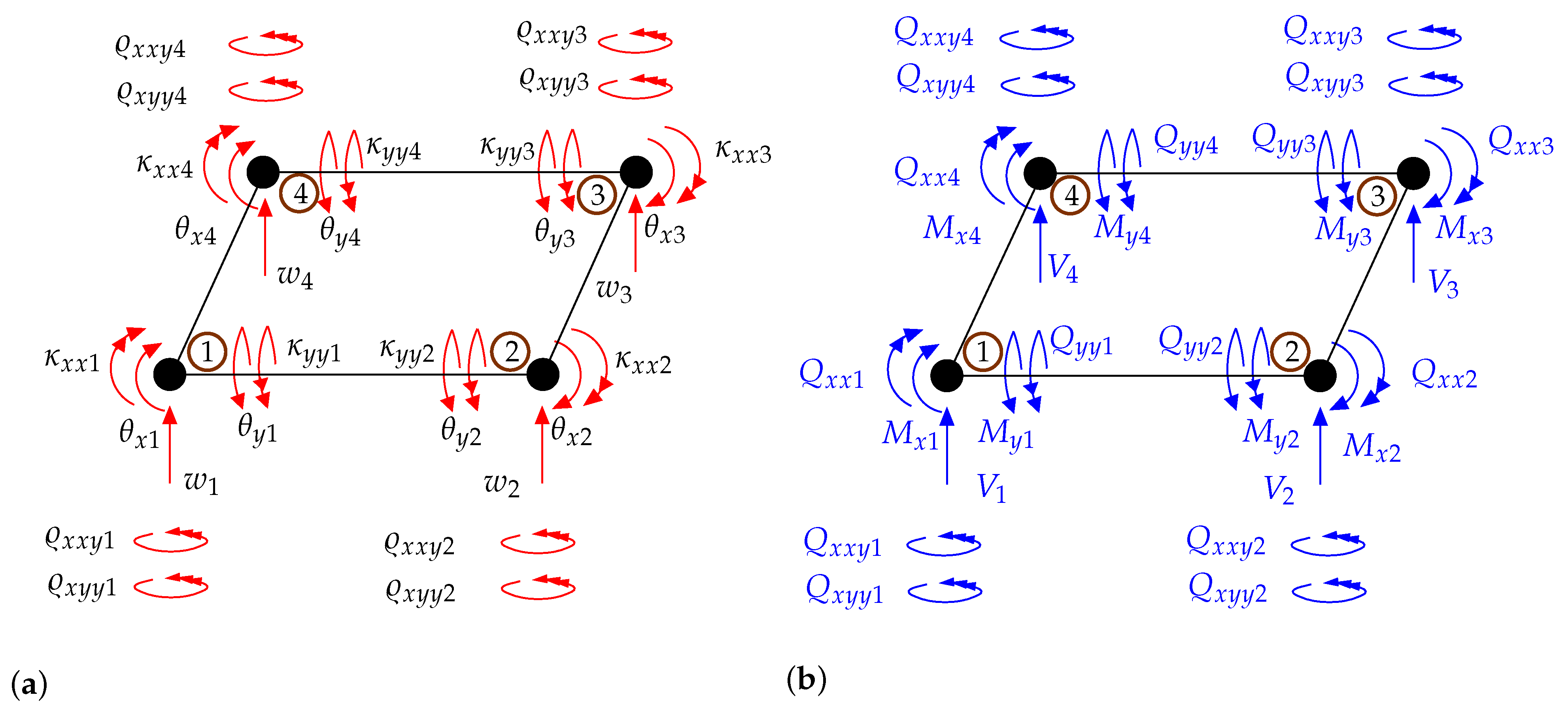
3.4. New 24-Dof Finite Element Formulation for Msgt-Based Kirchhoff Microplates

We develop the 24-DOF element from the 16-DOF BFS element in exactly the same manner the 20-DOF element is developed from the 12-DOF ACM element in Section 3.3. Herein the generalized displacements at the element nodes are prescribed as
1 . w = w 1 , θ x = θ x 1 , θ y = θ y 1 , κ x x = κ x x 1 , κ y y = κ y y 1 and κ x y = κ x y 1 , at at node 1 , 2 . w = w 2 , θ x = θ x 2 , θ y = θ y 2 , κ x x = κ x x 2 , κ y y = κ y y 2 and κ x y = κ x y 2 , at at node 2 , 3 . w = w 3 , θ x = θ x 3 , θ y = θ y 3 , κ x x = κ x x 3 , κ y y = κ y y 3 and κ x y = κ x y 3 , at at node 2 , 4 . w = w 4 , θ x = θ x 4 , θ y = θ y 4 , κ x x = κ x x 4 , κ y y = κ y y 4 and κ x y = κ x y 4 , at at node 4 ,
see Figure 7a. Similarly, the generalized nodal force resultants are prescribed as
1 . V = V 1 , M x = M x 1 , M y = M y 1 , Q x x = Q x x 1 , Q y y = Q y y 1 , and M x y = M x y 1 , at node 1 , 2 . V = V 2 , M x = M x 2 , M y = M y 2 , Q x x = Q x x 2 , Q y y = Q y y 2 , and M x y = M x y 2 , at node 2 , 3 . V = V 3 , M x = M x 3 , M y = M y 3 , Q x x = Q x x 3 , Q y y = Q y y 3 , and M x y = M x y 3 , at node 3 , 4 . V = V 4 , M x = M x 4 , M y = M y 4 , Q x x = Q x x 4 , Q y y = Q y y 4 , and M x y = M x y 4 , at node 4 ,
see Figure 7b. The element nodal displacement vector d and the element nodal force vector f are, respectively,
d T = w 1 θ x 1 θ y 1 κ x x 1 κ y y 1 κ x y 1 . . . w 4 θ x 4 θ y 4 κ x x 4 κ y y 4 κ x y 4 , f T = V 1 M x 1 M y 1 Q x x 1 Q y y 1 M x y 1 . . . V 4 M x 4 M y 4 Q x x 4 Q y y 4 M x y 4 ,
The displacement field w ( x , y ) within the element domain is then interpolated as
w ( x , y ) = N d = i = 1 n DOF j = 1 n nodes N i j d i j where N = N 1 1 N 2 1 N 3 1 N 4 1 N 5 1 N 6 1 . . . N 1 4 N 2 4 N 3 4 N 4 4 N 5 4 N 6 4
with number of DOFs per node is n DOF = 6 and number of nodes is n nodes = 4 . We propose a homogenous solution of the partial differential Equation (27) in the form
w ( x , y ) = a 1 + a 2 x + a 3 y + a 4 x 2 + a 5 x y + a 6 y 2 + a 7 x 3 + a 8 x 2 y + a 9 x y 2 + a 10 y 3 + a 11 x 3 y + a 12 x 2 y 2 + a 13 x y 3 + a 14 x 2 y 3 + a 15 x 3 y 2 + a 16 x 3 y 3 + a 17 sinh ( A x ) + a 18 cosh ( A x ) + a 19 sinh ( B y ) + a 20 cosh ( B y ) + a 21 sinh ( A x ) y + a 22 cosh ( A x ) y + a 23 sinh ( B y ) x + a 24 cosh ( B y ) x , with A = L d 1 / d 4 , B = W d 1 / d 4 ,
With similar hyperbolic sine and cosine terms, the equation above satisfies the homogeneous solution for Equation (27). Hence we also propose twenty-four shape functions as given in Equation (64). The first six of these shape functions (i.e., those for the first node) are shown in Figure 8. The remaining eighteen are symmetric with respect to two centroidal principal axes x ¯ and y ¯ around the geometric center of the element. The shape functions N 1 j , N 2 j , N 3 j , and N 6 j recover their classical counterparts in BFS element for j’th node whereas N 4 j and N 5 j vanish as length scale parameters tend to zero.
By changing of variables and the use of two-point Gaussian quadrature, the discrete representation for the element stiffness matrix k e similar to Section 3.3 is
k e = i = 1 2 j = 1 2 C N T E C C N + H N T E H H N det ( J ) Ω ( ξ 1 , ξ 2 ) | ξ 1 = ξ 1 ( i ) | ξ 2 = ξ 2 ( j ) ,
similar to the formulation in Section 3.3.
The 32-DOF finite element formulation variant derived from BFS and 24-DOF finite elements is given in Appendix F.

3.5. Conformity

Since the energy Equation (A12) in Appendix A involves terms with third derivatives of displacement w, C 2 -continuity is required for conformity. Herein, 20-DOF element is demonstrated and 24-, 28-, and 32-DOF versions behave similarly. Let us consider a rectangular element as depicted in Figure 9. For an element boundary AB, the C 2 -continuity would require displacements, rotations and curvatures to be uniquely defined in terms of the nodal degrees of freedoms, i.e., w, θ x , θ y , κ x and κ y at points A and B respectively (ten nodal variables). Similarly for an element boundary DA given in the same figure, these need to be defined by the same nodal variables at D and A. For the boundary along the element edge AD, where y is constant and zero
w = a 1 + a 2 x + a 4 x 2 + a 7 x 3 + a 13 sinh ( A x ) + a 14 cosh ( A x ) + a 16 + a 20 x , δ w δ x = a 2 + 2 a 4 x + 3 a 7 x 2 + a 13 A cosh ( A x ) + a 14 A sinh ( A x ) + a 20 , δ w δ y = a 3 + a 5 x + a 8 x 2 + a 11 x 3 + a 15 B + a 17 sinh ( A x ) + a 18 cosh ( A x ) + a 19 B x , δ 2 w δ x 2 = 2 a 4 + 6 a 7 x + A 2 a 13 sinh ( A x ) + A 2 a 14 cosh ( A x ) , δ 2 w δ y 2 = 2 a 6 + 2 a 9 x + B 2 a 16 + B 2 a 20 x ,
with 18 unkown constants that can not be defined by invoking 10 nodal displacement boundary conditions. Hence, just like its conventional counterpart [61], it is not possible to specify a polynomial set for the shape functions that ensure compatibility. The proposed elements are non-conforming elements whereas the convergence and numerical perfomance of the elements are investigated in Section 4. Cirak et al. [75,76] have overcome this problem in the context of classical Kirchfoff plates and shells by introducing a concept of triangular elements with subdivision surfaces where nonlocal interpolations are imposed on the subdivison elements, fully conforming to C 1 continuity requirements. The current contribution, however, shall be considered as a first step towards incorporating MSGT into Kirchhoff plates in the context of finite element method. In the subsequent part of the work, we also develop several elements with more degrees of freedom, particularly from the conforming Bogner-Fox-Schmit (BFS) element [59], in addition to adding more higher-order terms.

4. Representative Numerical Examples

In this section, the performances of the proposed 20-, 24-, 28-, and 32-DOF MSGT-based Kirchhoff plate elements are assessed under various boundary and loading conditions for different geometries. To this end, the finite element method outlined in Section 3.3 is implemented into our in-house finite element code that is developed via Matlab. First, the performance comparison is made between all the proposed elements. Then, we find the length scale parameters of gold based on the experiments of Espinosa et al. [60]. Four benchmark examples concerned with the assessment of the performance of the proposed element formulation with respect to mesh irregularity due to element size, mesh convergence, and response to various displacement boundary conditions are given. We then study the convergence of the numerical solutions to the approximate analytical solutions for a square and rectangular plate subjected to evenly distributed surface loads per the study of Movassagh and Moahmoodi [47]. Finally, several representative boundary value problems involving realistic MEMS switch geometries are investigated, and the results are compared with those obtained from the classical Kirchhoff plate theory. For all the problems, the number of elements and mesh size are chosen based on the studies given in Section 4.3.3.

4.1. Comparison

A basic comparison case study is performed by using a fixed-fixed plate with dimensions 20 μ m × 5 μ m × 1 μ m [32]. A concentrated midpoint load of F z = 1 mN is applied as shown in Figure 10. Therein, square elements are used with a mesh of 32 × 8 elements, i.e., with a mesh density of 1.6 elements/ μ m at the edges. The resulting deflection field is shown in Figure 11. The deflection profiles of the principal centroidal axes of the plates are depicted in Figure 12a,b respectively. The difference between the models constructed with 20-, 24-, 28-, and 32-DOF elements is insignificant -i.e., in the order of magnitude of 10 5 μ m and smaller than 0.2% of the total tip deflection-, and the deflection profile looks almost the same in Figure 12a. In Figure 12b the difference can be seen, along with a slight saddle effect that is expected due to Poisson effect [37].
Along with these results and similar results found for the forthcoming sections for the analysis of length scale parameters and assessment of element performance, only the results for the 20-DOF element are included for Section 4.2, Section 4.3 and Section 4.4.

4.2. Length Scale Parameters for Gold Microplates

Experiments in the study of Espinosa et al. [60] are modelled by microplates. The specimen dimensions and force-displacement values are given in Table 1, and the boundary conditions are shown in Figure 13. Force-displacement behavior is assumed as linear elastic and elastic parameters E and ν for Specimens 1 and 2 are assumed to be the same. The methodology is based on our previous study [32], i.e., for quantification of elastic modulus E and length scale parameter l, an error parameter Err is defined as the L 2 -norm of the residual vector, for the quantification of the best fit at which Err is minimum.
Err = ( w 1 w 1 exp ) 2 + ( w 2 w 2 exp ) 2 .
Herein w 1 and w 2 are the midpoint deflections predicted by higher order theories, w 1 exp and w 2 exp are the actual midpoint deflections from experiments for specimens 1 and 2. Err is evaluated for different values of E and l in order to find the minimum error. It is seen that the error function is minimum along the dark blue region in Figure 14. For bulk elastic modulus of gold i.e., E = 80 GPa, l 0 is found as 3.60 μ m.
Throughout the following numerical examples demonstrating element performance, these material parameters specific to gold are used. Those of epoxy are taken from the pioneering work of Lam et al. [28]. These are summarized in Table 2.

4.3. Assessment of Element Performance

The proposed MSGT-based Kirchhoff microplate elements can be used for rectangular elements similar to their classical counterparts. The results obtained with the developed MSGT-based Kirchhoff microplate are exactly the same with those with the ACM element, with vanishing length scale parameters. Although the ACM element passes the patch test, the usage area should be confined to rectangular meshes [61,77]. The proposed formulation shows similar performance to ACM element under distorted element geometries. In this regard, we confine ourselves to the investigation of the convergence behaviour upon mesh refinement and the element performance to irregular rectangular meshes. To this end, the convergence of the displacement field for a square block subjected to a point load is investigated for various boundary conditions, Additionally, the sensitivity of the displacement field to mesh irregularity under prescribed displacement/rotation field is investigated.

4.3.1. Microplate Response to Point Load

A 6 μ m × 6 μ m × 1 μ m microplate is subjected to a concentrated load of 1 mN applied at the centroid. The plate is double-cantilevered as depicted in Figure 15a. The problem is investigated with several meshes as shown in Figure 15 in order to assess its sensitivity to mesh irregularity. The corresponding deflection profiles are depicted in Figure 16a–d. In order to assess the difference in displacement fields, the midline deflections for the relevant nodes at x = 0 and y = 0 for the regular mesh and the irregular mesh given in Figure 16b are given in Figure 17a. The points correspond to the nodal displacement values along x = 0 and y = 0 . The problem is also solved with ACM element and similar midline deflections are indicated in Figure 17b. Therein, curves in between nodal values are interpolated with the element shape functions. It is seen that the deflections of the nodes for the regular and irregular meshes complement each other. The difference between centroidal deflections is smaller than 1% as seen in Figure 16, with the displacement fields aligned to a reasonably acceptable extent. In fact the average difference between the deformation results at the nodes is less than 1%, meaning it performs slightly better than ACM element does for midline deflections in both directions. Although it is suggested that the element size variation such as aspect ratio change to be minimum as a best practice, varying aspect ratios do not yield erroneous results at least up to some extent, regarding displacement results.

4.3.2. Microplate Response to Displacement and Rotation

In order to check the integrity of the formulation and consistency of the numerical implementation in x- and y-directions, the 6 μ m × 6 μ m × 1 μ m microplate is subjected to a unit displacement and rotation at two perpendicular edges, respectively, see Figure 18 (first column). Therein, the left edge is fixed along y-axis and the right edge is displaced 1 μ m in z-direction, see Figure 18a. Then, the same plate is subjected to a unit rotation (1 rad) about y-axis, see Figure 18b. The same procedure is repeated for the perpendicular direction in Figure 18c,d, respectively. The simulation is first carried out with 4 × 4 regular mesh (second column) and for an irregular mesh (third column). Although the proposed element is shown to be non-conforming in Section 3.5, the displacement fields obtained from the regular and irregular meshes are nearly identical. The average difference between the deformation results at the nodes is less than 1%, hence the performance is deemed to be satisfactory.

4.3.3. Mesh-Refinement and Convergence

The 6 μ m × 6 μ m × 1 μ m is now subjected to a concentrated midpoint load of 1 mN with both classical ACM elements and the proposed higher-order microplate element. The the boundary conditions are specified as (i) double-cantilevered (two opposite edges clamped, two opposite edges free) and (ii) wholly-cantilevered (all four sides clamped), see Figure 19 (first column). The displacement profile for these boundary conditions on a 4 × 4 mesh are given in Figure 19 (second column). The midpoint deflections versus element per edge results are depicted in Figure 20a–d, for the proposed element formulation and the ACM element, respectively. The proposed element formulation is converging slightly faster than the classical counterpart. The convergence behaviour of the proposed element upon mesh-refinement is satisfactory for rectangular meshes given that the differences between the maximum displacement for consequent mesh refinements are less than 0.1%.

4.3.4. Square Microplate Subjected to Different Boundary Conditions

A 20 μ m × 20 μ m × 1 μ m microplate subjected to a point load is analyzed under various boundary conditions with the classical ACM plate element and the proposed MSGT-based microplate element formulations, respectively. Four different boundary conditions are considered, see Figure 21: (a) CFCF, (b) CFFF, (c) CCFC and (d) CCFC. The boundary conditions are abbreviated by "C" for clamped ends and by "F" for free ends. In the example (a) a centroidal, (b) midpoint of the free edge, (c) centroidal and (d) midpoint of the free edge, are subjected to point load, respectively. The domain is discretized with 20 × 20 elements. The results obtained from the classical ACM plate finite element and the porposed finite element formulation are visualized in Figure 21. In order to study the difference between the deformation patterns obtained from the classical and MSGT-based Kirchhoff theory, the contour plots are normalized with respect to the peak values. The numerical results show that, not only the maximum deflections but also the deformation patterns change significantly by considering the size effect in terms of the modified strain gradient theory.
It is seen in Figure 22 that the MSGT approaches asymptotically to classical theory as the thickness, which is related to structural length scale, increases. With the assumed length-width-thickness (aspect) ratio of 20:20:1 for gold microstructures, the error of using classical theory with macroscopic material parameters vary with boundary conditions. It still seems to be more than 10% if thickness is reduced below ca. 40 μ m at best case. This error increases with decreasing plate thickness - it becomes more than 25% if the relevant thickness is taken smaller than ca. 25 μ m at best case. It is seen that for the particular cases with 20 μ m × 20 μ m × 1 μ m microplate, the size effect yields deflections in the range of 0.3–0.5% of the deflections that are found with classical theory.

4.4. Benchmark Example: Rectangular Microplates Subjected to Evenly Distributed Load

Three benchmark examples, which are analytically solved by Movassagh and Mahmoodi [47] using extended Kantarovich method (EKM), are numerically reproduced with the proposed higher-order microplate elements. The boundary conditions and the dimensions in terms of the length scale parameters l = l 0 = l 1 = l 2 are depicted in Figure 23a–c. A distributed load of 1 kN/m 2 is applied in all three cases. Therein, the material parameters specific to epoxy are used [28], see Table 2. The normalized midpoint deflections ( w / l ) versus number of elements per length results are depicted in Figure 24a–c. The numerical results recover the analytical solution of Movassagh and Mahmoodi upon mesh refinement for all three cases. The difference between the results for consequent three refinements are less than 0.05%.

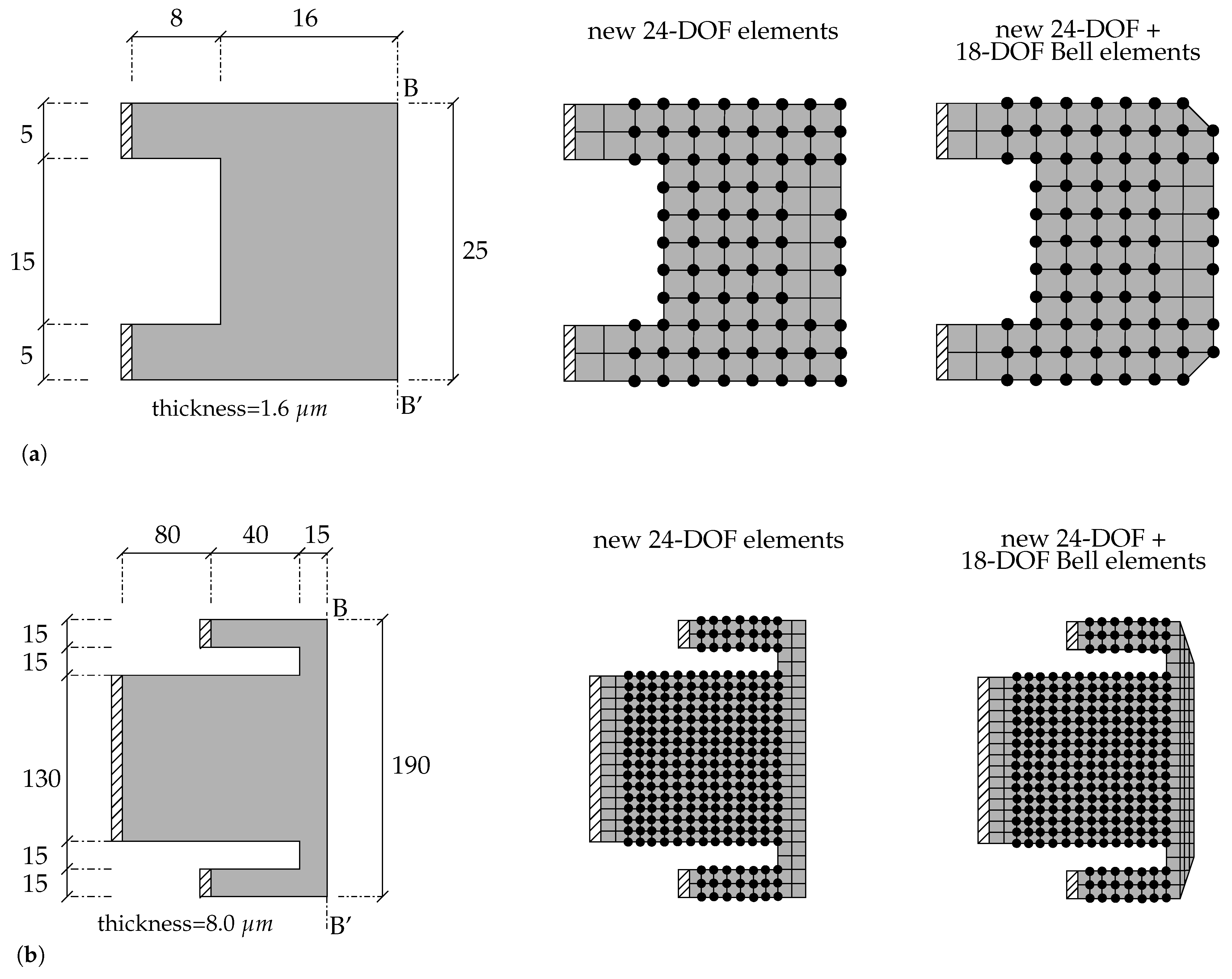
4.5. Analysis of Realistic Mems Switches with 20-Dof Elements

In this example, we consider three real MEMS switch structures from Patel and Rebeiz [66] and Stefanini et al. [65], respectively. The chamfers of the plates and tethers are ignored in this section. The geometry and the boundary conditions are depicted in Figure 25. Stefanini et al. [65] discusses an actuation electrode and the corresponding MEMS structure (see Figure 25a) to transfer the majority of the electrostatic force to the contact force, i.e.,
F c = 0.64 F e F r
where F c is the contact force, F r is the release force, and F e is the electrostatic force. Therein, F c = 34.7 μ N, F r = 15.5 μ N, and hence the electrostatic force is found as F e = 77.2 μ N. This force is equally distributed to the nodes that are electrostatically actuated, see Figure 25a. The deflection of the plate should be equal to the clearance of 0.3 μ m for contact condition. The electrostatic loads are applied to the structures and the deflected shapes, which are obtained from classical and the MSGT-based Kirchhoff plate theory, are shown in Figure 26. The analyses reveal, as expected, considerably softer response with the classical theory, see Figure 26a and Figure 27a. The normalized deflection curves that demonstrate the difference between the deflection profiles are given in Figure 28a. With MSGT and with the length scale parameters l 0 = l 1 = l 2 = 0.69 μ m, the contact condition can be achieved, as seen from the same figures. The study of Patel and Rebeiz [66] focuses on two MEMS switches (see Figure 25b,c) for which the electrostatic force for contact condition is given between 2.5–3.5 mN. It is hence assumed that an average electrostatic force of 3.0 mN is applied. This force is again equally distributed to the relevant nodes, see Figure 25b–c. The clearance in the design of these MEMS switches is 0.55 μ m. As in the example above, a considerably larger tip deflection is found with the classical theory. The analyses with MSGT-based Kirchhoff plate yield the required deflection, see Figure 26b,c and Figure 27b,c. Similarly, Figure 28b,c indicate the normalized deflection curves that demonstrates the difference between the deflection profiles. The corresponding length scale parameters that are adopted for these MEMS switches are l 0 = l 1 = l 2 = 2.87 μ m and l 0 = l 1 = l 2 =‘3.16 μ m respectively (see parts (b) and (c) of Figure 26, Figure 27 and Figure 28. In these three examples one can observe that higher-order theories significantly improve the analysis results. It is also revealed that complex planar structures that could not be reduced to beam structures and could not be modelled with MSGT previously, examples of which are given in Figure 25a,b, can now be designed and analyzed more effectively making use of the new MSGT plate elements.
The MEMS community traditionally use higher elasticity parameters such as Young’s modulus μ and shear modulus μ . This choice, for uniform thickness and under pure bending deformations leads to satisfactory results in line with the modified couple stress theory (MCST). This is mainly due to the fact that, MCST, when applied to Kirchhoff plate theory, leads to the same differential equation as the classical counterpart, where the nonlocal effects are merely reflected to the material parameters. In order to assess the difference between two theories, we depict the normalized tip deflections corresponding to each switch structure in Figure 28. The normalized tip deflections of the classical and the MCST-based Kirchhoff theory will lead to equivalent result. The idea here is to show, how the deflection pattern changes as we switch to the MSGT-based Kircchhoff plate theory from the classical counterpart or the MCST-based Kirchhoff plate theory. As seen from, Figure 28, for cantilever geometries, where the bending governs the deformation, normalized results overlap. However, for the second geometry, where highly complex local and nonlocal deformations exist due to the complex geometry and boundary conditions, the normalized deflection patterns are quite dissimilar, revealing the necessity for the MSGT-based Kirchhoff plate theory.

4.6. Analysis of Realistic Mems Switches with 24-Dof Elements

We consider the two real MEMS switch structures from Stefanini et al. [65] and Patel and Rebeiz [66] that had been investigated in the previous section. In this section, chamfers are added, making the geometric models more realistic considering their original shapes in respective studies. The geometry and the boundary conditions are depicted in Figure 29.
We solve the problems by making use of the rectangular mesh (figures in the middle in Figure 25) as well as with a mesh consisting of 18-DOF Bell triangular and 24-DOF rectangular elements (figures on the right in Figure 25). For the triangular-rectangular mesh, very few 18-DOF Bell elements are used as seen in the relevant figure. Herein, in determining the higher-order stiffness matrix for the 18-DOF Bell element, Equation (58) is used that incorporate the higher-order d 1 d 6 terms and hence the length scale parameters l 0 , l 1 , and l 2 for the readily available classical Bell triangular element with the explicitly defined shape functions [78]. The length scale parameters are chosen as found in Section 4.2. The mix of rectangular-triangular elements yield the deflection fields as given in Figure 30. The deflection profile of the end tips are also given in Figure 31 for the rectangular mesh in the first study and the mix of rectangular-triangular elements. The average difference of all data points when compared with the purely rectangular mesh is ca. 0.2% for the case in Stefanini et al. [65] and ca. 0.02% for the case in Patel and Rebeiz [66]. It can then be concluded that the use of triangular Bell elements especially in the truncated parts of the microplates does not result in a considerable difference in the analyses when used with the same length scale parameters.

5. Conclusions

In this paper, we presented novel MSGT-based element formulations for Kirchhoff plate theory-based on the variational principle dictating the minimum potential energy. Finite element discretization is implemented based on this framework and relevant codes are developed. Herein, 2 × 2 Gaussian quadrature is implemented. Despite being non-conforming elements and only applicable to rectangular meshes similar to the original classical plate elements, it is demonstrated that the new elements yield expected results in various numerical examples. It is explicitly demonstrated that the convergence and aspect ratio test performances of the proposed elements are equivalent the classical elements. The numerical problems investigated clearly show that using the classical plate theory in predicting microplate behavior results in significant errors, especially if the thickness of the structures are smaller than 40 μ m.
In the future, discrete techniques, isogeometric methods, or similar will be utilized to come up with a conforming higher-order element applicable to general quadrilaterals, satisfying C 2 -continuity requirement. However, it is also worth mentioning that many, if not most, of the MEMS-NEMS plate structures can be modelled with only rectangular elements, similar to the ones modelled and analyzed in this study.
All simulations are carried out on a standard Laptop with Intel I7 processor having 8 × 2.4 GHz cores and 8 GB Ram, without any parallelization, requiring several minutes of computation time for the most demanding simulation. Computational timing benchmarks for the analyses mentioned under Section 4.1 reveal that analysis with MSGT with the newly developed elements takes up to approximately 2 min, 14 × longer than classical analyses which takes less than 10 s, ceteris paribus. This is in fact why 2 × 2 Gaussian quadrature method is adopted, which decreases the computational duration ratio up to 6 at most, when compared to the classical theory, again ceteris paribus, yielding a computational duration of less than 1 min. This computational time ratio of approximately 6 is found in other analyses within this study as well. It is noted however, most MEMS-NEMS structures can be modelled with very small number of nodes and elements than macrostructures, hence the increase in the computational time can be tolerated with the state of the art CPUs and parallelization techniques.

Author Contributions

Conceptualization, H.D.; methodology, M.K. and H.D.; software, M.K.; validation, M.K. and H.D.; formal analysis, M.K. and H.D.; investigation, M.K. and H.D.; resources, M.K. and H.D.; writing—original draft preparation, M.K.; writing—review and editing, H.D.; visualization, M.K. and H.D.; supervision, H.D.; funding acquisition, H.D. All authors have read and agreed to the published version of the manuscript.

Funding

This research was funded by TUBITAK 1001 under grant number 116M258.

Institutional Review Board Statement

Not applicable.

Informed Consent Statement

Not applicable.

Conflicts of Interest

The authors declare no conflict of interest.

Appendix A. Derivation of Euler-Lagrange Equations of Msgt-Based for Kirchhoff Microplates

The internal energy equation with the strain and stress metrics of MSGT becomes:
Π i n t = 1 2 B σ : ε + p · ε + τ     η 1 + m · χ d V = 1 2 B ( σ i j ε i j + p i γ i + τ i j k η i j k + m i j χ i j ) d V
where γ is expressed as the dilation gradient vector as
γ = ( compact notation ) γ i = ε m m , i ( indicial notation )
in compact notation and indicial notation respectively. Then, for a general plate structure,
δ Π i n t = B ( σ x x δ ε x x + 2 σ x y δ ε x y + σ y y δ ε y y + p x δ γ x + p y δ γ y + p z δ γ z + τ x x x 1 δ η x x x 1 + 3 τ x x y 1 δ η x x y 1 + 3 τ x x z 1 δ η x x z 1 + 3 τ x y y 1 δ η x y y 1 + τ y y y 1 δ η y y y 1 + 3 τ y y z 1 δ η y y z 1 + 3 τ x z z 1 δ η x z z 1 + 3 τ y z z 1 δ η y z z 1 + τ z z z 1 δ η z z z 1 + 6 τ x y z 1 δ η x y z 1 + m x x δ χ x x + 2 m x y δ χ x y + m y y δ χ y y ) d V .
In order to evaluate above, the terms are identified. Using the displacement field of a Kirchhoff plate given in Equation (12), the classical strain terms can be found as:
ε x x = z w , x x , ε y y = z w , y y , ε x y = z w , x y .
The dilatation gradient terms can then be derived as:
γ x = ε m m , x = z w , x x x + w , y y x , γ y = ε m m , y = z w , y x x + w , y y y , γ z = ε m m , z = 2 w = w , x x + w , y y .
The indicial expression for deviatoric stretch gradient terms ( η 1 ) is:
η i j k 1 = η i j k S 1 5 δ i j η m m k S + δ j k η m m i S δ k i η m m j S where η i j k S = 1 3 u i , j k + u j , k i + u k , i j ,
and where δ i j is the Kronecker’s delta. After several steps, the terms of the nonlocal deviatoric stretch gradient tensor are derived as
η x x x 1 z 5 2 3 w x 3 + 3 3 w y 2 x , η x x y 1 z 5 4 3 w x 2 y + 3 w y 3 , η x y y 1 z 5 4 3 w x y 2 + 3 w x 3 , η y y y 1 z 5 2 3 w y 3 + 3 3 w x 2 y , η x x z 1 1 15 4 2 w x 3 + 2 w y 2 , η x z z 1 z 5 3 w x 3 + 3 w x y 2 , η y z z 1 z 5 3 w y 3 + 3 w y x 2 , η z z z 1 1 5 2 w x 2 + 2 w y 2 η x y z 1 1 3 2 w x y ,
with
η x y x 1 = η y x x 1 = η x x y 1 , η x z x 1 = η z x x 1 = η x x z 1 , η y x y 1 = η y y x 1 = η x y y 1 , η z x z 1 = η z z x 1 = η x z z 1 , η z y z 1 = η z z y 1 = η y z z 1 , η y z x 1 = η z x y 1 = η z y x 1 = η y x z 1 = η x z y 1 = η x y z 1 .
The curvature or the rotation gradient terms in indicial notation are
χ i j = 1 4 e i m n u n , m j + e j m n u n , m i , where
e i j k is the permutation symbol. After some manipulations, the components of the curvature tensor read
χ x x = 2 w x y , χ y y = 2 w x y , χ x y = 1 2 2 w y 2 2 w x 2 , with χ z z = χ z x = χ x z = χ y z = χ z y = 0 .
Taking the variations of above expressions and multiplying with their stress conjugates as appearing in Equation (A3), the following are acquired:
σ x x δ ε x x = σ x x z δ w , x x , τ x x x 1 δ η x x x 1 = 2 5 z τ x x x 1 δ w , x x x + 3 5 z τ x x x 1 δ w , x y y , 2 σ x y δ ε x y = 2 σ x y z δ w , x y , 3 τ x x y 1 δ η x x y 1 = 12 5 z τ x x y 1 δ w , x x y + 3 5 z τ x x y 1 δ w , y y y , σ y y δ ε y y = σ y y z δ w , y y , 3 τ x x z 1 δ η x x z 1 = 4 5 τ x x z 1 δ w , x x + 1 5 τ x x z 1 δ w , y y , p x δ γ x = p x z δ w , x x x p x z δ w , x y y , 3 τ x y y 1 δ η x y y 1 = 12 5 z τ x y y 1 δ w , x y y + 3 5 z τ x y y 1 δ w , x x x , p y δ γ y = p y z δ w , y y y p y z δ w , x x y , τ y y y 1 δ η y y y 1 = 3 5 z τ y y y 1 δ w , x x y 1 5 z τ y y y 1 δ w , y y y , p z δ γ z = p z δ w , x x p z δ w , y y , 3 τ y y z 1 δ η y y z 1 = 1 5 τ y z z 1 δ w , x x 4 5 τ y y z 1 δ w , y y , m x x δ χ x x = m x x δ w , x y , τ x z z 1 δ η x z z 1 = 3 5 z τ x z z 1 δ w , x x x 3 5 z τ x z z 1 δ w , x y y , 2 m x y δ χ x y = m x y δ w , y y m x y δ w , x x , τ y z z 1 δ η y z z 1 = 3 5 z τ y z z 1 δ w , x x y 1 5 z τ y z z 1 δ w , y y y , m y y δ χ y y = m y y δ w , x y , τ z z z 1 δ η z z z 1 = 1 5 τ z z z 1 δ w , x x 1 5 τ z z z 1 δ w , y y , 6 τ x y z 1 δ η x y z 1 = 2 τ x y z 1 δ w , x y .
Given the above expressions, Equation (A3) can now we written as:
δ Π i n t = B M x x δ w , x x + M x y δ w , x y + M y y δ w , y y + Q x x x δ w , x x x + Q x x y δ w , x x y + Q x y y δ w , x y y + Q y y y δ w , y y y d A .
where B is 2D domain of the mid-plane of the plate bounded by a piecewise smooth curve Γ . Then
M x x = h / 2 h / 2 σ x x z p z 4 5 τ x x z 1 + 1 5 τ y y z 1 + 1 5 τ z z z 1 m x y d z
M x y = h / 2 h / 2 2 σ x y z 2 τ x y z 1 + m x x m y y d z
M y y = h / 2 h / 2 σ y y z p z + 1 5 τ x x z 1 4 5 τ y y z 1 + 1 5 τ z z z 1 + m x y d z
Q x x x = h / 2 h / 2 z 5 5 p x 2 τ x x x 1 + 3 τ x y y 1 + 3 τ x z z 1 d z
Q x x y = h / 2 h / 2 z 5 5 p x + 2 τ x x x 1 12 τ x y y 1 + 3 τ x z z 1 d z
Q x y y = h / 2 h / 2 z 5 5 p y 12 τ x x y 1 + 3 τ y y y 1 + 3 τ y z z 1 d z
Q y y y = h / 2 h / 2 z 5 5 p y + 3 τ x x y 1 2 τ y y y 1 + 3 τ y z z 1 d z
Inserting the stress terms, stress resultant terms read
M x x = μ h h 2 6 ( 1 ν ) + 2 μ l 0 2 + 8 15 μ l 1 2 + μ l 2 2 w , x x + μ h ν h 2 6 ( 1 ν ) + 2 μ l 0 2 2 15 μ l 1 2 μ l 2 2 w , y y ,
M x y = μ h h 2 3 + 4 3 μ l 1 2 + 4 μ l 2 2 w , x y ,
M y y = μ h h 2 6 ( 1 ν ) + 2 μ l 0 2 2 15 μ l 1 2 + μ l 2 2 w , x x + μ h ν h 2 6 ( 1 ν ) + 2 μ l 0 2 + 8 15 μ l 1 2 μ l 2 2 w , y y ,
Q x x x = μ h 3 6 l 0 2 + 2 5 l 1 2 w , x x x + μ h 3 6 l 0 2 3 5 l 1 2 w , x y y ,
Q x x y = μ h 3 6 l 0 2 + 12 5 l 1 2 w , x x y + μ h 3 6 l 0 2 3 5 l 1 2 w , y y y ,
Q x y y = μ h 3 6 l 0 2 3 5 l 1 2 w , x x x + μ h 3 6 l 0 2 + 12 5 l 1 2 w , x y y ,
Q y y y = μ h 3 6 l 0 2 3 5 l 1 2 w , x x y + μ h 3 6 l 0 2 + 2 5 l 1 2 w , y y y .
Now, using the divergence theorem for Equation (A12) and minimum potential energy principle with
Π e x t = B q ( x , y ) δ w d A
we obtain the Euler-Lagrange equation governing the minimization principle
M x x , x x + M x y , x y + M y y , y y Q x x x , x x x Q x x y , x x y Q x y y , x y y Q y y y , y y y = q ( x , y ) .
Insertion of Equations (A20)–(A26) into (A28) leads to the Equation (27).

Appendix B. Shape Functions for Acm Element Based on Classical Kirchhoff Plate Theory

The first three elements of ACM shape functions N 1 corresponding to the first node for classical theory, which are shown in Figure 3, are as given as:
N 1 1 = 2 ξ 1 3 ξ 2 + 2 ξ 1 3 + 3 ξ 1 2 ξ 2 3 ξ 1 2 2 ξ 1 ξ 2 3 + 2 ξ 2 3 + 3 ξ 1 ξ 2 2 3 ξ 2 2 ξ 1 ξ 2 + 1 , N 2 1 = ξ 1 ξ 2 3 + ξ 2 3 + 2 ξ 1 ξ 2 2 2 ξ 2 2 ξ 1 ξ 2 + ξ 2 , N 3 1 = ξ 1 3 ξ 2 ξ 1 3 2 ξ 1 2 ξ 2 + 2 ξ 1 2 + ξ 1 ξ 2 ξ 1 with ξ 1 = x / L and ξ 2 = y / W .

Appendix C. Shape Functions of the Proposed Element for Msgt-Based Kirchhoff Microplates

The first five elements of the shape function N for MSGT, which are shown in Figure 6, are as given below.
N 1 1 = ( 144 A sinh ( A ξ 1 ) 288 ξ 2 288 cosh ( A ξ 1 ) 288 cosh ( B ξ 2 ) 288 ξ 1
+ 144 B sinh ( B ξ 2 ) + 576 ξ 1 ξ 2 + 288 ξ 2 cosh ( A ξ 1 ) + 288 ξ 1 cosh ( B ξ 2 ) 144 A sinh ( A )
144 B sinh ( B ) 96 A 2 ξ 1 96 B 2 ξ 2 + 288 ξ 1 cosh ( A ) + 48 B 2 cosh ( A ξ 1 )
+ 288 ξ 1 cosh ( B ) + 288 ξ 2 cosh ( A ) + 48 A 2 cosh ( B ξ 2 ) + 288 ξ 2 cosh ( B ) + 288 cosh ( A ξ 1 ) cosh ( A )
+ 288 cosh ( A ξ 1 ) cosh ( B ) + 288 cosh ( B ξ 2 ) cosh ( A ) + 288 cosh ( B ξ 2 ) cosh ( B )
288 sinh ( A ξ 1 ) sinh ( A ) 288 sinh ( B ξ 2 ) sinh ( B ) + 48 A 2
16 A 2 B 2 + 48 B 2 + 96 A 2 cosh ( A ) 48 A 2 cosh ( B ) 48 B 2 cosh ( A )
+ 96 B 2 cosh ( B ) 12 A 3 sinh ( A ) 12 B 3 sinh ( B ) + 144 A 2 ξ 1 2 96 A 2 ξ 1 3
+ 144 B 2 ξ 2 2 96 B 2 ξ 2 3 + 288 ξ 2 sinh ( A ξ 1 ) sinh ( A ) + 288 ξ 1 sinh ( B ξ 2 ) sinh ( B )
+ 24 A 2 B 2 ξ 1 + 24 A 2 B 2 ξ 2 48 A 2 ξ 1 cosh ( A ) + 96 A 2 ξ 1 cosh ( B ) + 96 B 2 ξ 2 cosh ( A )
48 B 2 ξ 2 cosh ( B ) 48 B 2 cosh ( A ξ 1 ) cosh ( A ) 288 ξ 1 cosh ( A ) cosh ( B )
+ 96 B 2 cosh ( A ξ 1 ) cosh ( B ) + 96 A 2 cosh ( B ξ 2 ) cosh ( A ) 288 ξ 2 cosh ( A ) cosh ( B )
48 A 2 cosh ( B ξ 2 ) cosh ( B ) 288 cosh ( A ξ 1 ) cosh ( A ) cosh ( B )
12 A 3 ξ 1 sinh ( A ) 12 B 3 ξ 2 sinh ( B ) 12 B 3 cosh ( A ξ 1 ) sinh ( B ) 12 A 3 cosh ( B ξ 2 ) sinh ( A )
+ 48 B 2 sinh ( A ξ 1 ) sinh ( A ) + 48 A 2 sinh ( B ξ 2 ) sinh ( B )
+ 288 sinh ( B ξ 2 ) cosh ( A ) sinh ( B ) 144 A 2 ξ 1 2 ξ 2 + 96 A 2 ξ 1 3 ξ 2 144 B 2 ξ 1 ξ 2 2
+ 96 B 2 ξ 1 ξ 2 3 32 A 2 B 2 cosh ( A ) 32 A 2 B 2 cosh ( B ) 96 A 2 cosh ( A ) cosh ( B )
96 B 2 cosh ( A ) cosh ( B ) + 4 A 3 B 2 sinh ( A ) + 4 A 2 B 3 sinh ( B ) + 12 A 3 cosh ( B ) sinh ( A )
+ 12 B 3 cosh ( A ) sinh ( B ) 24 A 2 B 2 ξ 1 2 + 16 A 2 B 2 ξ 1 3 24 A 2 B 2 ξ 2 2
+ 16 A 2 B 2 ξ 2 3 144 A 2 ξ 1 2 cosh ( A ) + 96 A 2 ξ 1 3 cosh ( A ) 144 A 2 ξ 1 2 cosh ( B ) + 96 A 2 ξ 1 3 cosh ( B )
144 B 2 ξ 2 2 cosh ( A ) + 96 B 2 ξ 2 3 cosh ( A ) 144 B 2 ξ 2 2 cosh ( B ) + 96 B 2 ξ 2 3 cosh ( B ) + 72 A 3 ξ 1 2 sinh ( A )
48 A 3 ξ 1 3 sinh ( A ) + 72 B 3 ξ 2 2 sinh ( B ) 48 B 3 ξ 2 3 sinh ( B ) 144 A ξ 2 sinh ( A ξ 1 ) 144 B ξ 1 sinh ( B ξ 2 )
24 A B 2 sinh ( A ξ 1 ) 144 A ξ 2 sinh ( A ) 144 B ξ 1 sinh ( B ) 144 A cosh ( A ξ 1 ) sinh ( A )
+ 144 A sinh ( A ξ 1 ) cosh ( A ) 24 A 2 B sinh ( B ξ 2 ) 144 A sinh ( A ξ 1 ) cosh ( B )
288 B cosh ( A ξ 1 ) sinh ( B ) 288 A cosh ( B ξ 2 ) sinh ( A ) 144 B sinh ( B ξ 2 ) cosh ( A )
144 B cosh ( B ξ 2 ) sinh ( B ) + 144 B sinh ( B ξ 2 ) cosh ( B ) + 48 A 2 ξ 1 ξ 2
+ 48 B 2 ξ 1 ξ 2 576 ξ 1 ξ 2 cosh ( A ) 48 A 2 ξ 1 cosh ( B ξ 2 ) 48 B 2 ξ 2 cosh ( A ξ 1 ) 576 ξ 1 ξ 2 cosh ( B )
288 ξ 2 cosh ( A ξ 1 ) cosh ( A ) 288 ξ 1 cosh ( B ξ 2 ) cosh ( A ) 288 ξ 2 cosh ( A ξ 1 ) cosh ( B )
288 ξ 1 cosh ( B ξ 2 ) cosh ( B ) + 72 A B 2 sinh ( A ) + 72 A 2 B sinh ( B ) + 144 A cosh ( B ) sinh ( A )
+ 144 B cosh ( A ) sinh ( B ) A 3 B 3 sinh ( A ) sinh ( B ) + 24 A 2 B 2 ξ 1 2 cosh ( A )
16 A 2 B 2 ξ 1 3 cosh ( A ) 48 A 2 B 2 ξ 1 2 cosh ( B ) + 32 A 2 B 2 ξ 1 3 cosh ( B ) 48 A 2 B 2 ξ 2 2 cosh ( A ) + 32 A 2 B 2 ξ 2 3 cosh ( A )
+ 24 A 2 B 2 ξ 2 2 cosh ( B ) 16 A 2 B 2 ξ 2 3 cosh ( B ) + 144 A 2 ξ 1 2 cosh ( A ) cosh ( B ) 96 A 2 ξ 1 3 cosh ( A ) cosh ( B )
+ 144 A B sinh ( A ξ 1 ) sinh ( B ) + 144 B 2 ξ 2 2 cosh ( A ) cosh ( B ) 96 B 2 ξ 2 3 cosh ( A ) cosh ( B )
+ 144 A B sinh ( B ξ 2 ) sinh ( A ) 12 A 3 B 2 ξ 1 2 sinh ( A ) + 8 A 3 B 2 ξ 1 3 sinh ( A ) + 6 A 2 B 3 ξ 1 2 sinh ( B )
4 A 2 B 3 ξ 1 3 sinh ( B ) + 6 A 3 B 2 ξ 2 2 sinh ( A ) 4 A 3 B 2 ξ 2 3 sinh ( A ) 12 A 2 B 3 ξ 2 2 sinh ( B ) + 8 A 2 B 3 ξ 2 3 sinh ( B )
72 A 3 ξ 1 2 cosh ( B ) sinh ( A ) + 48 A 3 ξ 1 3 cosh ( B ) sinh ( A ) 72 B 3 ξ 2 2 cosh ( A ) sinh ( B )
+ 48 B 3 ξ 2 3 cosh ( A ) sinh ( B ) + 288 A ξ 1 ξ 2 sinh ( A ) + 24 A B 2 ξ 2 sinh ( A ξ 1 ) + 24 A 2 B ξ 1 sinh ( B ξ 2 )
+ 288 B ξ 1 ξ 2 sinh ( B ) + 144 A ξ 2 cosh ( A ξ 1 ) sinh ( A ) 144 A ξ 2 sinh ( A ξ 1 ) cosh ( A )
+ 288 A ξ 1 cosh ( B ξ 2 ) sinh ( A ) + 144 A ξ 2 sinh ( A ξ 1 ) cosh ( B ) + 144 B ξ 1 sinh ( B ξ 2 ) cosh ( A )
+ 288 B ξ 2 cosh ( A ξ 1 ) sinh ( B ) + 144 B ξ 1 cosh ( B ξ 2 ) sinh ( B ) 144 B ξ 1 sinh ( B ξ 2 ) cosh ( B )
288 A B sinh ( A ) sinh ( B ) 48 A B 2 ξ 1 sinh ( A ) 120 A 2 B ξ 1 sinh ( B ) 120 A B 2 ξ 2 sinh ( A )
48 A 2 B ξ 2 sinh ( B ) + 24 A B 2 cosh ( A ξ 1 ) sinh ( A ) 24 A B 2 sinh ( A ξ 1 ) cosh ( A )
48 A B 2 sinh ( A ξ 1 ) cosh ( B ) + 144 B ξ 1 cosh ( A ) sinh ( B ) + 144 A ξ 2 cosh ( B ) sinh ( A )
48 A 2 B sinh ( B ξ 2 ) cosh ( A ) + 144 A cosh ( A ξ 1 ) cosh ( B ) sinh ( A )
144 A sinh ( A ξ 1 ) cosh ( A ) cosh ( B ) + 24 A 2 B cosh ( B ξ 2 ) sinh ( B ) 24 A 2 B sinh ( B ξ 2 ) cosh ( B )
+ 288 B cosh ( A ξ 1 ) cosh ( A ) sinh ( B ) + 288 A cosh ( B ξ 2 ) cosh ( B ) sinh ( A )
+ 144 B cosh ( B ξ 2 ) cosh ( A ) sinh ( B ) 144 B sinh ( B ξ 2 ) cosh ( A ) cosh ( B ) + 6 A B 3 sinh ( A ξ 1 ) sinh ( B )
+ 6 A 3 B sinh ( B ξ 2 ) sinh ( A ) 32 A 2 B 2 ξ 1 ξ 2 48 A 2 ξ 1 ξ 2 cosh ( A ) 48 A 2 ξ 1 ξ 2 cosh ( B )
48 B 2 ξ 1 ξ 2 cosh ( A ) 48 B 2 ξ 1 ξ 2 cosh ( B ) 96 A 2 ξ 1 cosh ( B ξ 2 ) cosh ( A ) + 48 B 2 ξ 2 cosh ( A ξ 1 ) cosh ( A )
+ 576 ξ 1 ξ 2 cosh ( A ) cosh ( B ) + 48 A 2 ξ 1 cosh ( B ξ 2 ) cosh ( B ) 96 B 2 ξ 2 cosh ( A ξ 1 ) cosh ( B )
288 B sinh ( A ξ 1 ) sinh ( A ) sinh ( B ) + 288 ξ 2 cosh ( A ξ 1 ) cosh ( A ) cosh ( B )
288 A sinh ( B ξ 2 ) sinh ( A ) sinh ( B ) + 24 A 3 ξ 1 ξ 2 sinh ( A ) + 24 B 3 ξ 1 ξ 2 sinh ( B ) + 12 A 3 ξ 1 cosh ( B ξ 2 ) sinh ( A )
+ 288 ξ 1 cosh ( B ξ 2 ) cosh ( A ) cosh ( B ) + 144 A B 2 cosh ( B ) sinh ( A ) + 144 A 2 B cosh ( A ) sinh ( B )
+ 288 sinh ( A ξ 1 ) cosh ( B ) sinh ( A ) 288 cosh ( B ξ 2 ) cosh ( A ) cosh ( B ) + 12 B 3 ξ 2 cosh ( A ξ 1 ) sinh ( B )
48 B 2 ξ 2 sinh ( A ξ 1 ) sinh ( A ) 18 A B 3 sinh ( A ) sinh ( B ) 18 A 3 B sinh ( A ) sinh ( B )
48 A 2 ξ 1 sinh ( B ξ 2 ) sinh ( B ) 288 ξ 2 sinh ( A ξ 1 ) cosh ( B ) sinh ( A )
288 ξ 1 sinh ( B ξ 2 ) cosh ( A ) sinh ( B ) + 24 A 2 B 2 ξ 1 cosh ( A ) + 48 A 2 B 2 ξ 1 cosh ( B ) + 48 A 2 B 2 ξ 2 cosh ( A )
+ 24 A 2 B 2 ξ 2 cosh ( B ) + 48 A 2 ξ 1 cosh ( A ) cosh ( B ) + 48 B 2 ξ 2 cosh ( A ) cosh ( B )
96 B 2 cosh ( A ξ 1 ) cosh ( A ) cosh ( B ) 96 A 2 cosh ( B ξ 2 ) cosh ( A ) cosh ( B ) + 144 A 2 B ξ 1 2 sinh ( B )
96 A 2 B ξ 1 3 sinh ( B ) 6 A 2 B 3 ξ 1 sinh ( B ) + 144 A B 2 ξ 2 2 sinh ( A ) 96 A B 2 ξ 2 3 sinh ( A ) 6 A 3 B 2 ξ 2 sinh ( A )
+ 12 A 3 ξ 1 cosh ( B ) sinh ( A ) + 12 B 3 ξ 2 cosh ( A ) sinh ( B )
+ 12 B 3 cosh ( A ξ 1 ) cosh ( A ) sinh ( B ) + 12 A 3 cosh ( B ξ 2 ) cosh ( B ) sinh ( A )
+ 96 B 2 sinh ( A ξ 1 ) cosh ( B ) sinh ( A ) + 96 A 2 sinh ( B ξ 2 ) cosh ( A ) sinh ( B ) + 24 A 2 B 2 ξ 1 ξ 2 2
+ 24 A 2 B 2 ξ 1 2 ξ 2 16 A 2 B 2 ξ 1 ξ 2 3 16 A 2 B 2 ξ 1 3 ξ 2 + 144 A 2 ξ 1 2 ξ 2 cosh ( A ) 96 A 2 ξ 1 3 ξ 2 cosh ( A )
+ 144 A 2 ξ 1 2 ξ 2 cosh ( B ) + 144 B 2 ξ 1 ξ 2 2 cosh ( A ) 96 A 2 ξ 1 3 ξ 2 cosh ( B ) 96 B 2 ξ 1 ξ 2 3 cosh ( A ) + 144 B 2 ξ 1 ξ 2 2 cosh ( B )
96 B 2 ξ 1 ξ 2 3 cosh ( B ) 64 A 2 B 2 cosh ( A ) cosh ( B ) 12 B 3 sinh ( A ξ 1 ) sinh ( A ) sinh ( B )
12 A 3 sinh ( B ξ 2 ) sinh ( A ) sinh ( B ) 72 A 3 ξ 1 2 ξ 2 sinh ( A ) + 48 A 3 ξ 1 3 ξ 2 sinh ( A ) 72 B 3 ξ 1 ξ 2 2 sinh ( B )
+ 48 B 3 ξ 1 ξ 2 3 sinh ( B ) + 8 A 2 B 3 cosh ( A ) sinh ( B ) + 8 A 3 B 2 cosh ( B ) sinh ( A )
+ 288 A ξ 1 sinh ( B ξ 2 ) sinh ( A ) sinh ( B ) + 288 B ξ 2 sinh ( A ξ 1 ) sinh ( A ) sinh ( B ) 96 A B 2 ξ 1 cosh ( B ) sinh ( A )
96 A 2 B ξ 1 cosh ( A ) sinh ( B ) 96 A B 2 ξ 2 cosh ( B ) sinh ( A ) 96 A 2 B ξ 2 cosh ( A ) sinh ( B )
+ 48 A B 2 cosh ( A ξ 1 ) cosh ( B ) sinh ( A ) 48 A B 2 sinh ( A ξ 1 ) cosh ( A ) cosh ( B )
+ 48 A 2 B cosh ( B ξ 2 ) cosh ( A ) sinh ( B ) 48 A 2 B sinh ( B ξ 2 ) cosh ( A ) cosh ( B ) + 12 A B 3 ξ 1 sinh ( A ) sinh ( B )
6 A 3 B ξ 1 sinh ( A ) sinh ( B ) 6 A B 3 ξ 2 sinh ( A ) sinh ( B ) + 12 A 3 B ξ 2 sinh ( A ) sinh ( B )
6 A B 3 cosh ( A ξ 1 ) sinh ( A ) sinh ( B ) + 6 A B 3 sinh ( A ξ 1 ) cosh ( A ) sinh ( B )
6 A 3 B cosh ( B ξ 2 ) sinh ( A ) sinh ( B ) + 6 A 3 B sinh ( B ξ 2 ) cosh ( B ) sinh ( A ) 40 A 2 B 2 ξ 1 ξ 2 cosh ( A )
40 A 2 B 2 ξ 1 ξ 2 cosh ( B ) + 48 A 2 ξ 1 ξ 2 cosh ( A ) cosh ( B ) + 48 B 2 ξ 1 ξ 2 cosh ( A ) cosh ( B )
+ 96 A 2 ξ 1 cosh ( B ξ 2 ) cosh ( A ) cosh ( B ) + 96 B 2 ξ 2 cosh ( A ξ 1 ) cosh ( A ) cosh ( B ) 144 A B 2 ξ 1 ξ 2 2 sinh ( A )
+ 96 A B 2 ξ 1 ξ 2 3 sinh ( A ) + 2 A 3 B 2 ξ 1 ξ 2 sinh ( A ) 144 A 2 B ξ 1 2 ξ 2 sinh ( B ) + 96 A 2 B ξ 1 3 ξ 2 sinh ( B ) + 2 A 2 B 3 ξ 1 ξ 2 sinh ( B )
24 A 3 ξ 1 ξ 2 cosh ( B ) sinh ( A ) 24 B 3 ξ 1 ξ 2 cosh ( A ) sinh ( B )
12 A 3 ξ 1 cosh ( B ξ 2 ) cosh ( B ) sinh ( A ) 12 B 3 ξ 2 cosh ( A ξ 1 ) cosh ( A ) sinh ( B )
96 A 2 ξ 1 sinh ( B ξ 2 ) cosh ( A ) sinh ( B ) 96 B 2 ξ 2 sinh ( A ξ 1 ) cosh ( B ) sinh ( A ) + 48 A 2 B 2 ξ 1 cosh ( A ) cosh ( B )
+ 48 A 2 B 2 ξ 2 cosh ( A ) cosh ( B ) + 12 A 3 ξ 1 sinh ( B ξ 2 ) sinh ( A ) sinh ( B )
+ 12 B 3 ξ 2 sinh ( A ξ 1 ) sinh ( A ) sinh ( B ) 144 A 2 B ξ 1 2 cosh ( A ) sinh ( B ) + 96 A 2 B ξ 1 3 cosh ( A ) sinh ( B )
6 A 2 B 3 ξ 1 cosh ( A ) sinh ( B ) 144 A B 2 ξ 2 2 cosh ( B ) sinh ( A ) + 96 A B 2 ξ 2 3 cosh ( B ) sinh ( A )
6 A 3 B 2 ξ 2 cosh ( B ) sinh ( A ) + 72 A 3 B ξ 1 2 sinh ( A ) sinh ( B ) 48 A 3 B ξ 1 3 sinh ( A ) sinh ( B )
+ 72 A B 3 ξ 2 2 sinh ( A ) sinh ( B ) 48 A B 3 ξ 2 3 sinh ( A ) sinh ( B ) + 48 A 2 B 2 ξ 1 ξ 2 2 cosh ( A )
24 A 2 B 2 ξ 1 2 ξ 2 cosh ( A ) 32 A 2 B 2 ξ 1 ξ 2 3 cosh ( A ) + 16 A 2 B 2 ξ 1 3 ξ 2 cosh ( A ) 24 A 2 B 2 ξ 1 ξ 2 2 cosh ( B ) + 48 A 2 B 2 ξ 1 2 ξ 2 cosh ( B )
+ 16 A 2 B 2 ξ 1 ξ 2 3 cosh ( B ) 32 A 2 B 2 ξ 1 3 ξ 2 cosh ( B ) 144 A 2 ξ 1 2 ξ 2 cosh ( A ) cosh ( B ) + 96 A 2 ξ 1 3 ξ 2 cosh ( A ) cosh ( B )
144 B 2 ξ 1 ξ 2 2 cosh ( A ) cosh ( B ) + 96 B 2 ξ 1 ξ 2 3 cosh ( A ) cosh ( B ) 144 A B ξ 1 sinh ( B ξ 2 ) sinh ( A )
144 A B ξ 2 sinh ( A ξ 1 ) sinh ( B ) 6 A 3 B 2 ξ 1 ξ 2 2 sinh ( A ) + 12 A 3 B 2 ξ 1 2 ξ 2 sinh ( A ) + 4 A 3 B 2 ξ 1 ξ 2 3 sinh ( A )
8 A 3 B 2 ξ 1 3 ξ 2 sinh ( A ) + 12 A 2 B 3 ξ 1 ξ 2 2 sinh ( B ) 6 A 2 B 3 ξ 1 2 ξ 2 sinh ( B ) 8 A 2 B 3 ξ 1 ξ 2 3 sinh ( B ) + 4 A 2 B 3 ξ 1 3 ξ 2 sinh ( B )
+ 72 A 3 ξ 1 2 ξ 2 cosh ( B ) sinh ( A ) 48 A 3 ξ 1 3 ξ 2 cosh ( B ) sinh ( A ) + 72 B 3 ξ 1 ξ 2 2 cosh ( A ) sinh ( B )
48 B 3 ξ 1 ξ 2 3 cosh ( A ) sinh ( B ) + 48 A 2 B 2 ξ 1 2 cosh ( A ) cosh ( B ) 32 A 2 B 2 ξ 1 3 cosh ( A ) cosh ( B )
+ 144 A B ξ 1 sinh ( A ) sinh ( B ) + 48 A 2 B 2 ξ 2 2 cosh ( A ) cosh ( B ) 32 A 2 B 2 ξ 2 3 cosh ( A ) cosh ( B )
+ 144 A B ξ 2 sinh ( A ) sinh ( B ) 144 A B cosh ( A ξ 1 ) sinh ( A ) sinh ( B )
+ 144 A B sinh ( A ξ 1 ) cosh ( A ) sinh ( B ) 144 A B cosh ( B ξ 2 ) sinh ( A ) sinh ( B )
+ 144 A B sinh ( B ξ 2 ) cosh ( B ) sinh ( A ) 6 A 2 B 3 ξ 1 2 cosh ( A ) sinh ( B ) 24 A 3 B 2 ξ 1 2 cosh ( B ) sinh ( A )
+ 4 A 2 B 3 ξ 1 3 cosh ( A ) sinh ( B ) + 16 A 3 B 2 ξ 1 3 cosh ( B ) sinh ( A ) 24 A 2 B 3 ξ 2 2 cosh ( A ) sinh ( B )
6 A 3 B 2 ξ 2 2 cosh ( B ) sinh ( A ) + 16 A 2 B 3 ξ 2 3 cosh ( A ) sinh ( B ) + 4 A 3 B 2 ξ 2 3 cosh ( B ) sinh ( A )
+ 96 A B 2 ξ 1 ξ 2 sinh ( A ) + 96 A 2 B ξ 1 ξ 2 sinh ( B ) + 3 A 3 B 3 ξ 1 2 sinh ( A ) sinh ( B ) 2 A 3 B 3 ξ 1 3 sinh ( A ) sinh ( B )
24 A B 2 ξ 2 cosh ( A ξ 1 ) sinh ( A ) + 24 A B 2 ξ 2 sinh ( A ξ 1 ) cosh ( A ) 288 A ξ 1 ξ 2 cosh ( B ) sinh ( A )
+ 3 A 3 B 3 ξ 2 2 sinh ( A ) sinh ( B ) 2 A 3 B 3 ξ 2 3 sinh ( A ) sinh ( B ) + 48 A B 2 ξ 2 sinh ( A ξ 1 ) cosh ( B )
+ 48 A 2 B ξ 1 sinh ( B ξ 2 ) cosh ( A ) 288 B ξ 1 ξ 2 cosh ( A ) sinh ( B ) 24 A 2 B ξ 1 cosh ( B ξ 2 ) sinh ( B )
+ 24 A 2 B ξ 1 sinh ( B ξ 2 ) cosh ( B ) 144 A ξ 2 cosh ( A ξ 1 ) cosh ( B ) sinh ( A )
+ 144 A ξ 2 sinh ( A ξ 1 ) cosh ( A ) cosh ( B ) 288 A ξ 1 cosh ( B ξ 2 ) cosh ( B ) sinh ( A )
288 B ξ 2 cosh ( A ξ 1 ) cosh ( A ) sinh ( B ) 144 B ξ 1 cosh ( B ξ 2 ) cosh ( A ) sinh ( B )
+ 144 B ξ 1 sinh ( B ξ 2 ) cosh ( A ) cosh ( B ) 6 A B 3 ξ 2 sinh ( A ξ 1 ) sinh ( B ) 6 A 3 B ξ 1 sinh ( B ξ 2 ) sinh ( A )
48 A 2 B 2 ξ 1 ξ 2 2 cosh ( A ) cosh ( B ) 48 A 2 B 2 ξ 1 2 ξ 2 cosh ( A ) cosh ( B ) + 32 A 2 B 2 ξ 1 ξ 2 3 cosh ( A ) cosh ( B )
+ 32 A 2 B 2 ξ 1 3 ξ 2 cosh ( A ) cosh ( B ) + 144 A B ξ 2 cosh ( A ξ 1 ) sinh ( A ) sinh ( B )
144 A B ξ 2 sinh ( A ξ 1 ) cosh ( A ) sinh ( B ) + 144 A B ξ 1 cosh ( B ξ 2 ) sinh ( A ) sinh ( B )
144 A B ξ 1 sinh ( B ξ 2 ) cosh ( B ) sinh ( A ) + 24 A 2 B 3 ξ 1 ξ 2 2 cosh ( A ) sinh ( B ) + 6 A 2 B 3 ξ 1 2 ξ 2 cosh ( A ) sinh ( B )
+ 6 A 3 B 2 ξ 1 ξ 2 2 cosh ( B ) sinh ( A ) + 24 A 3 B 2 ξ 1 2 ξ 2 cosh ( B ) sinh ( A ) 16 A 2 B 3 ξ 1 ξ 2 3 cosh ( A ) sinh ( B )
4 A 2 B 3 ξ 1 3 ξ 2 cosh ( A ) sinh ( B ) 4 A 3 B 2 ξ 1 ξ 2 3 cosh ( B ) sinh ( A ) 16 A 3 B 2 ξ 1 3 ξ 2 cosh ( B ) sinh ( A )
3 A 3 B 3 ξ 1 ξ 2 2 sinh ( A ) sinh ( B ) 3 A 3 B 3 ξ 1 2 ξ 2 sinh ( A ) sinh ( B ) + 2 A 3 B 3 ξ 1 ξ 2 3 sinh ( A ) sinh ( B )
+ 2 A 3 B 3 ξ 1 3 ξ 2 sinh ( A ) sinh ( B ) + 48 A B 2 ξ 1 ξ 2 cosh ( B ) sinh ( A ) + 48 A 2 B ξ 1 ξ 2 cosh ( A ) sinh ( B )
48 A B 2 ξ 2 cosh ( A ξ 1 ) cosh ( B ) sinh ( A ) + 48 A B 2 ξ 2 sinh ( A ξ 1 ) cosh ( A ) cosh ( B )
48 A 2 B ξ 1 cosh ( B ξ 2 ) cosh ( A ) sinh ( B ) + 48 A 2 B ξ 1 sinh ( B ξ 2 ) cosh ( A ) cosh ( B ) + 12 A B 3 ξ 1 ξ 2 sinh ( A ) sinh ( B )
+ 12 A 3 B ξ 1 ξ 2 sinh ( A ) sinh ( B ) + 6 A B 3 ξ 2 cosh ( A ξ 1 ) sinh ( A ) sinh ( B )
6 A B 3 ξ 2 sinh ( A ξ 1 ) cosh ( A ) sinh ( B ) + 6 A 3 B ξ 1 cosh ( B ξ 2 ) sinh ( A ) sinh ( B )
6 A 3 B ξ 1 sinh ( B ξ 2 ) cosh ( B ) sinh ( A ) 32 A 2 B 2 ξ 1 ξ 2 cosh ( A ) cosh ( B ) + 144 A B 2 ξ 1 ξ 2 2 cosh ( B ) sinh ( A )
+ 144 A 2 B ξ 1 2 ξ 2 cosh ( A ) sinh ( B ) 96 A B 2 ξ 1 ξ 2 3 cosh ( B ) sinh ( A ) 96 A 2 B ξ 1 3 ξ 2 cosh ( A ) sinh ( B )
2 A 2 B 3 ξ 1 ξ 2 cosh ( A ) sinh ( B ) 2 A 3 B 2 ξ 1 ξ 2 cosh ( B ) sinh ( A ) 72 A B 3 ξ 1 ξ 2 2 sinh ( A ) sinh ( B )
72 A 3 B ξ 1 2 ξ 2 sinh ( A ) sinh ( B ) + 48 A B 3 ξ 1 ξ 2 3 sinh ( A ) sinh ( B ) + 48 A 3 B ξ 1 3 ξ 2 sinh ( A ) sinh ( B )
+ A 3 B 3 ξ 1 ξ 2 sinh ( A ) sinh ( B ) ) / D C ,
N 2 1 = ( ( ξ 2 1 ) ( 12 sinh ( A ) - 12 sinh ( A ξ 1 ) + 12 sinh ( A ( ξ 1 1 ) ) 12 A ξ 1 12 A cosh ( A )
+ 2 A 3 ξ 1 + 12 A cosh ( A ( ξ 1 1 ) ) + 2 A 2 sinh ( A ξ 1 ) + 4 A 2 sinh ( A ) 2 A 3 ξ 1 3
+ 4 A 2 sinh ( A ( ξ 1 1 ) ) + 4 A 3 ξ 1 cosh ( A ) 12 A 2 ξ 1 sinh ( A ) A 4 ξ 1 sinh ( A ) 6 A 3 ξ 1 2 cosh ( A )
+ 2 A 3 ξ 1 3 cosh ( A ) + 6 A 2 ξ 1 2 sinh ( A ) + 2 A 4 ξ 1 2 sinh ( A ) A 4 ξ 1 3 sinh ( A ) + 12 A ξ 1 cosh ( A ) ) )
/ ( D A / L ) ,
N 3 1 = ( ( ξ 1 1 ) ( 12 sinh ( B ) 12 sinh ( B ξ 2 ) + 12 sinh ( B ( ξ 2 1 ) ) 12 B ξ 2 12 B cosh ( B )
+ 2 B 3 ξ 2 + 12 B cosh ( B ( ξ 2 1 ) ) + 2 B 2 sinh ( B ξ 2 ) + 4 B 2 sinh ( B ) 2 B 3 ξ 2 3
+ 4 B 2 sinh ( B ( ξ 2 1 ) ) + 4 B 3 ξ 2 cosh ( B ) 12 B 2 ξ 2 sinh ( B ) B 4 ξ 2 sinh ( B ) 6 B 3 ξ 2 2 cosh ( B )
+ 2 B 3 ξ 2 3 cosh ( B ) + 6 B 2 ξ 2 2 sinh ( B ) + 2 B 4 ξ 2 2 sinh ( B ) B 4 ξ 2 3 sinh ( B ) + 12 B ξ 2 cosh ( B ) ) )
/ ( D B / W ) ,
N 4 1 = ( ( ξ 2 1 ) ( 6 sinh ( A ) 6 sinh ( A ξ 1 ) 2 A + 6 sinh ( A ( ξ 1 1 ) ) + 6 A ξ 1
+ 2 A cosh ( A ξ 1 ) 4 A cosh ( A ) 12 A ξ 1 2 + 4 A ξ 1 3 + 4 A cosh ( A ( ξ 1 1 ) )
+ A 2 sinh ( A ) + A 3 ξ 1 2 A 3 ξ 1 3 + A 2 sinh ( A ( ξ 1 1 ) ) + 12 A ξ 1 2 cosh ( A )
4 A ξ 1 3 cosh ( A ) A 3 ξ 1 cosh ( A ) + 4 A 2 ξ 1 sinh ( A ) + 2 A 3 ξ 1 2 cosh ( A ) A 3 ξ 1 3 cosh ( A )
9 A 2 ξ 1 2 sinh ( A ) + 4 A 2 ξ 1 3 sinh ( A ) 6 A ξ 1 cosh ( A ) ) ) / ( D A / L 2 ) ,
N 5 1 = ( ( ξ 1 1 ) ( 6 sinh ( B ) 6 sinh ( B ξ 2 ) 2 B + 6 sinh ( B ( ξ 2 1 ) ) + 6 B ξ 2
+ 2 B cosh ( B ξ 2 ) 4 B cosh ( B ) 12 B ξ 2 2 + 4 B ξ 2 3 + 4 B cosh ( B ( ξ 2 1 ) )
+ B 2 sinh ( B ) + B 3 ξ 2 2 B 3 ξ 2 3 + B 2 sinh ( B ( ξ 2 1 ) ) + 12 B ξ 2 2 cosh ( B )
4 B ξ 2 3 cosh ( B ) B 3 ξ 2 cosh ( B ) + 4 B 2 ξ 2 sinh ( B ) + 2 B 3 ξ 2 2 cosh ( B ) B 3 ξ 2 3 cosh ( B )
9 B 2 ξ 2 2 sinh ( B ) + 4 B 2 ξ 2 3 sinh ( B ) 6 B ξ 2 cosh ( B ) ) ) / ( D B / W 2 ) ,
(A30)
where
A = L d 1 / d 4 , B = W d 1 / d 4 , ξ 1 = x / L , ξ 2 = y / W ,
with the terms in the denominators defined as
D A = ( 24 A 24 A cosh ( A ) 4 A 3 8 A 3 cosh ( A ) + 24 A 2 sinh ( A ) + A 4 sinh ( A ) ) , D B = ( 24 B 24 B cosh ( B ) 4 B 3 8 B 3 cosh ( B ) + 24 B 2 sinh ( B ) + B 4 sinh ( B ) ) , D C = ( 24 cosh ( A ) 24 A sinh ( A ) + 4 A 2 + 8 A 2 cosh ( A ) A 3 sinh ( A ) 24 ) ( 24 cosh ( B ) 24 B sinh ( B ) + 4 B 2 + 8 B 2 cosh ( B ) B 3 sinh ( B ) 24 ) ) .

Appendix D. Strain-Displacement Matrices for Msgt-Based Kirchhoff Microplates

The expression for the elements of the strain-displacement matrices C N (3 × 20 in size) and H N (4 × 20 in size) are given in this section. Null elements are also indicated. C N converges to the classical strain-displacement matrix, and H N , i.e., the higher order strain-displacement matrix converges to zero, when l 0 = l 1 = l 2 = 0.
The strain-displacement matrix similar to the classical and nonlocal counterpart are
C N = C N 1 C N 2 C N 3 C N 4 and H N = H N 1 H N 2 H N 3 H N 4 ,
with
C N j = 2 N 1 j x 2 0 2 N 3 j x 2 0 2 N 5 j x 2 2 N 1 j y 2 2 N 2 j y 2 0 2 N 4 j y 2 0 2 2 N 1 j x y 2 2 N 2 j x y 2 2 N 3 j x y 2 2 N 4 j x y 2 2 N 5 j x y , H N j = 3 N 1 j x 3 0 3 N 3 j x 3 0 2 N 5 j x 3 3 3 N 1 j x 2 y 0 3 3 N 3 j x 2 y 0 3 3 N 5 j x 2 y 3 3 N 1 j x y 2 3 3 N 2 j x y 2 0 3 3 N 4 j x y 2 0 3 N 1 j y 3 3 N 2 j y 3 0 3 N 4 j y 3 0 .
Therein, the superscript j corresponds to the node number.

Appendix E. New 28-Dof Finite Element Formulation for Msgt-Based Kirchhoff-Love Microplates

The additional generalized displacements at the element nodes are prescribed as
1 . ϱ x x y = ϱ x x y 1 and ϱ x y y = ϱ x y y 1 , at x = 0 , y = 0 , 2 . ϱ x x y = ϱ x x y 2 and ϱ x y y = ϱ x y y 2 , at x = L , y = 0 , 3 . ϱ x x y = ϱ x x y 3 and ϱ x y y = ϱ x y y 3 , at x = L , y = W , 4 . ϱ x x y = ϱ x x y 4 and ϱ x y y = ϱ x y y 4 , at x = 0 , y = W ,
see also Figure A1a. Similarly, the generalized nodal force resultants are prescribed as
1 . Q x x y = Q x x y 1 and Q x y y = Q x y y 1 , at x = 0 , y = 0 , 2 . Q x x y = Q x x y 2 and Q x y y = Q x y y 2 , at x = L , y = 0 , 3 . Q x x y = Q x x y 3 and Q x y y = Q x y y 3 , at x = L , y = W , 4 . Q x x y = Q x x y 4 and Q x y y = Q x y y 4 , at x = 0 , y = W ,
see Figure A1b. The element nodal displacement vector d and the element nodal force vector f are,
d T = w 1 θ x 1 θ y 1 κ x x 1 κ y y 1 ϱ x x y 1 ϱ x y y 1 . . . w 4 θ x 4 θ y 4 κ x x 4 κ y y 4 ϱ x x y 4 ϱ x y y 4 , f ̠ = V 1 M x 1 M y 1 Q x x 1 Q y y 1 Q x x y 1 Q x x y 1 . . . V 4 M x 4 M y 4 Q x x 4 Q y y 4 Q x x y 4 Q x y y 4 .
Figure A1. (a) Nodal degrees of freedom and (b) corresponding nodal forces for a MSGT based higher order 28-DOF Kirchhoff plate formulation.
Surfaces 04 00014 g0a1
The displacement field w ( x , y ) within the element domain is then interpolated as
w ( x , y ) = = i = 1 n DOF j = 1 n nodes N i j d i j where [ 2 E x ] = N 1 1 N 2 1 N 3 1 N 4 1 N 5 1 N 6 1 N 7 1 . . . N 1 4 N 2 4 N 3 4 N 4 4 N 5 4 N 6 4 N 7 4 .
Herein the number of DOFs per node is n DOF = 7 . We propose a homogenous solution of the partial differential Equation (27) in the form
w ( x , y ) = a 1 + a 2 x + a 3 y + a 4 x 2 + a 5 x y + a 6 y 2 + a 7 x 3 + a 8 x 2 y + a 9 x y 2 + a 10 y 3 + a 11 x 3 y + a 12 x y 3 + a 13 sinh ( A x ) + a 14 cosh ( A x ) + a 15 sinh ( B y ) + a 16 cosh ( B y ) + a 17 sinh ( A x ) y + a 18 cosh ( A x ) y + a 19 sinh ( B y ) x + a 20 cosh ( B y ) x + a 21 sinh ( A x ) y 2 + a 22 cosh ( A x ) y 2 + a 23 sinh ( B y ) x 2 + a 24 cosh ( B y ) x 2 + a 25 sinh ( A x ) y 3 + a 26 cosh ( A x ) y 3 + a 27 sinh ( B y ) x 3 + a 28 cosh ( B y ) x 3 .
The additional shape functions to those in 20-DOF element are as depicted in Figure A2. This can also be interpreted as the additional shape functions to the first five ( N 1 1 to N 5 1 ) given in Figure 8.
Figure A2. Two additional shape functions for the new 28-DOF Kirchhoff plate element in MSGT (of the 1st node).
Surfaces 04 00014 g0a2
The element stiffness matrix can be found in a similar fashion as given in Section 3.3.

Appendix F. New 32-Dof Finite Element Formulation for Msgt-Based Kirchhoff-Love Microplates

The two additional generalized displacements and generalized nodal force resultants to those of the 24-DOF element are the same as those given in Equations (A35) and (A36), see Figure A3a,b.
The element nodal displacement vector d and the element nodal force vector f are,
d T = [ w 1 θ x 1 θ y 1 κ x x 1 κ y y 1 κ x y 1 ϱ x x y 1 ϱ x y y 1 . . . w 4 θ x 4 θ y 4 κ x x 4 κ y y 4 κ x y 4 ϱ x x y 4 ϱ x y y 4 ] , f ̠ = [ V 1 M x 1 M y 1 Q x x 1 Q y y 1 M x y 1 Q x x y 1 Q x x y 1 . . . V 4 M x 4 M y 4 Q x x 4 Q y y 4 M x y 4 Q x x y 4 Q x y y 4 ] .
Figure A3. (a) Nodal degrees of freedom and (b) corresponding nodal forces for a MSGT based higher order 32-DOF Kirchhoff plate formulation.
Surfaces 04 00014 g0a3
The additional shape functions to those in 24-DOF element are as depicted in Figure A4. This can also be interpreted as the additional shape functions to the six shape functions ( N 1 1 to N 6 1 ) given in Figure 8. The element stiffness matrix can be found in a similar fashion as given in Section 3.3.
Figure A4. Two additional shape functions for the new 32-DOF Kirchhoff plate element in MSGT (of the 1st node).
Surfaces 04 00014 g0a4

References

  1. Alper, S.; Akin, T. A single-crystal silicon symmetrical and decoupled MEMS gyroscope on an insulating substrate. J. Microelectromech. Syst. 2005, 14, 707–717. [Google Scholar] [CrossRef]
  2. Berry, C.; Wang, N.; Hashemi, M.; Unlu, M.; Jarrahi, M. Significant performance enhancement in photoconductive terahertz optoelectronics by incorporating plasmonic contact electrodes. Nat. Commun. 2013, 4, 1622. [Google Scholar] [CrossRef] [Green Version]
  3. Luo, L. Attitude angular measurement system based on MEMS accelerometer. In Proceedings of the 7th International Symposium on Advanced Optical Manufacturing and Testing Technologies: Large Mirrors and Telescopes, Harbin, China, 26–29 April 2014. [Google Scholar]
  4. Mitcheson, P.; Yeatman, E.; Rao, G.; Holmes, A.; Green, T. Energy Harvesting From Human and Machine Motion for Wireless Electronic Devices. Proc. IEEE 2008, 96, 1457–1486. [Google Scholar] [CrossRef] [Green Version]
  5. Rebeiz, G.M. RF MEMS; Wiley-Blackwell: Hoboken, NJ, USA, 2003. [Google Scholar] [CrossRef]
  6. Unlu, M.; Hashemi, M.; Berry, C.W.; Li, S.; Yang, S.H.; Jarrahi, M. Switchable scattering meta-surfaces for broadband terahertz modulation. Nat. Sci. Rep. 2014, 4, 5708. [Google Scholar] [CrossRef] [Green Version]
  7. Bogue, R. Recent developments in MEMS sensors: A review of applications, markets and technologies. Sens. Rev. 2013, 33. [Google Scholar] [CrossRef]
  8. Divyananda, J.; Hod, S. Biomedical applications of mems and nems pressure transducers and sensors. Int. J. Innov. Res. Dev. 2013, 5, 1832. [Google Scholar]
  9. Karman, S.; Ibrahim, F.; Soin, N. A review of MEMS drug delivery in medical application. In Proceedings of the 3rd Kuala Lumpur International Conference on Biomedical Engineering 2006, Kuala Lumpur, Malaysi, 11–14 December 2006; Ibrahim, F., Osman, N.A.A., Usman, J., Kadri, N.A., Eds.; Springer: Berlin, Germany, 2007; pp. 312–315. [Google Scholar]
  10. Sahdom, A.S. Application of Micro Electro-Mechanical Sensors (MEMS) Devices with Wifi Connectivity and Cloud Data Solution for Industrial Noise and Vibration Measurements. J. Physics Conf. Ser. 2019, 1262, 012025. [Google Scholar] [CrossRef]
  11. Aero, E.; Kuvshinskii, E. Fundamental equations of the theory of elastic media with rotationally interacting particles. Fizika Tverdogo Tela 1960, 2, 1399–1409. [Google Scholar]
  12. Grioli, G. Elasticità asimmetrica. Ann. Mat. Pura Appl. 1960, 50, 389–417. [Google Scholar] [CrossRef]
  13. Mindlin, R.D.; Tiersten, H.F. Effects of couple-stresses in linear elasticity. Arch. Ration. Mech. Anal. 1962, 11, 415–448. [Google Scholar] [CrossRef]
  14. Mindlin, R.D. Micro-structure in linear elasticity. Arch. Ration. Mech. Anal. 1964, 16, 51–78. [Google Scholar] [CrossRef]
  15. Mindlin, R.D. Second gradient of strain and surface-tension in linear elasticity. Int. J. Solids Struct. 1965, 1, 417–438. [Google Scholar] [CrossRef]
  16. Eringen, A. Simple microfluids. Int. J. Eng. Sci. 1964, 2, 205–217. [Google Scholar] [CrossRef]
  17. Eringen, A. Theory of micropolar continua. In Proceedings of the Ninth Midwestern Mechanics Conference, Madison, WI, USA, 16–18 August 1965. [Google Scholar]
  18. Eringen, A. Theory of micropolar elasticity. Fracture 1968, 1, 621–729. [Google Scholar]
  19. Koiter, W. Couple stresses in the theory of elasticity. Proc. K. Ned. Akad. Wet. 1964, 67, 17–44. [Google Scholar]
  20. Mindlin, R.D.; Eshel, N.N. On first strain-gradient theories in linear elasticity. Int. J. Solids Struct. 1968, 4, 109–124. [Google Scholar] [CrossRef]
  21. Nowacki, W. Theory of Micropolar Elasticity; Springer Science and Business Media: Berlin, Germany, 1970. [Google Scholar] [CrossRef]
  22. Toupin, R. Elastic materials with couple stress. Arch. Rational Mech. Anal 1962, 11, 385–414. [Google Scholar] [CrossRef] [Green Version]
  23. Eringen, A.C.; Suhubi, E. Nonlinear theory of simplemicroelastic solids: I. Int. J. Eng. Sci. 1964, 2, 189–203. [Google Scholar] [CrossRef]
  24. Suhubi, E.; Eringen, A.C. Nonlinear theory of simplemicroelastic solids: II. Int. J. Eng. Sci. 1964, 2, 389–404. [Google Scholar] [CrossRef]
  25. Fleck, N.A.; Hutchinson, J.W. A phenomenological theory for strain gradient effects in plasticity. J. Mech. Phys. Solids 1993, 41, 1825–1857. [Google Scholar] [CrossRef]
  26. Fleck, N.A.; Hutchinson, J.W. Strain gradient plasticity. Adv. Appl. Mech. 1997, 33, 296–358. [Google Scholar]
  27. Fleck, N.A.; Hutchinson, J.W. A reformulation of strain gradient plasticity. J. Mech. Phys. Solids 2001, 49, 2245–2271. [Google Scholar] [CrossRef] [Green Version]
  28. Lam, D.; Yang, F.; Chong, A.; Wang, J.; Tong, P. Experiments and theory in strain gradient elasticity. J. Mech. Phys. Solids 2003, 51, 1477–1508. [Google Scholar] [CrossRef]
  29. Yang, F.; Chong, A.; Lam, D.; Tong, P. Couple stress based strain gradient theory for elasticity. Int. J. Solids Struct. 2002, 39, 2731–2743. [Google Scholar] [CrossRef]
  30. Akgöz, B.; Ömer, C. Strain gradient elasticity and modified couple stress models for buckling analysis of axially loaded micro-scaled beams. Int. J. Eng. Sci. 2011, 49, 1268–1280. [Google Scholar] [CrossRef]
  31. Akgöz, B.; Ömer, C. A microstructure-dependent sinusoidal plate model based on the strain gradient elasticity theory. Acta Mech. 2015, 226, 2277–2294. [Google Scholar] [CrossRef]
  32. Kandaz, M.; Dal, H. A comparative study of modified strain gradient theory and modified couple stress theory for gold microbeams. Arch. Appl. Mech. 2018, 88, 2051–2070. [Google Scholar] [CrossRef]
  33. Reddy, J. Nonlocal nonlinear formulations for bending of classical and shear deformation theories of beams and plates. Int. J. Eng. Sci. 2010, 48, 1507–1518. [Google Scholar] [CrossRef]
  34. Eringen, A.C. (Ed.) Nonlocal Continuum Field Theories; Springer Science and Business Media: Berlin, Germany, 2002. [Google Scholar] [CrossRef]
  35. Phadikar, J.; Pradhan, S. Variational formulation and finite element analysis for nonlocal elastic nanobeams and nanoplates. Comput. Mater. Sci. 2010, 49, 492–499. [Google Scholar] [CrossRef]
  36. Wang, B.; Zhou, S.; Zhao, J.; Chen, X. A size-dependent Kirchhoff micro-plate model based on strain gradient elasticity theory. Eur. J. Mech. 2011, 30, 517–524. [Google Scholar] [CrossRef]
  37. Wang, B.; Huang, S.; Zhao, J.; Zhou, S. Reconsiderations on boundary conditions of Kirchhoff micro-plate model based on a strain gradient elasticity theory. Appl. Math. Model. 2016, 40, 7303–7317. [Google Scholar] [CrossRef]
  38. Balobanov, V.; Kiendl, J.; Khakalo, S.; Niiranen, J. Kirchhoff–Love shells within strain gradient elasticity: Weak and strong formulations and an H3-conforming isogeometric implementation. Comput. Methods Appl. Mech. Eng. 2019, 344, 837–857. [Google Scholar] [CrossRef]
  39. Khakalo, S.; Niiranen, J. Anisotropic strain gradient thermoelasticity for cellular structures: Plate models, homogenization and isogeometric analysis. J. Mech. Phys. Solids 2020, 134, 103728. [Google Scholar] [CrossRef]
  40. Niiranen, J.; Kiendl, J.; Niemi, A.H.; Reali, A. Isogeometric analysis for sixth-order boundary value problems of gradient-elastic Kirchhoff plates. Comput. Methods Appl. Mech. Eng. 2017, 316, 328–348. [Google Scholar] [CrossRef]
  41. Arefi, M.; Zenkour, A.M. Size-dependent electro-elastic analysis of a sandwich microbeam based on higher-order sinusoidal shear deformation theory and strain gradient theory. J. Intell. Mater. Syst. Struct. 2017, 29, 1394–1406. [Google Scholar] [CrossRef]
  42. Arefi, M.; Bidgoli, E.M.R.; Zenkour, A.M. Size-dependent free vibration and dynamic analyses of a sandwich microbeam based on higher-order sinusoidal shear deformation theory and strain gradient theory. Smart Struct. Syst. 2018, 22, 27–40. [Google Scholar]
  43. Arefi, M.; Zenkour, A.M. Vibration and bending analyses of magneto–electro–thermo-elastic sandwich microplates resting on viscoelastic foundation. Appl. Phys. A 2017, 123, 1–17. [Google Scholar] [CrossRef]
  44. Arefi, M.; Zenkour, A.M. Free vibration analysis of a three-layered microbeam based on strain gradient theory and three-unknown shear and normal deformation theory. Steel Compos. Struct. 2018, 26, 421–437. [Google Scholar]
  45. Sobhy, M.; Zenkour, A.M. A comprehensive study on the size-dependent hygrothermal analysis of exponentially graded microplates on elastic foundations. Mech. Adv. Mater. Struct. 2020, 27, 816–830. [Google Scholar] [CrossRef]
  46. Barati, M.R.; Faleh, N.M.; Zenkour, A.M. Dynamic response of nanobeams subjected to moving nanoparticles and hygro-thermal environments based on nonlocal strain gradient theory. Mech. Adv. Mater. Struct. 2019, 26, 1661–1669. [Google Scholar] [CrossRef]
  47. Movassagh, A.A.; Mahmoodi, M. A micro-scale modeling of Kirchhoff plate based on modified strain-gradient elasticity theory. Eur. J. Mech. 2013, 40, 50–59. [Google Scholar] [CrossRef]
  48. Sahmani, S.; Ansari, R. On the free vibration response of functionally graded higher-order shear deformable microplates based on the strain gradient elasticity theory. Compos. Struct. 2013, 95, 430–442. [Google Scholar] [CrossRef]
  49. Li, A.; Zhou, S.; Zhou, S.; Wang, B. A size-dependent model for bi-layered Kirchhoff micro-plate based on strain gradient elasticity theory. Compos. Struct. 2014, 113, 272–280. [Google Scholar] [CrossRef]
  50. Babu, B.; Patel, B. A new computationally efficient finite element formulation for nanoplates using second-order strain gradient Kirchhoff’s plate theory. Compos. Part Eng. 2019, 168, 302–311. [Google Scholar] [CrossRef]
  51. Babu, B.; Patel, B.P. An improved quadrilateral finite element for nonlinear second-order strain gradient elastic Kirchhoff plates. Meccanica 2020, 55, 139–159. [Google Scholar] [CrossRef]
  52. On the role of gradients in the localization of deformation and fracture. Int. J. Eng. Sci. 1992, 30, 1279–1299. [CrossRef]
  53. Aifantis, E.; Ru, C.Q. A simple approach to solve boundary-value problems in gradient elasticity. Acta Mechanica 1993, 101, 59–68. [Google Scholar]
  54. Beheshti, A. A finite element formulation for Kirchhoff plates in strain-gradient elasticity. Eur. J. Comput. Mech. 2019, 28, 123–146. [Google Scholar] [CrossRef]
  55. Bacciocchi, M.; Fantuzzi, N.; Ferreira, A. Conforming and nonconforming laminated finite element Kirchhoff nanoplates in bending using strain gradient theory. Comput. Struct. 2020, 239, 106322. [Google Scholar] [CrossRef]
  56. Bacciocchi, M.; Fantuzzi, N.; Ferreira, A. Static finite element analysis of thin laminated strain gradient nanoplates in hygro-thermal environment. Contin. Mech. Thermodyn. 2020, 1–24. [Google Scholar] [CrossRef]
  57. Adini, A.; Clough, R.W. Analysis of plate bending by the finite element method. NSF Rep. 1961, G, 7337. [Google Scholar]
  58. Melosh, R. Basis for derivation of matrices for the direct stiffness method. AIAA J. 1963, 1, 1631–1637. [Google Scholar] [CrossRef]
  59. Bogner, F.; Fox, R.; Schmit, L. The generation of interelement compatible stiffness and mass matrices by the use of interpolation formulas. In Proceedings of the Conference on Matrix Methods in Structural Mechanics, Wright-Patterson Air Force Base, Montgomery County, OH, USA; 1965; pp. 397–444. [Google Scholar]
  60. Espinosa, H.; Prorok, B.; Fischer, M. A methodology for determining mechanical properties of freestanding thin films and MEMS materials. J. Mech. Phys. Solids 2003, 51, 47–67. [Google Scholar] [CrossRef]
  61. Zienkiewicz, O.C.; Taylor, R.L. (Eds.) The Finite Element Method, 5th ed.; Butterworth-Heinemann: Oxford, UK, 2000. [Google Scholar]
  62. Dadgour, H.F.; Banerjee, K. Design and Analysis of Hybrid NEMS-CMOS Circuits for Ultra Low-Power Applications. In Proceedings of the 44th ACM/IEEE Design Automation Conference, San Diego, CA, USA, 4–8 June 2007; pp. 306–311. [Google Scholar]
  63. Moldovan, C.F.; Vitale, W.A.; Sharma, P.; Bernard, L.S.; Ionescu, A.M. Fabrication process and characterization of suspended graphene membranes for RF NEMS capacitive switches. Microelectron. Eng. 2015, 145, 5–8. [Google Scholar] [CrossRef]
  64. Unlu, M.; Jarrahi, M. Miniature multi-contact MEMS switch for broadband terahertz modulation. Opt. Express 2014, 22, 32245–32260. [Google Scholar] [CrossRef]
  65. Stefanini, R.; Chatras, M.; Blondy, P.; Rebeiz, G.M. Miniature MEMS Switches for RF Applications. J. Microelectromech. Syst. 2011, 20, 1324–1335. [Google Scholar] [CrossRef]
  66. Patel, C.; Rebeiz, G. RF MEMS metal-contact switches with mN-contact and restoring forces and low process sensitivity. IEEE Trans. Microw. Theory Tech. 2011, 59, 1230–1237. [Google Scholar] [CrossRef]
  67. Yu, W.; Zhou, K.; Wu, Z.; Yang, T. Analysis of NEMS Switch Using Changeable Space Domain. In Proceedings of the 2010 International Conference on Electrical and Control Engineering, Wuhan, China, 25–27 June 2010. [Google Scholar] [CrossRef]
  68. Soleymani, P.; Sadeghian, H.; Tahmasebi, A.; Rezazadeh, G. Pull-in instability investigation of circular micro pump subjected to nonlinear electrostatic force. Sens. Trans. 2006, 69, 622–628. [Google Scholar]
  69. Mohammadi, V.; Ansari, R.; Shojaei, M.F.; Gholami, R.; Sahmani, S. Size-dependent dynamic pull-in instability of hydrostatically and electrostatically actuated circular microplates. Nonlinear Dyn. 2013, 73, 1515–1526. [Google Scholar] [CrossRef]
  70. Shabani, R.; Sharafkhani, N.; Tariverdilo, S.; Rezazadeh, G. Dynamic analysis of an electrostatically actuated circular micro-plate interacting with compressible fluid. Acta Mechanica 2013, 224, 2025–2035. [Google Scholar] [CrossRef]
  71. Bell, K. A refined triangular plate bending finite element. Int. J. Numer. Methods Eng. 1969, 1, 101–122. [Google Scholar] [CrossRef]
  72. Gileva, L.; Shaydurova, V.; Dobronets, B. A family of triangular Hermite finite elements complementing the Bogner-Fox-Schmit rectangle. Russ. J. Numer. Anal. Math. Model. 2015, 30, 73–85. [Google Scholar] [CrossRef]
  73. Clough, R.; Felippa, C. A refined quadrilateral element for analysis of plate bending. In Proceedings of the 2nd Conference on Matrix Methods in Structural Mechanics, Wright-Patterson Air Force Base, Montgomery County, OH, USA, 15–17 October 1968. [Google Scholar]
  74. Kahrobaiyan, M.; Asghari, M.; Ahmadian, M. Strain gradient beam element. Finite Elem. Anal. Des. 2013, 68, 63–75. [Google Scholar] [CrossRef]
  75. Cirak, F.; Ortiz, M.; Schröder, P. Subdivision surfaces: A new paradigm for thin-shell finite-element analysis. Int. J. Numer. Methods Eng. 2000, 47, 2039–2072. [Google Scholar] [CrossRef] [Green Version]
  76. Cirak, F.; Ortiz, M. Fully C1-conforming subdivision elements for finite deformation thin-shell analysis. Int. J. Numer. Methods Eng. 2001, 51, 813–833. [Google Scholar] [CrossRef]
  77. Taylor, R.; Zienkiewicz, O.; Simo, J.; Chan, A. The patch test—A condition for assessing FEM converfence. Int. J. Num. Meth. Eng. 1986, 22, 39–62. [Google Scholar] [CrossRef]
  78. Okabe, M. Explicit interpolation formulas for the Bell triangle. Comput. Methods Appl. Mech. Eng. 1994, 117, 411–421. [Google Scholar] [CrossRef]
Figure 1. (a) Kirchhoff plate geometry and (b) Dirichlet B u and Neumann B t boundary conditions imposed. B = B u B t .
Surfaces 04 00014 g001
Figure 2. (a) Nodal degrees of freedom and (b) corresponding nodal forces for a classical Kirchhoff plate formulation, i.e., ACM element.
Surfaces 04 00014 g002
Figure 3. First three shape functions for the classical ACM plate element (of the 1st node).
Surfaces 04 00014 g003
Figure 4. (a) Nodal degrees of freedom and (b) corresponding nodal forces for the BFS element based on classical Kirchhoff plate formulation.
Surfaces 04 00014 g004
Figure 5. (a) Nodal degrees of freedom and (b) corresponding nodal forces for a MSGT based higher order Kirchhoff plate formulation.
Surfaces 04 00014 g005
Figure 6. First five shape functions for the new Kirchhoff plate element in MSGT (of the 1st node). l 0 = l 1 = l 2 = 3.71 μ m as given in the forthcoming section.
Surfaces 04 00014 g006
Figure 7. (a) Nodal degrees of freedom and (b) corresponding nodal forces for a MSGT based higher order 24-DOF Kirchhoff plate formulation.
Surfaces 04 00014 g007
Figure 8. First six shape functions for the new 24-DOF Kirchhoff plate element in MSGT (of the 1st node).
Surfaces 04 00014 g008
Figure 9. Element interfaces AB, BC, CD, and DA, at which either x or y is constant.
Surfaces 04 00014 g009
Figure 10. (a) Geometry and boundary conditions for the plate with dimensions L = 20 μ m, W = 5 μ m, h = 1 μ m under a load of F z = 1 mN applied towards +z direction at the midpoint with the material properties for gold, (b) relevant mesh consisting of 32 × 8 elements for the comparative analysis.
Surfaces 04 00014 g010
Figure 11. Contour plots depicting the vertical deflection field for the geometry and boundary conditions given in Figure 10 with the new 24-DOF elements with a mesh of 32 × 8 elements.
Surfaces 04 00014 g011
Figure 12. Deflection profiles for the geometry and boundary conditions given in Figure 10, (a) along the principal axis along x-direction, and (b) along the principal axis along y-direction, for the models constructed with the same mesh (32 × 8 elements) of 20-, 24-, 28-, 32-DOF rectangular elements.
Surfaces 04 00014 g012
Figure 13. Geometry and the boundary conditions of the experiments [60].
Surfaces 04 00014 g013
Figure 14. Corresponding E r r , E, and l values for experiments in Espinosa et al. [60].
Surfaces 04 00014 g014
Figure 15. (a) Geometry and boundary conditions for square microplate. Thickness is taken as 1 μ m and F z = 1 mN. The problem is solved for (b) regular and (ce) irregular mesh discretizations.
Surfaces 04 00014 g015
Figure 16. Contour plots depicting vertical displacement for the aspect ratio test given in Figure 15 for (a) regular mesh and (bd) irregular meshes.
Surfaces 04 00014 g016
Figure 17. Midline deflections along x and y axes obtained from the regular and irregular meshes depicted in Figure 16 for (a) ACM plate element with classical theory ( l i = 0 ) and (b) proposed microplate element with MSGT formulations.
Surfaces 04 00014 g017
Figure 18. Geometry and boundary conditions (left) and corresponding displacement fields for the aspect ratio test considering response to prescribed displacements, for regular mesh (middle) and irregular mesh (right). The thickness of the plates is 1 μ m for (ad).
Surfaces 04 00014 g018
Figure 19. Geometry and boundary conditions (left) together with displacement profiles for deflected shapes for mesh refinement tests on a 4 × 4 and a 32 × 32 mesh, (a) opposite sides (double-) cantilevered, and (b) all sides (wholly-) cantilevered. F z = 1 mN.
Surfaces 04 00014 g019
Figure 20. Mesh convergence of the microplate element: Loading point deflection versus element per edge for (a) MSGT-based double-cantilevered Kirchhoff plate formulation, (b) classical double cantilevered Kirchhoff plate formulation, (c) MSGT-based wholly-cantilevered Kirchhoff plate formulation, (d) classical wholly-cantilevered Kirchhoff plate formulation.
Surfaces 04 00014 g020
Figure 21. Deflected shapes for a microplate with classical theory (second column) and MSGT (third column). Boundary conditions are (a) CFCF, point load applied at midpoint, (b) CFFF, point load applied at endpoint, (c) CCCF, point load applied at midpoint of the plate, (d) CCCF, point load applied at midpoint of the free end. F z = 1 mN. Thickness is 1 μ m.
Surfaces 04 00014 g021
Figure 22. Ratio of midpoint deflections predicted with MSGT to those predicted with classical theory for various boundary conditions, with a constant aspect ratio of 20:20:1. Boundary conditions are as given in Figure 21.
Surfaces 04 00014 g022
Figure 23. Geometry and boundary conditions for the three cases (ac) in [47] replicated numerically with the proposed higher order microplate elements. The dimensions are in terms of the length scale parameters l = l 0 = l 1 = l 2 , with thickness h = l in all cases. A distributed load of 1 k N / m 2 is applied for all cases as in the said study. Therein, the material parameters specific to epoxy are used [28], see Table 2.
Surfaces 04 00014 g023
Figure 24. Midpoint deflections of the cases in Figure 23 versus number of elements per element length versus results obtained from extended Kantorovich method (EKM) in [47].
Surfaces 04 00014 g024
Figure 25. Real MEMS structures that are modelled with new plate elements from Stefanini et al. [65] (a) and from Patel and Rebeiz [66] (b,c). The total loads of F z = 77.2 μ N (a) and F z = 3 mN (b,c) are distributed to the bold circled nodes as given in corresponding meshes. Note that the structure in (c) is the untethered part of the one in (b). All dimensions in μ m.
Surfaces 04 00014 g025
Figure 26. The corresponding deflected shapes of the microplates given in Figure 25, using classical theory (left column) and MSGT (right column). Structures are from Stefanini et al. [65] (a) and from Patel and Rebeiz [66] (b,c).
Surfaces 04 00014 g026
Figure 27. Deflection profiles from AA’ sections as given in Figure 25. Structures are (a) from Stefanini et al. [65] and (b,c) from Patel and Rebeiz [66].
Surfaces 04 00014 g027
Figure 28. Deflection profiles from AA’ sections as given in Figure 25. Structures are (a) from Stefanini et al. [65], and (b,c) from Patel and Rebeiz [66].
Surfaces 04 00014 g028
Figure 29. Geometry and boundary conditions for the real MEMS structures that are modelled with new plate elements from (a) Stefanini et al. [65] and (b) from Patel and Rebeiz [66]. The geometries, boundary conditions and the subsequent mesh constructed from 24-DOF rectangular plate elements are given on the left and the middle. The mesh constructed from 24-DOF rectangular + 18-DOF Bell triangular plate elements are given on the right. All dimensions in μ m.
Surfaces 04 00014 g029
Figure 30. Contour plots depicting the vertical deflection on the deflected shapes for the mesh consisting of 24-DOF rectangular and 18-DOF triangular Bell elements for the real MEMS structures, i.e., based on the geometry and boundary conditions given in Figure 29, from (a) Stefanini et al. [65] and (b) Patel and Rebeiz [66]. All dimensions in μ m.
Surfaces 04 00014 g030
Figure 31. Comparison of the end tip deflection profiles at sections BB’ for different meshes given in Figure 25, for the case in (a) Stefanini et al. [65] and (b) in Patel and Rebeiz [66].
Surfaces 04 00014 g031
Table 1. Experiments taken from [60]. W, t, L denote the width, thickness and length of the specimen respectively. F z and w m a are the vertical force applied at the midpoint and the actual displacement of the midpoint respectively. (*gage dimension).
ReferenceTypeSpecimen Tag NoWidth, W [ μ m]Thickness, t [ μ m]Length, L [ μ m]Force, F z [ mN ]Deflection, w ma [ μ m]
Espinosa et al. [60]Double-cantilevered110*0.5400*0.315
Espinosa et al. [60]Double-cantilevered210*1400*0.39
Table 2. Material parameters used for gold and epoxy.
GoldEpoxy
ParameterValueUnitParameterValueUnit
E80[GPa]E 1.44 [GPa]
ν 0.42 [–] ν 0.38 [–]
l 0 = l 1 = l 2 3.71 [ μ m] l = l 0 = l 1 = l 2 17.6 [ μ m]
Publisher’s Note: MDPI stays neutral with regard to jurisdictional claims in published maps and institutional affiliations.

