Article

Can Denoising Enhance Prediction Accuracy of Learning Models? A Case of Wavelet Decomposition Approach

1
The Graduate School, ICAR-Indian Agricultural Research Institute, New Delhi 110012, India
2
ICAR-Indian Agricultural Statistics Research Institute, New Delhi 110012, India
*
Author to whom correspondence should be addressed.
Forecasting 2024, 6(1), 81-99; https://doi.org/10.3390/forecast6010005
Submission received: 17 November 2023 / Revised: 11 January 2024 / Accepted: 12 January 2024 / Published: 16 January 2024

Abstract

:
Denoising is an integral part of the data pre-processing pipeline that often works in conjunction with model development for enhancing the quality of data, improving model accuracy, preventing overfitting, and contributing to the overall robustness of predictive models. Algorithms based on a combination of wavelet with deep learning, machine learning, and stochastic model have been proposed. The denoised series are fitted with various benchmark models, including long short-term memory (LSTM), support vector regression (SVR), artificial neural network (ANN), and autoregressive integrated moving average (ARIMA) models. The effectiveness of a wavelet-based denoising approach was investigated on monthly wholesale price data for three major spices (turmeric, coriander, and cumin) for various markets in India. The predictive performance of these models is assessed using root mean square error (RMSE), mean absolute percentage error (MAPE), and mean absolute error (MAE). The wavelet LSTM model with Haar filter at level 6 emerged as a robust choice for accurate price predictions across all spices. It was found that the wavelet LSTM model had a significant gain in accuracy than the LSTM model by more than 30% across all accuracy metrics. The results clearly highlighted the efficacy of a wavelet-based denoising approach in enhancing the accuracy of price forecasting.

1. Introduction

Price forecasting has become a crucial tool to navigate the changes in market dynamics. It empowers stakeholders, including farmers, traders, and businesses, to make well-informed decisions in response to these price fluctuations [1]. With accurate forecasting, one can anticipate future market trends and align production, procurement, and trading strategies accordingly. The evolution of statistical and machine learning techniques has significantly enhanced the precision of forecasting prices in various fields such as finance, agriculture, economics, and business [2]. The learning process and the effectiveness of these techniques are compromised by redundant, noisy, or unreliable information. Assuming the data adhere to a systematic pattern with random noise, a successful denoising algorithm facilitates a profound grasp of the data generation process, resulting in more accurate forecasts [3]. The wavelet transform method stands out as a prospective signal processing technique, offering simultaneous analysis in both the time domain and frequency domain [4]. This transformation enhances the forecasting model’s capacity by capturing valuable information across multiple resolution levels.
In this paper, we explore the efficiency of wavelet-based denoising techniques on the time series data of price of important spices. Spices are natural plant substances that enhance the flavor, aroma, and color of food and drinks. They hold a rich history in culinary, medicinal, and cultural traditions. Common spices like cinnamon, cumin, paprika, turmeric, cloves, and black pepper offer unique tastes and health benefits, with anti-inflammatory, antioxidant, and antimicrobial properties [5]. India has maintained a renowned status as the “land of species” for centuries, with the scents and tastes of a diverse array of spices profoundly influencing its culinary heritage. The spice market in India is of great importance for local consumption and serves as a significant contributor to the country’s export industry [6]. According to data from the Indian Brand Equity Foundation (IBEF), India occupies the top position as the producer, consumer, and exporter of spices, with a remarkable production of 10.87 million tonnes in the 2021–2022 period. The surge in demand for spices from the food and beverages (F&B) sector, the widespread application of spices for medicinal uses, government-driven initiatives, and the promotion of sustainable sourcing are the leading catalysts behind the expansion of the India Spice Market [7]. There has been a substantial increase of nearly 40 percent in the wholesale prices of spices at the Agricultural Produce Market Committee (APMC), Vashi. This rise in prices is indicative of significant changes in the market dynamics. So, this dataset holds significant potential for examining the impact of wavelet denoising techniques.
To assess the effectiveness of wavelet-based denoising, we employed predictive models, including autoregressive integrated moving average (ARIMA), artificial neural networks (ANN), support vector regression (SVR), and long short-term memory (LSTM). Each decomposed component, obtained through wavelet transforms, was subjected to these benchmark models, with hyperparameter optimization performed to fine-tune model performance. The level of decomposition in wavelet-based denoising acts as a critical parameter, influencing the trade-off between capturing intricate details and avoiding noise. The effectiveness of this technique hinges on finding the optimal level that enhances predictive accuracy by selectively filtering out noise while preserving the essential characteristics of the signal. This study not only explores the broader effectiveness of wavelet-based denoising but also accentuates the crucial role of identifying the optimal level of decomposition for this dataset.
The rest of this paper is arranged as follows. Section 2 provides a comprehensive review of the existing literature, and the current research regarding wavelet-based hybrid models for price forecasting. The algorithms employed in the proposed forecasting model are explained in Section 3. Subsequently, Section 4 deals with the experimental analysis of proposed models and results. Finally, Section 5 deals with the results of the real dataset and their conclusions along with references.

2. Background

In this section, we begin with a brief review on selected works that have proposed benchmark forecasting techniques and hybrid models integrating wavelet analysis for the purpose of price forecasting. Extensive research has been conducted in the realm of time series forecasting, leading to the proposal and evaluation of numerous modeling techniques [8,9]. The autoregressive integrated moving average (ARIMA) methodology has emerged as the most widely employed linear technique in time series analysis [10]. Mao et al. [11] assessed the price fluctuations of vegetables during COVID-19 in 2020. They employed a web-crawling technique to gather price data for three distinct categories of vegetables, i.e., leafy vegetables, root vegetables, and solanaceous fruits. Subsequently, an ARIMA model was applied for forecasting the prices in the short-term. However, due to its basic assumption of linearity, ARIMA fails to capture the volatility changes that signify the intricacies of time series data.
Machine learning has experienced groundbreaking developments in recent decades, particularly in the field of intelligent prediction technology. The capacity of machine learning algorithms to model the complex, non-linear associations between variables, provide a valuable tool for identifying patterns that conventional statistical methods may struggle to detect [12]. The most widely used machine learning techniques are artificial neural networks (ANN), support vector regression (SVR), random forest (RF), decision trees, k-nearest neighbors (KNN), and gradient boosting methods (e.g., XGBoost), etc. Mahto et al. [13] utilized ANN for predicting the seed prices of sunflower and soyabean from Akola market, Maharashtra and Kadari market, and Andhra Pradesh, respectively. Astudillo et al. [14] investigated the potential of SVR with external recurrences to forecast copper closing prices at the London Metal Exchange for various future time horizons, including 5, 10, 15, 20, and 30 days. Jeong et al. [15] applied an SVR model to predict the onion prices in South Korea. Zhang et al. [16] forecasted corn, bean, and grain products using various intelligent models such as ANN, SVR, and extreme machine learning (ELM). Paul et al. [17] attempted to examine the efficiency of different machine learning algorithms such as generalized neural network (GRNN), SVR, RF, and gradient boosting machine (GBM) for predicting the wholesale price of Brinjal across 17 primary markets in Odisha, India.
Deep learning, a subset of machine learning, showcases cutting-edge performance in forecasting intricate time series data [18]. Enhanced understanding of the present often stems from past information, which lacks in conventional ANN. Recurrent neural networks (RNNs) utilize a feedback loop to retain and incorporate previous information, allowing for more precise predictions and decisions [19,
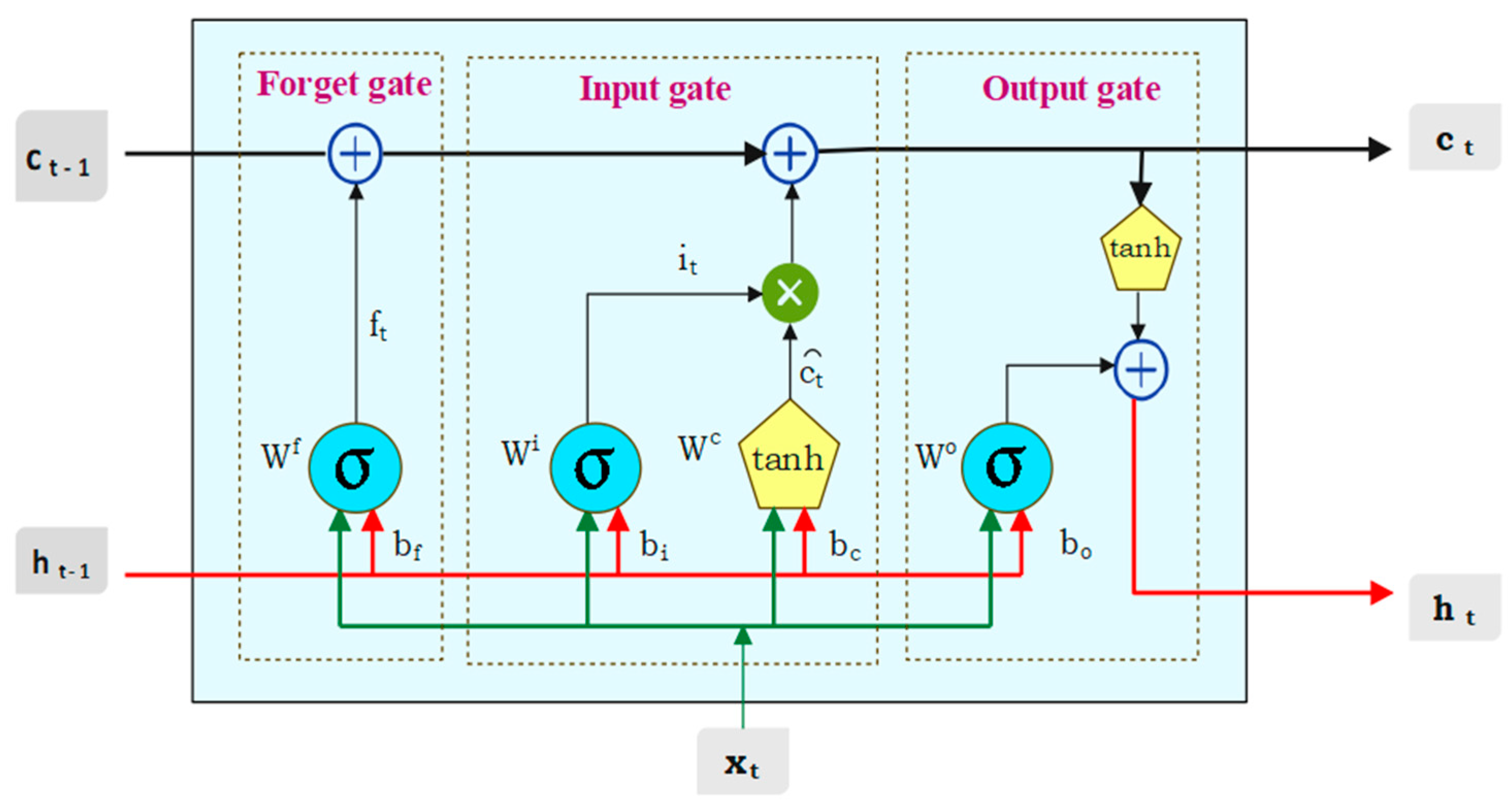
20]. Different approaches relying on RNN have been implemented to forecast the prices of agricultural products. Then, long short-term memory (LSTM) [21] was first introduced by Hochreiter and Schmidhuber in 1997, as an extension of RNN that solves the problem of exploding and vanishing gradients more effectively than the conventional RNN models. Chen et al. [22] developed a web-based automated system for predicting agriculture commodity prices. Their study revealed that the LSTM model demonstrated lower error rates compared to other machine learning models, particularly when handling extensive historical data from Malaysia. Gu et al. [23] proposed dual input attention long short-term memory (DIA-LSTM) for the efficient prediction of agricultural commodity prices like cabbage and radish in the South Korean market.
Cakici et al. [24] found that equity anomalies can predict aggregate market returns, as their predictability, if any, is confined to specific anomalies and methodological choices. Dong et al. [25] applied an array of shrinkage methods, incorporating machine learning, forecast combination, and dimension reduction, to effectively capture predictive signals in a high-dimensional environment. Incorporating wavelets as a preprocessing tool has provided a new perspective on the analysis of data characterized by noise [26]. The denoising process, one of the earliest applications of the discrete wavelet transform (DWT), is designed to eliminate small segments of the signal identified as noise [27]. Wavelet-based approaches are commonly used as versatile tools for both the analysis and synthesis of multicomponent signals, particularly for tasks such as noise removal. Removing noise from the signal not only expedites the processing of analysis but also enhances the efficiency of the model [28]. Paul et al. [29] conducted a comparative analysis of various wavelet functions, including Haar, Daubechies (D4), D6, and LA8, to assess their performance in forecasting the prices of tomatoes. Shabri et al. [30] suggested that the augmentation of the wavelet technique in the SVM model results in improved forecasting performance compared to classical SVM and demonstrated its superiority over ANN. Garai et al. [31] presented a methodology that combines stochastic and machine learning models, alongside the utilization of wavelet analysis, for the prediction of agricultural prices.
Chen et al. [32] used the wavelet analysis as a denoising tool along with LSTM for the prediction the prices of Agricultural products in China. Liang et al. [33] put forth a novel threshold-denoising function with the aim of decreasing the distortion levels in signal reconstruction. The outcomes unequivocally demonstrated that the proposed function, when combined with the LSTM model, surpassed the performance of other conventional models. Zhou et al. [34] evaluated the deep neural network (DNN) models for equity-premium forecasting and compared them with ordinary least squares (OLS) and historical average (HA) models. They found that augmenting DNN models with 14 additional variables enhanced their forecasting performance, showcasing their adaptability and superiority in equity-premium prediction. Jaseena and Kovoor [35] utilized wavelet transform to decompose wind speed data into high and low frequency subseries. Subsequently, they forecasted the low and high frequency subseries using LSTM and SVR, respectively. Peng et al. [36] made an attempt to predict the stock movement for the next 11 days (medium-term) by using multiresolution wavelet reconstruction and RNN. Singla et al. [37] proposed an ensemble model to forecast the 24-h ahead solar GHI for the location of Ahmadabad, Gujarat, India, by combining wavelet and BiLSTM networks (WT-BiLSTM (CF)). They also compared the forecasting performance of WT-BiLSTM (CF) with unidirectional LSTM, unidirectional GRU, BiLSTM, and wavelet-based BiLSTM models. Yeasin and Paul [38] proposed an ensemble model consisting of 13 forecasting models including five deep learning, five machine learning, and three stochastic models for forecasting vegetable prices in India. Liang et al. [39] constructed an Internet-based consumer price index (ICPI) from Baidu and Google searches using principal component analysis. Transfer entropy quantifies information flow between online behavior and future markets. The GWO-CNN-LSTM model, incorporating ICPI and transfer entropy, forecasts daily prices of corn, soybean, PVC, egg, and rebar futures. Cai et al. [40] had proposed a variational mode decomposition method along with deep learning model to forecast the hourly PM2.5 concentration. Deng et al. [41] used multivariate empirical mode decomposition along with LSTM while dealing with forecasting of multi-step-ahead stock prices. Lin et al. [42] decomposed the crude oil price data using wavelet transform and fed into a BiLSTM-Attention-CNN model for predicting the future price.
However, there exists a very low number of studies related to the gain in prediction accuracy of the models based on wavelet decomposed series compared to usual benchmark models. The present study illustrates this in detail, with application of machine learning, deep learning, and stochastic models in conjunction with wavelet denoising.

3. Methodology

3.1. ARIMA

ARIMA is often considered the foundational cornerstone in the realm of predictive modeling, which was given by Box and Jerkins in 1970 [43]. The ARIMA modeling process revolves around four key steps. These are the identification of the model, estimation of the parameters, diagnostic checking, and forecasting. This model class relies on the fundamental assumption that time series should exhibit stationarity and the future values of a time series result from a linear combination of previous observations and white noise components. Then, ARMA (p, q) can be written as:
y t = α 1 y t 1 + α 2 y t 2 + + α p y t p θ 1 ε t 1 θ 2 ε t 2 θ q ε t q + ε t
or equivalently (using backshift operator B ) by:
α B y t = θ B ε t
where:
α B = 1 α 1 B α 2 B 2 α p B p
θ B = 1 θ 1 B θ 2 B 2 θ p B p
ARMA models require stationary data, but real-world data in various fields is often non-stationary. By applying differencing, data can be made stationary, leading to the development of ARIMA models [39], represented as ARIMA (p, d, q). Then, the model is written as:
α B 1 B d y t = θ B ε t  
where ε t is identically and independently distributed (IID) as N 0 , σ 2 . The parameters ranging from α 1 to α p represent the autoregressive (AR) coefficients, while θ1 to θq denote the moving average (MA) coefficients.

3.2. Artificial Neural Networks

ANN models are built on the concept of neurons that interact by transmitting signals through weighted connections to one another [44]. These networks emulate the way biological neurons exchange information in the brain [45]. In ANN models, each neuron is connected to all preceding neurons and passes the layers through links. In the input layer, each input value is treated as a neuron. To enable the success of an ANN, all input values are initially weighted, and the weighted values are then processed within the hidden layers, where each neuron generates output values. This process allows ANNs to learn and make predictions or classifications based on the weighted inputs and the network’s architecture. The output value of the neuron can be represented by the formula:
O = θ   j = 1 n w j x j + w 0  
where O and x j represent the output and input values to the neuron, respectively, w 0 is the bias term, w j ’s is the weightage related to each input, and θ represents the activation function. Figure 1 explained the basic architecture of ANN model. The flexibility of an artificial neural network (ANN) lies in its adaptable architecture, allowing easy adjustments to the number of layers and neurons in each layer. Unlike certain modeling approaches, ANN does not demand prior assumptions like data stationarity during the model-building process. As a result, the network’s structure is primarily guided by the unique characteristics of the data being analyzed.

3.3. Support Vector Regression (SVR)

SVR is centered on the principles of statistical learning theory and the rule of structural risk minimization [41]. It has proven to be highly effective for modeling and predicting non-linear systems by minimizing the upper limit of generalization error [16]. The SVR model can be expressed mathematically as follows:
  f x = ( z . x ) + b     w i t h     w R N , b R
where z stands for the weight vector, while x denotes the high-dimensional feature space resulting from a non-linear transformation of the input space and b is the bias. The estimation of the weight vector z and bias b involves the minimization of the regularized risk function:
R ( C ) = 1 2 | z | 2 + C 1 p   i = 1 t L ε f x i , y i
Within the regularized risk function, the initial term 1 2 | z | 2 serves as the regularization component, regulating the model’s capacity. The second term, 1 p i = 1 t L ε f x i , y i , represents the empirical error. The constant ‘C’ plays a crucial role as the regularization parameter, influencing the balance between empirical risk and regularization within the model. In the case of the SVR model, ε -insensitivity loss function is used and can be expressed as:
L ε f x i , y i = f x i y i ε , f x i y i ε 0 ,   otherwise    
where ε denotes the tube size. Minimizing Equation (7) can be expressed as solving the following the primal optimization problem:
ξ i and ξ i * are positive slack variables that quantify the gap between actual values and the respective boundary values within the ε tube. Equation (7) can also be written as:
f x , z = f x , α , α * = i α i α i * x , x i + b  
The kernel function ∅(.) is employed to transform the non-linear dataset into a higher-dimensional feature space, where it is assumed to be linear. For a function to be considered a kernel function, it must satisfy Mercer’s condition, as outlined by Mercer in 1909. The data calibration of SVR model are presented in the Figure 2.

3.4. Long Short Term Memory

The LSTM incorporates a cell state that traverses the network, allowing information to be added or removed through gating mechanisms. Thus, the LSTM model is structured around three vital gate mechanisms: the forget gate, input gate, and output gate [24]. These gate structures serve as the fundamental building blocks of the LSTM, empowering it to effectively process and forecast important information, even when dealing with long-term time intervals and temporal delays in time series data [46]. The architecture of the single LSTM cell is presented in Figure 3.
Forget Gate: It involves a sigmoid layer that decides which information needs to be discarded from the cell state. It accomplishes this by merging the current input x t with the output of the preceding LSTM unit, h t 1 .
f t = σ W f x t + U f h t 1 + b f
Input Gate: It consists of two components. The first layer is a sigmoid layer, responsible for making decision regarding value updates. The following layer is a tanh layer, generating a vector of new candidate values, denoted as C ~ t , which can be integrated into the cell state.
i t = σ W i x t + U i h t 1 + b i
C ~ t = t a n h W c x t + U c h t 1 + b c
Then, we need to update the old cell state C t 1 into new state C t . Update includes forgetting the old information by multiply the f t with C t 1 and adding the new information by multiplying i t with C ~ t .
C t = f t × C t 1 + i t × C ~ t
Output gate: The output gate is instrumental in defining the value of the next hidden state h t , which captures information from prior inputs. It initiates by taking both the current state and the previous hidden state values into a sigmoid function. Subsequently, the new cell state C t , which is derived from the existing cell state, undergoes additional processing through the tanh function.
O t = σ W o x t + U o h t 1 + b o
h t = O t × tanh ( C t )
where W * and U * represent the weight of current input x t and output of previous LSTM unit h t 1 , respectively, while b * is bias vector and * represents the corresponding gates.

3.5. Wavelet-Based Denoising

The main concept behind using wavelet transforms and their inverses is that it allows for a multi-resolution analysis of a signal. Different wavelet coefficients represent different frequency components of the signal at various resolutions or scales. This is particularly useful in applications like signal processing, image compression, and denoising. The denoising process can be defined as the removal of noise while preserving and without distorting the quality of the processed signal or image. Wavelet transform helps in denoising by decomposing the signal into different levels. The general procedure of noise removal takes place by three main steps. The initial step involves decomposition, wherein the noisy data undergoes transformation into an orthogonal domain. The second step entails various processing operations on the obtained coefficients. The final step involves the data being transformed back into its original domain through a reconstruction process. The time series data are decomposed by passing through the high pass and low pass filter. The high pass filter produces the high-frequency detail components, while the low-pass filter generates the low-frequency approximate components of the signal. Both components of the filter have an equal bandwidth. Subsequently, the next step involves iterating the aforementioned process for the low-frequency component to acquire the two decomposed components.
Step 1: The time series x(t) under wavelet transform is expressed as:
x t = j a i , j ω i , j t + j d i , j ψ i , j t + j d i 1 , j ψ i , j t + + j d 1 , j ψ i , j t
s i t = k s i , j ω i , j t
D i t = k d i , j ψ i , j t
The original signal can be represented as the sum of detailed and approximate components as follows:
x t = J = 1 i D i t + S i t
where J denotes the level of decomposition, ranging from 1 to i; j is the translation parameter; ψ i , j ( t ) and ω i , j ( t ) represent the parent wavelet pairs; s i , j denotes the scaling coefficient of father wavelet ω i , j ( t ) and d i , j is the detail coefficient of mother wavelet ψ i , j ( t ) ; D i ( t ) represent the high-frequency component signal; and S i ( t ) is the low-frequency component signal.
Step 2: Each decomposed component separately is fed into the benchmark models. Optimal hyperparameters for the model are chosen by examining its performance on a distinct validation set. After fine- tuning, the model undergoes the evaluation on test data by subjecting each series to the LSTM model, leading to the accurate prediction of price series.
Step 3: The inverse wavelet transform (IWT) is the mathematical operation that reconstructs a signal from its wavelet coefficients. The prediction obtained from each series coefficient is subjected to IWT for wavelet reconstruction. The outlook of analysis performed is presented in Figure 4.

4. Result and Discussion

4.1. Data Description

The current study focused on the monthly wholesale price data of three important spices (i.e., turmeric, coriander, and cumin) from different markets of India, where data series were collected from the AGMARKNET Portal http://agmarknet.gov.in/ (accessed on 3 July 2023) for the period of January 2010 to December 2022. Turmeric data were gathered from 18 distinct markets, while coriander and cumin data were obtained from 27 markets each. The choice of markets and commodities was determined by their significant market share and their representative characteristics within their respective categories. The overall price for each commodity was calculated as the weighted average price across all markets for that specific commodity. The weight assigned to each market was determined by the inverse of the arrival quantity:
a g g r e g a t e d   p r i c e t = i = 1 N q u a n t i t y i , t × p r i c e i , t i = 1 N q u a n t i t y i , t
where N is the number of markets in that commodity and t is time period. The price patterns of three spices are illustrated in Figure 4. The dataset consists of a total of 156 observations across all commodities. The final 29 observations were set aside for testing and post-sample prediction, leaving 127 observations for model development in each case. Table 1 represents the descriptive statistics of different commodities. 
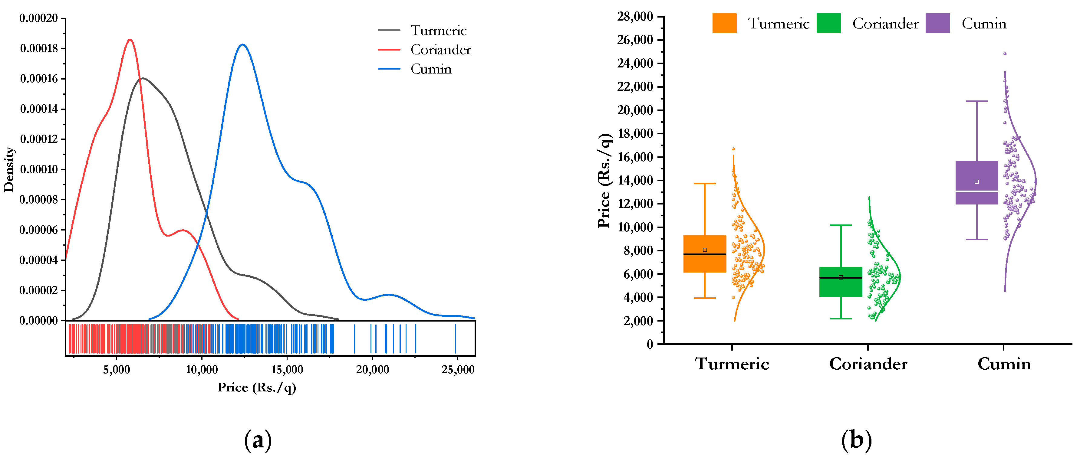
Table 1 indicates that all the prices series were non-normal and have high kurtosis. The Jarque–Bera test and Shapiro–Wilk’s test are statistical methods employed to evaluate whether a dataset follows normal distribution. The null hypothesis of both the tests are that data follow a normal distribution. It is inferred from the table that all the three commodities are non-normal. The variability in price is less for cumin as compared to other two spices. The kernel density and the box-plot of different price series are plotted in Figure 5. Figure 5 also demonstrates high kurtosis and positive skew.

4.2. Application of Benchmark Models

The primary contenders in the field of predictive modelling start with ARIMA. The process initiates with checking the stationarity of the underlying data through an augmented Dickey–Fuller (ADF) test and the results are outlined in Table 2. All the three series exhibited non-stationarity which is converted into stationarity by differencing. The order of the model was tentatively identified using the autocorrelation function (ACF) and partial autocorrelation function (PACF). Ultimately, the selection of the best model for individual commodity prices was performed based on the minimum values of Akaike Information Criterion (AIC) and Bayesian Information Criterion (BIC).
Before proceeding for the application of machine learning and deep learning techniques, the presence of volatility clustering was tested by means of the autoregressive conditional heteroscedastic-Lagrange multiplier (ARCH-LM) test. It is found that for all three series, the test is not significant indicating absence of any volatility clustering.
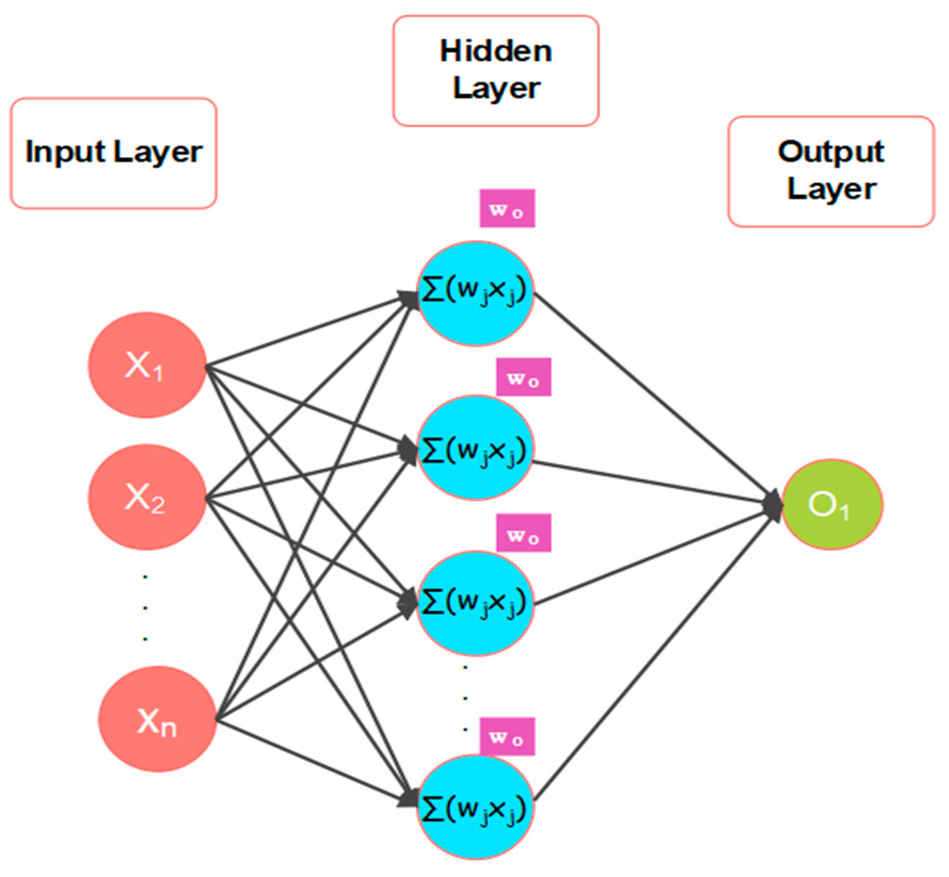
The individual price series was subjected to ANN, SVR and LSTM model. In the process of developing an ANN, selection of input lag value is a crucial step. Here, the input lag value was selected as 12 with the help of ACF. The ANN model used in this study is the standard two-layer feed forward network. The efficiency of the model can be improved by finding the best set of hyperparameter values for the training dataset. The hyperparametric search space for ANN were the number of nodes per layer = {6, 7, 8, 9,10, 11, 12}, number of epochs = {10 to 100 with step 10}, and batch size = {16, 32, 64, 128}. The hyperparameters were optimized by using grid search method.
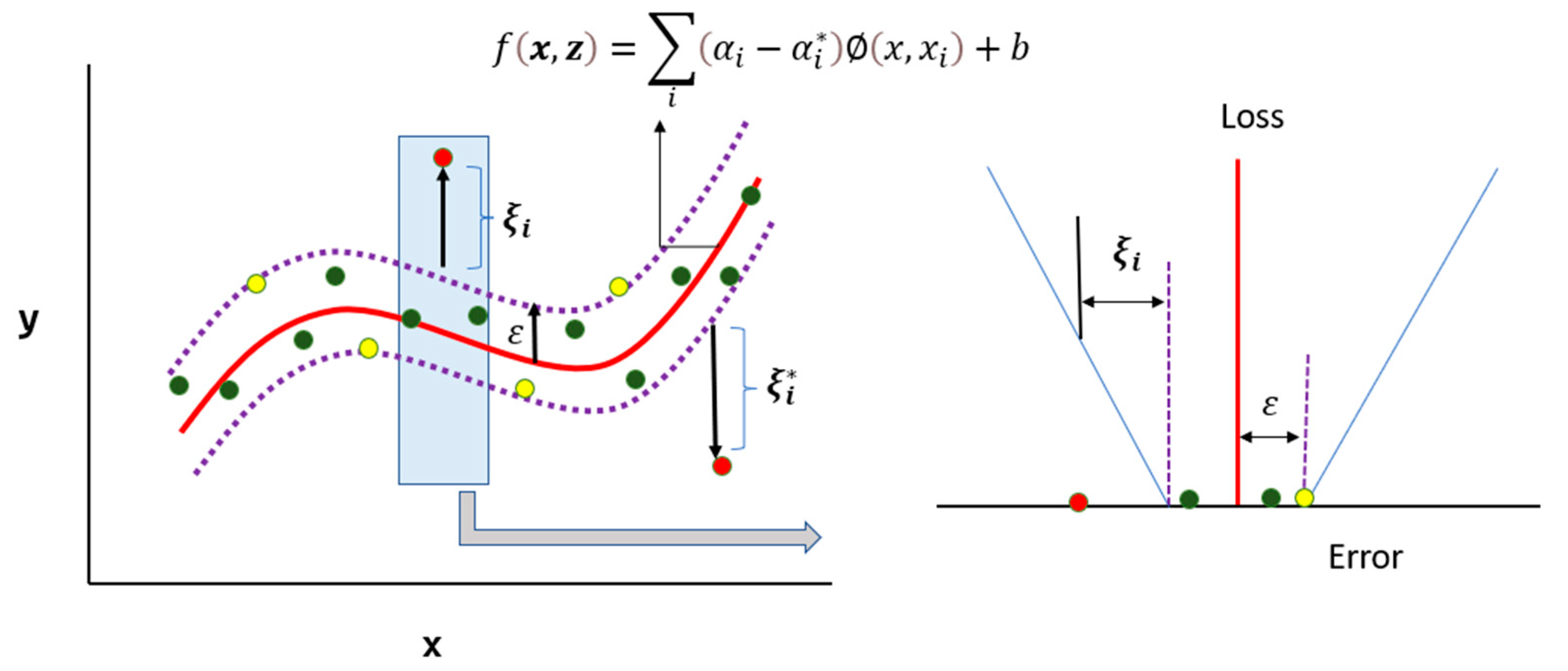
For building the SVR model, the actual value yt was assumed to be a function of its previous lag values. The model uses an RBF kernel, and the hyperparameters C (Regularization parameter), ε (epsilon), and γ (kernel width) were optimized using grid search over the following ranges: C = {1, 10,…, 1000 with step 10.}, ε = { 0.01, 0.02,…, 0.30}, γ = {3, 4,…, 15}. In order to build LSTM model, lag values were established at 12. The Hyperparameter search space for LSTM were the number of LSTM units = {32, 64, 128}, number of epochs = {50, 100, 200}, and batch size = {16, 32, 64, 128}.
The best hyperparameters are selected based on the performance of the model on a hold-out validation set. Once the hyperparameters have been tuned, the model is evaluated on a test set to assess its performance on unseen data. The model’s performance on the test data can be evaluated using a variety of metrics, such as the mean absolute error (MAE), root mean square error (RMSE), and mean absolute percentage error (MAPE).
Table 3 provides a clear overview of various accuracy measures of different models, including LSTM, SVR, ANN, and ARIMA, across the crops turmeric, coriander, and cumin. For turmeric, LSTM demonstrated a substantial 21.4% reduction in RMSE compared to SVR. In the case of coriander, LSTM achieved an impressive 40.7% reduction in RMSE relative to SVR. For cumin, LSTM showcased a significant 37.3% decrease in RMSE compared to SVR. For all the three crops (turmeric, coriander, cumin), the LSTM model consistently outperformed other models in terms of RMSE, MAPE, and MAE, suggesting they are generally better at capturing the underlying patterns in the data.

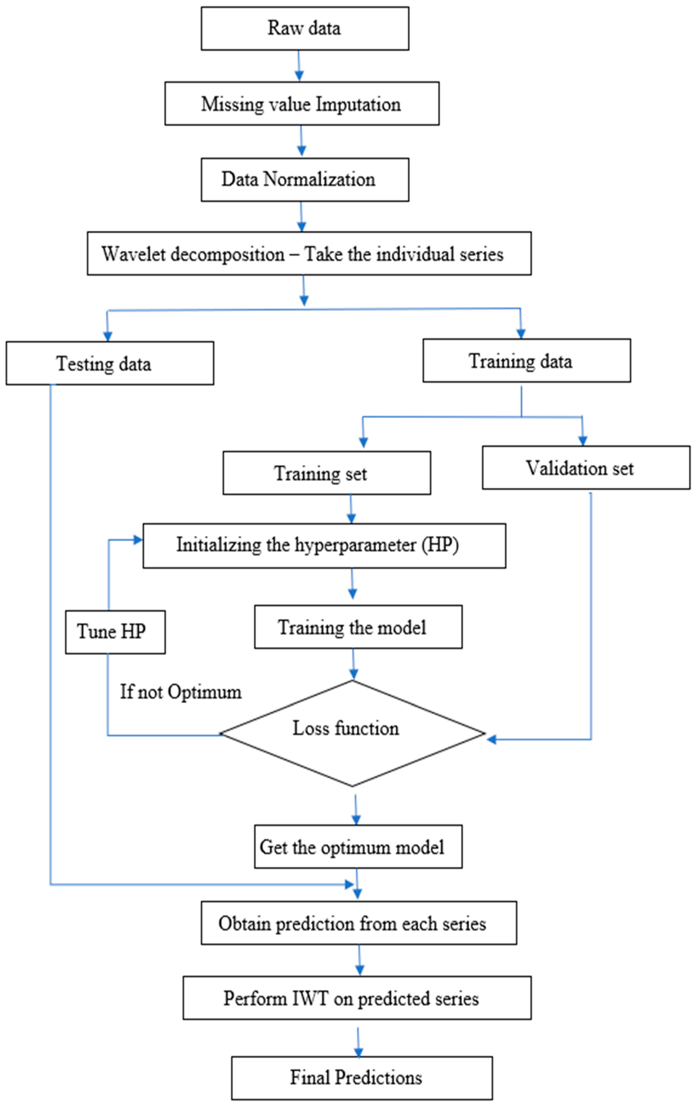
4.3. Denoising Using Wavelet

While there are numerous methods available for predicting prices series, they do not consistently meet expected performance levels, as each method comes with its own set of advantages and disadvantages. Denoising helps us to filter out this extraneous noise, enabling the model to focus on the relevant patterns and relationships in the data. So, the original series were denoised using wavelet transform before applying the model. The Haar wavelet filter was used for wavelet transformation. The maximum ( J 1 = l o g 2 N ) and minimum ( J 0 = log N ) levels of decomposition for price series were 7 and 5, respectively. So, each series was decomposed at all three levels and fed as input to ARIMA, ANN, SVR, and LSTM models. The hyperparameters of the models were tuned using a grid search over a range of possible values as mentioned before. Table 4, Table 5 and Table 6 represent the accuracy measure of various models on the test data with different levels of decomposition (bold denotes the lowest of each accuracy metrics). Here, H5, H6, and H7 represent the wavelet decomposition with the Haar filter and level of decomposition as 5, 6, and 7, respectively.
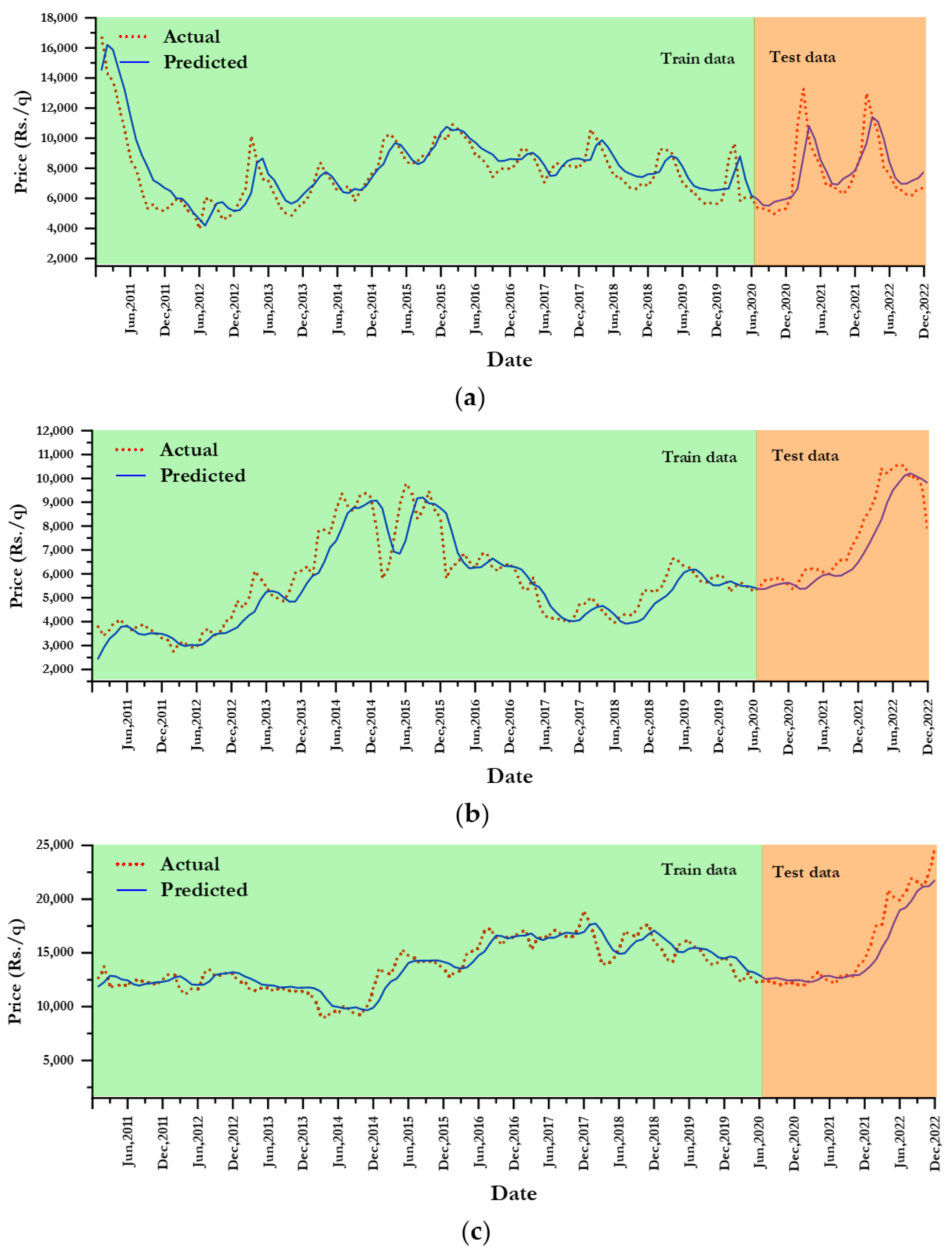
For turmeric, decomposition level H6 was optimal for WLSTM, offering the highest accuracy across all metrics, whereas WSVR and WARIMA performed best at H7 and H5 decomposition levels, respectively. For coriander, decomposition level H6 exhibited the lowest RMSE, MAPE, and MAE, indicating better predictive accuracy compared to other levels across all models (WLSTM, WSVR, and WANN), except WARIMA. For cumin prices, the most effective decomposition level was H7 and H5 for WLSTM and WARIMA, respectively, presenting the lowest RMSE, MAPE, and MAE. Across all models in cumin, decomposition level H6 tended to consistently offer the best predictive accuracy, as it frequently displayed the lowest values for RMSE, MAPE, and MAE. The WLSTM model outperformed the other models (WSVR, WANN, and WARIMA) on all three datasets (turmeric, coriander, and cumin). The performance of the best fitted model, i.e., WLSTM, for both training and testing sets is presented in Figure 6.

4.4. Impact of Denoising

Table 7 explains the influence of denoising in the current dataset. Among the different levels of decomposition, the optimum level of decomposition was selected based on the minimum values of accuracy measures and subsequently compared with a benchmark model. The percentage decrease (%↓) in error was calculated for finding the improvement achieved by the wavelet-based denoising model (WLSTM, WSVR, WANN, WARIMA) over their respective baseline models. In all three commodities, percentage of error reduction due to denoising was greater than 30% when compared to traditional LSTM. For turmeric, WLSTM achieved a significant 35.22% reduction in RMSE compared to LSTM. Coriander showed an even more substantial reduction of 42.38% in RMSE with WLSTM. Cumin also exhibited 34.75% reduction in RMSE when using WLSTM. WSVR demonstrated superior performance compared to SVR, achieving substantial reductions in RMSE of 30.46%, 21.67%, and 28.68% for turmeric, coriander, and cumin, respectively. Similarly, wavelet-based ANN and ARIMA also had a significant reduction in error when compared to benchmark models.
The technique for order preference by similarity to ideal solution (TOPSIS) has been applied for finding the best model with respect to each of the series under consideration. Equal weightage has been given to each of the performance measures, i.e., RMSE, MAPE, and MAE. The TOPSIS scores and ranks were computed for wavelet-based denoising models and the same is presented in Table 8. Table 8 indicates that the WLSTM occupied the top three ranks in all the price series. Moreover, the Diebold–Mariano (DM) test was applied to see the significant differences in predictive accuracy between the two models. The result of the DM test is reported in Table 9, which indicates the significant differences between the wavelet-based denoising model and the individual benchmark model. Overall, the results clearly demonstrated the effectiveness of wavelet-based denoising in reducing errors across the different spice crops and forecasting techniques.

5. Conclusions

In the current study, the effect of wavelet-based denoising was illustrated on the monthly wholesale prices of three pivotal spices—turmeric, coriander, and cumin, collected from the diverse markets across India. Wavelet denoising involves the application of methods or algorithms to filter out the extraneous noise, enabling the model to focus on the relevant patterns and relationships in the data. The various levels of decomposition were taken into account for studying the effectiveness of denoising. The benchmark modeling phase commenced with the deployment of the ARIMA model, a widely recognized time series forecasting method. The modeling spectrum expanded to include artificial neural networks (ANN), support vector regression (SVR), and long short-term memory (LSTM) models. These models were subjected to hyperparameter optimization through a grid search method, aiming to fine-tune the parameters for optimal performance. Also, the efficacy of wavelet-based denoising was assessed by comparing it with a benchmark model using three accuracy metrics, namely, RMSE, MAPE, and MAE. The results on the test set unequivocally indicated the consistent superiority of LSTM across all three spices, showcasing its adeptness in capturing the intricate patterns inherent in the data. The performance of each model may vary with different decomposition levels, emphasizing the importance of carefully selecting the appropriate level based on specific modeling objectives and metric priorities. The comparative analysis between the wavelet-based denoising models (WLSTM, WSVR, WANN, WARIMA) and their traditional counterparts provided resounding affirmation regarding the substantial enhancement in predictive accuracy introduced by wavelet transforms. Across all three spices, denoising consistently led to significant reductions in error metrics, with percentage decreases ranging from 30% to over 40%.
In general, Wavelet LSTM at H6 appears to be a robust choice for accurate price predictions across all spices. The order of preference for model performance, based on the provided metrics, could be WLSTM > WARIMA > WSVR > WANN for turmeric, WLSTM > WANN > WSVR > WARIMA for coriander, and WLSTM > WSVR > WANN> WARIMA for cumin. The final step in the comparative analysis involved the application of the TOPSIS method. This method offered a comprehensive evaluation, considering all three performance metrics with equal weightage. The TOPSIS scores and ranks reaffirmed WLSTM’s superiority, consistently placing it at the forefront across all decomposition levels and spices. The DM test also resulted in significant differences in prediction accuracy between wavelet-based models with that of the usual model. Indeed, the computational intensity of wavelet-based denoising, particularly with sophisticated algorithms, is a notable limitation. Processing large datasets or implementing real-time denoising may pose challenges in terms of computational resources. The effectiveness of wavelet-based denoising is highly dependent on the choice of the wavelet function. The other wavelet filters may be explored in future research to gain a clear idea about the selection of suitable filter and level for a specific pattern existed in the time series.

Author Contributions

Conceptualization, R.K.P. and C.T.; methodology, C.T., R.K.P. and M.Y.; software, C.T. and M.Y.; validation, C.T., M.Y. and A.K.P.; formal analysis, C.T.; investigation, C.T. and R.K.P.; resources, R.K.P.; data curation, C.T.; writing—original draft preparation, C.T.; writing—review and editing, C.T., M.Y. and R.K.P.; visualization, C.T. and A.K.P.; supervision, R.K.P. All authors have read and agreed to the published version of the manuscript.

Funding

This research received no external funding.

Data Availability Statement

Data will be available on reasonable request.

Acknowledgments

The authors are thankful to The Graduate School, ICAR-Indian Agricultural Research Institute, New Delhi, and Director, ICAR-Indian Agricultural Statistics Research Institute, New Delhi, for providing the required facility.

Conflicts of Interest

The authors declare no conflicts of interest.

References

  1. Oktoviany, P.; Knobloch, R.; Korn, R. A machine learning-based price state prediction model for agricultural commodities using external factors. Decis. Econ. Financ. 2021, 44, 1063–1085. [Google Scholar] [CrossRef]
  2. Cerqueira, V.; Torgo, L.; Soares, C. A case study comparing machine learning with statistical methods for time series forecasting: Size matters. J. Intell. Inf. Syst. 2022, 59, 415–433. [Google Scholar] [CrossRef]
  3. Khan, F.; Urooj, A.; Khan, S.A.; Alsubie, A.; Almaspoor, Z.; Muhammadullah, S. Comparing the Forecast Performance of Advanced Statistical and Machine Learning Techniques Using Huge Big Data: Evidence from Monte Carlo Experiments. Complexity 2021, 2021, 6117513. [Google Scholar] [CrossRef]
  4. Rioul, O.; Vetterli, M. Wavelets and Signal Processing. IEEE Signal Process Mag. 1991, 8, 14–38. [Google Scholar] [CrossRef]
  5. Gidwani, B.; Bhattacharya, R.; Shukla, S.S.; Pandey, R.K. Indian spices: Past, present and future challenges as the engine for bio-enhancement of drugs: Impact of COVID-19. J. Sci. Food Agric. 2022, 102, 3065–3077. [Google Scholar] [CrossRef] [PubMed]
  6. Sharangi, A.B.; Pandit, M.K. Indian Spices: The Legacy, Production and Processing of India’s Treasured Export; Springer: Berlin/Heidelberg, Germany, 2018; pp. 341–357. [Google Scholar]
  7. Valasan, A. Spices Export from Kerala Current Trends & Opportunities Ahead. IRA-Int. J. Manag. Soc. Sci. 2016, 5, 54–65. [Google Scholar]
  8. Srinu, N.; Bindu, B.H. A Review on Machine Learning and Deep Learning based Rainfall Prediction Methods. In Proceedings of the 3rd International Conference on Power, Energy, Control and Transmission Systems, Chennai, India, 8–9 December 2022. [Google Scholar]
  9. Ashok, S.P.; Pekkat, S. A systematic quantitative review on the performance of some of the recent short-term rainfall forecasting techniques. J. Water Clim. Change 2022, 13, 3004. [Google Scholar] [CrossRef]
  10. Kaur, J.; Parmar, K.S.; Singh, S. Autoregressive models in environmental forecasting time series: A theoretical and application review. Environ. Sci. Pollut. Res. 2023, 30, 19617–19641. [Google Scholar] [CrossRef]
  11. Mao, L.; Huang, Y.; Zhang, X.; Li, S.; Huang, X. ARIMA model forecasting analysis of the prices of multiple vegetables under the impact of the COVID-19. PLoS ONE 2022, 17, e0271594. [Google Scholar] [CrossRef]
  12. Liakos, K.G.; Busato, P.; Moshou, D.; Pearson, S.; Bochtis, D. Machine Learning in Agriculture: A Review. Sensors 2018, 18, 2674. [Google Scholar] [CrossRef]
  13. Mahto, A.K.; Alam, M.A.; Biswas, R.; Ahmad, J.; Alam, S.I. Short-Term Forecasting of Agriculture Commodities in Context of Indian Market for Sustainable Agriculture by Using the Artificial Neural Network. J. Food Qual. 2021, 2021, 1–13. [Google Scholar] [CrossRef]
  14. Astudillo, G.; Carrasco, R.; Fernández-Campusano, C.; Chacón, M. Copper price prediction using support vector regression technique. Appl. Sci. 2020, 10, 6648. [Google Scholar] [CrossRef]
  15. Jeong, M.; Lee, Y.J.; Choe, Y. Forecasting Agricultural Commodity Price: The Case of onion. Quest J. J. Res. Humanit. Soc. Sci. 2017, 5, 78–81. [Google Scholar]
  16. Zhang, D.; Chen, S.; Liwen, L.; Xia, Q. Forecasting Agricultural Commodity Prices Using Model Selection Framework with Time Series Features and Forecast Horizons. IEEE Access 2020, 8, 28197–28209. [Google Scholar] [CrossRef]
  17. Paul, R.K.; Yeasin, M.; Kumar, P.; Kumar, P.; Balasubramanian, M.; Roy, H.S.; Paul, A.K.; Gupta, A. Machine learning techniques for forecasting agricultural prices: A case of brinjal in Odisha, India. PLoS ONE 2022, 17, e0270553. [Google Scholar] [CrossRef]
  18. Paul, R.K.; Yeasin, M.; Kumar, P.; Paul, A.K.; Roy, H.S. Deep Learning Technique for Forecasting Price of Cauliflower. Curr. Sci. 2023, 124, 1065–1073. [Google Scholar]
  19. Liu, M.; Qin, H.; Cao, R.; Deng, S. Short-Term Load Forecasting Based on Improved TCN and DenseNet. IEEE Access 2022, 10, 115945–115957. [Google Scholar] [CrossRef]
  20. Kapoor, A.; Pathiraja, S.; Marshall, L.; Chandra, R. DeepGR4J: A deep learning hybridization approach for conceptual rainfall-runoff modelling. Environ. Model. Softw. 2023, 169, 105831. [Google Scholar] [CrossRef]
  21. Hochreiter, S.; Schmidhuber, J. Long Short-Term Memory. Neural Comput. 1997, 9, 1735–1780. [Google Scholar] [CrossRef]
  22. Chen, X.; He, G.; Chen, Y.; Zhang, S.; Chen, J.; Qian, J.; Yu, H. Notice of Retraction: Short-term and local rainfall probability prediction based on a dislocation support vector machine model using satellite and in-situ observational data. IEEE Access 2021, 1. [Google Scholar] [CrossRef]
  23. Gu, Y.H.; Jin, D.; Yin, H.; Zheng, R.; Piao, X.; Yoo, S.J. Forecasting Agricultural Commodity Prices Using Dual Input Attention LSTM. Agriculture 2022, 12, 256. [Google Scholar] [CrossRef]
  24. Cakici, N.; Fieberg, C.; Metko, D.; Zaremba, A. Do anomalies really predict market returns? New data and new evidence. Rev. Financ. 2023, rfad025. [Google Scholar] [CrossRef]
  25. Dong, X.; Li, Y.; Rapach, D.E.; Zhou, G. Anomalies and the expected market return. J. Financ. 2022, 77, 639–681. [Google Scholar] [CrossRef]
  26. Paul, R.K.; Garai, S. Wavelets Based Artificial Neural Network Technique for Forecasting Agricultural Prices. J. Indian Soc. Probab. Stat. 2022, 23, 47–61. [Google Scholar] [CrossRef]
  27. Lang, M.; Guo, H.; Odegard, J.E.; Burrus, C.S.; Wells, R.O. Noise reduction using an undecimated discrete wavelet transform. Signal Process. Lett. IEEE 1996, 3, 10–12. [Google Scholar] [CrossRef]
  28. Boto-Giralda, D.; Díaz-Pernas, F.J.; González-Ortega, D.; Díez-Higuera, J.F.; Antón-Rodríguez, M.; Martínez-Zarzuela, M.; Torre-Díez, I. Wavelet-Based Denoising for Traffic Volume Time Series Forecasting with Self-Organizing Neural Networks. Comput. Aided Civ. Infrastruct. Eng. 2010, 25, 530–545. [Google Scholar] [CrossRef]
  29. Paul, R.K.; Garai, S. Performance comparison of wavelets-based machine learning technique for forecasting agricultural commodity prices. Soft Comput. 2021, 25, 12857–12873. [Google Scholar] [CrossRef]
  30. Shabri, A.; Hamid, M.F.A. Wavelet-support vector machine for forecasting palm oil price. Malays. J. Fundam. Appl. Sci. 2019, 15, 398–406. [Google Scholar] [CrossRef]
  31. Garai, S.; Paul, R.K.; Rakshit, D.; Yeasin, M.; Emam, W.; Tashkandy, Y.; Chesneau, C. Wavelets in Combination with Stochastic and Machine Learning Models to Predict Agricultural Prices. Mathematics 2023, 11, 2896. [Google Scholar] [CrossRef]
  32. Chen, Q.; Lin, X.; Zhong, Y.; Xie, Z. Price prediction of agricultural products based on wavelet analysis-LSTM. In Proceedings of the 2019 IEEE International Conference on Parallel and Distributed Processing with Applications, Big Data and Cloud Computing, Sustainable Computing and Communications, Social Computing and Networking, ISPA/BDCloud/SustainCom/SocialCom (IEEE), Xiamen, China, 16–18 December 2019; pp. 984–990. [Google Scholar]
  33. Liang, X.; Ge, Z.; Sun, L.; He, M.; Chen, H. LSTM with wavelet transform based data preprocessing for stock price prediction. Math. Probl. Eng. 2019, 2019, 1340174. [Google Scholar] [CrossRef]
  34. Zhou, X.; Zhou, H.; Long, H. Forecasting the equity premium: Do deep neural network models work? Mod. Financ. 2023, 1, 1–11. [Google Scholar] [CrossRef]
  35. Jaseena, K.U.; Kovoor, B.C. Decomposition-based hybrid wind speed forecasting model using deep bidirectional LSTM networks. Energy Convers. Manag. 2021, 234, 113956. [Google Scholar] [CrossRef]
  36. Peng, L.; Chen, K.; Li, N. Predicting Stock Movements: Using Multiresolution Wavelet Reconstruction and Deep Learning in Neural Networks. Information 2021, 12, 388. [Google Scholar] [CrossRef]
  37. Singla, P.; Duhan, M.; Saroha, S. An ensemble method to forecast 24-h ahead solar irradiance using wavelet decomposition and BiLSTM deep learning network. Earth Sci. Inform. 2022, 15, 291–306. [Google Scholar] [CrossRef]
  38. Yeasin, M.; Paul, R.K. OptiSembleForecasting: Optimization based ensemble forecasting using MCS algorithm and PCA based error index. J. Supercomput. 2023, 80, 1568–1597. [Google Scholar] [CrossRef]
  39. Liang, J.; Jia, G. China futures price forecasting based on online search and information transfer. Data Sci. Manag. 2022, 5, 187–198. [Google Scholar] [CrossRef]
  40. Cai, P.; Zhang, C.; Chai, J. Forecasting hourly PM 2.5 concentrations based on decomposition-ensemble-reconstruction framework incorporating deep learning algorithms. Data Sci. Manag. 2023, 6, 46–54. [Google Scholar] [CrossRef]
  41. Deng, C.; Huang, Y.; Hasan, N.; Bao, Y. Multi-step-ahead stock price index forecasting using long short-term memory model with multivariate empirical mode decomposition. Inf. Sci. 2022, 607, 297–321. [Google Scholar] [CrossRef]
  42. Lin, Y.; Chen, K.; Zhang, X.; Tan, B.; Lu, Q. Forecasting crude oil futures prices using BiLSTM-Attention-CNN model with Wavelet transform. Appl. Soft Comput. 2022, 130, 109723. [Google Scholar] [CrossRef]
  43. Makridakis, S.; Wheelwright, S.C.; Hyndman, R.J. Forecasting Methods and Applications; John Wiley & Sons: Hoboken, NJ, USA, 2008. [Google Scholar]
  44. Feng, F.; Na, W.; Jin, J.; Zhang, J.; Zhang, W.; Zhang, Q.J. Artificial neural networks for microwave computer-aided design: The state of the art. IEEE Trans. Microw. Theory Tech. 2022, 70, 4597–4619. [Google Scholar] [CrossRef]
  45. Valiant, L.G. A theory of the learnable. Commun. ACM 1984, 27, 1134–1142. [Google Scholar] [CrossRef]
  46. Feng, G.; He, J.; Polson, N.G. Deep learning for predicting asset returns. arXiv 2018, arXiv:1804.09314. [Google Scholar]
Figure 1. Basic architecture of ANN (Source: own illustration).
Forecasting 06 00005 g001
Figure 2. Data calibration in the support vector regression model (Source: own illustration).
Forecasting 06 00005 g002
Figure 3. The architecture of the single LSTM cell (Source: own illustration).
Forecasting 06 00005 g003
Figure 4. Flowchart of the proposed algorithm (Source: own illustration).
Forecasting 06 00005 g004
Figure 5. (a) Kernal density and (b) box-plot of different spices.
Forecasting 06 00005 g005
Figure 6. Actual and predicted values of the best fitted model for price series of (a) turmeric, (b) coriander, and (c) cumin.
Forecasting 06 00005 g006
Table 1. The descriptive statistics of the price of spices.
Descriptive StatisticsTurmeric (Rs/qtl)Coriander (Rs/qtl)Cumin (Rs/qtl)
Mean7846.25093.2313,756.65
Median7236.834832.4912,844.92
Minimum3745.762265.098826.91
Maximum16,119.799484.0824,672.25
Standard Deviation2633.531753.482841.91
Kurtosis4.132.714.22
Skewness1.290.641.02
C.V. (%)33.5634.4320.66
Jarque-Bera test51.39 (<0.01)6.50 (<0.01)36.76 (<0.01)
Shapiro-Wilk’s test0.87 (<0.01)0.96 (<0.01)0.93 (<0.01)
Table 2. The stationarity test results of price series.
DataAugmented Dickey–Fuller TestKwiatkowski–Phillips–Schmidt–Shin Remarks
Statisticp-ValueStatisticp-Value
Turmeric (Rs/qtl)−2.870.210.470.04Non-Stationary
Coriander (Rs/qtl)−2.040.550.750.01Non-Stationary
Cumin (Rs/qtl)−1.610.731.080.01Non-Stationary
Table 3. Accuracy measures for different models for test data (bold denotes the lowest of each accuracy metrics).
CropModelRMSEMAPEMAE
TurmericLSTM1683.4500.1531157.435
SVR2141.5290.1821694.249
ANN2180.7290.2211612.335
ARIMA1910.8000.1201122.188
CorianderLSTM1283.6700.1551095.620
SVR1754.7180.1811244.712
ANN1637.1660.1611207.808
ARIMA2930.2910.2472216.242
CuminLSTM2374.4350.1021725.857
SVR3790.3480.1272476.648
ANN3963.810.2103767.492
ARIMA5283.0880.2393523.121
Table 4. Accuracy measures of different models on the decomposed test series (turmeric).
Turmeric PricesDecomposition LevelRMSEMAPEMAE
Wavelet LSTMWLSTM-H51211.1380.076683.887
WLSTM-H61090.6060.069662.225
WLSTM-H71143.3480.076695.462
Wavelet SVRWSVR-H51489.1570.1201054.334
WSVR-H61513.6340.1231074.154
WSVR-H71458.9600.1591234.963
Wavelet ANNWANN-H51939.7060.2121612.938
WANN-H61603.8030.1711364.857
WANN-H71522.3340.1791314.672
Wavelet ARIMAWARIMA-H51221.8040.092802.592
WARIMA-H61257.0480.097839.862
WARIMA-H71223.0240.098835.978
Table 5. Accuracy measures of different models on the decomposed test series (coriander).
Coriander PricesDecomposition LevelRMSEMAPEMAE
Wavelet LSTMWLSTM-H5915.0720.093726.147
WLSTM-H6739.6610.066523.609
WLSTM-H7753.9840.068548.466
Wavelet SVRWSVR-H51687.1210.1381133.342
WSVR-H61374.4170.1301130.952
WSVR-H72109.3780.1801562.385
Wavelet ANNWANN-H51359.1340.1671133.214
WANN-H61009.8080.117780.252
WANN-H71292.3710.1541067.117
Wavelet ARIMAWARIMA-H52543.0020.2061872.235
WARIMA-H62638.1090.2161958.972
WARIMA-H72714.9870.2242028.906
Table 6. Accuracy measures of different models on the decomposed test series (cumin).
Cumin PricesDecomposition LevelRMSEMAPEMAE
Wavelet LSTMWLSTM-H51988.5140.0831478.416
WLSTM-H61676.6990.0701227.387
WLSTM-H71549.4310.0691182.181
Wavelet SVRWSVR-H52749.7530.1001915.539
WSVR-H62703.4440.0931814.939
WSVR-H72895.1540.1222220.628
Wavelet ANNWANN-H54140.5800.1793216.344
WANN-H63447.0180.1893000.730
WANN-H73602.9300.2013179.977
Wavelet ARIMAWARIMA-H54986.6820.1712964.718
WARIMA-H65201.5440.1733275.703
WARIMA-H75003.2120.1713053.424
Table 7. Comparison of wavelet-based denoising model with the traditional model.
TurmericCorianderCumin
LSTMWLSTM%↓LSTMWLSTM%↓LSTMWLSTM%↓
RMSE1683.451090.6135.221283.67739.6642.382374.441549.4334.75
MAPE0.150.0754.920.150.0757.350.100.0732.60
MAE1157.44662.2342.791095.62523.6152.211725.861182.1831.50
SVRWSVR%↓SVRWSVR%↓SVRWSVR%↓
RMSE2141.531489.1630.461754.721374.4221.673790.352703.4428.68
MAPE0.180.1234.160.180.1327.980.130.0926.63
MAE1694.251054.3337.771244.711130.959.142476.651814.9426.72
ANNWANN%↓ANNWANN%↓ANNWANN%↓
RMSE2180.731522.3330.191637.171009.8138.323963.813447.0213.04
MAPE0.220.1819.040.160.1227.270.210.1910.07
MAE1612.341314.6718.461207.81780.2535.403767.493000.7320.35
ARIMAWARIMA%↓ARIMAWARIMA%↓ARIMAWARIMA%↓
RMSE1910.801221.8036.062930.292543.0013.225283.094986.685.61
MAPE0.120.0923.520.250.2116.430.240.1728.44
MAE1122.19802.5928.482216.241872.2415.523523.122964.7215.85
Table 8. TOPSIS score and rank of wavelet-based denoising models.
ModelsDecomposition LevelTurmericCorianderCumin
ScoreRankScoreRankScoreRank
Wavelet LSTMWLSTM-H50.86730.64430.7023
WLSTM-H611110.9252
WLSTM-H70.88420.954211
Wavelet SVRWSVR-H50.37270.25680.4315
WSVR-H60.35180.31350.4764
WSVR-H70.2390.10490.3186
Wavelet ANNWANN-H50120.27170.0769
WANN-H60.15110.52140.1367
WANN-H70.171100.3160.1148
Wavelet ARIMAWARIMA-H50.67140.031100.0610
WARIMA-H60.61360.013110.04512
WARIMA-H70.61650120.05511
Table 9. DM test result.
CommodityWavelet-Based Denoising ModelBenchmark ModelDM Test Statisticp-Value
TurmericWLSTMLSTM−9.71<0.01
WSVRSVR−7.45<0.01
WANNANN−4.56<0.01
WARIMAARIMA−8.14<0.01
CorianderWLSTMLSTM−10.62<0.01
WSVRSVR−7.11<0.01
WANNANN−6.87<0.01
WARIMAARIMA−3.18<0.01
CuminWLSTMLSTM−7.51<0.01
WSVRSVR−5.78<0.01
WANNANN−2.89<0.01
WARIMAARIMA−1.15<0.01
Disclaimer/Publisher’s Note: The statements, opinions and data contained in all publications are solely those of the individual author(s) and contributor(s) and not of MDPI and/or the editor(s). MDPI and/or the editor(s) disclaim responsibility for any injury to people or property resulting from any ideas, methods, instructions or products referred to in the content.

