Article

Developing Personalised Learning Support for the Business Forecasting Curriculum: The Forecasting Intelligent Tutoring System

1
Birmingham Business School, University of Birmingham, University House, 116 Edgbaston Park Rd, Birmingham B15 2TY, UK
2
Department of Computer Science and Software Engineering, University of Canterbury, Christchurch 8041, New Zealand
3
Faculty of Business and Law, Anglia Ruskin University, Cambridge CB1 1PT, UK
4
Institutionen för Informationsteknologi, Högskolan i Skövde, Högskolevägen, Box 408, 541 28 Skövde, Sweden
*
Author to whom correspondence should be addressed.
Forecasting 2024, 6(1), 204-223; https://doi.org/10.3390/forecast6010012
Submission received: 10 January 2024 / Revised: 24 February 2024 / Accepted: 1 March 2024 / Published: 7 March 2024
(This article belongs to the Special Issue Feature Papers of Forecasting 2024)

Abstract

:
In forecasting research, the focus has largely been on decision support systems for enhancing performance, with fewer studies in learning support systems. As a remedy, Intelligent Tutoring Systems (ITSs) offer an innovative solution in that they provide one-on-one online computer-based learning support affording student modelling, adaptive pedagogical response, and performance tracking. This study provides a detailed description of the design and development of the first Forecasting Intelligent Tutoring System, aptly coined FITS, designed to assist students in developing an understanding of time series forecasting using classical time series decomposition. The system’s impact on learning is assessed through a pilot evaluation study, and its usefulness in understanding how students learn is illustrated through the exploration and statistical analysis of a small sample of student models. Practical reflections on the system’s development are also provided to better understand how such systems can facilitate and improve forecasting performance through training.

1. Introduction

Forecasting is important for decision making. Organisations base major investment decisions on forecasts of new products, factories, and retail outlets [1]. Appropriate training for forecast practitioners is of vital importance to producing suitably qualified and effective forecasters. Despite the need for better forecasters, current research has primarily focused on forecasting support and support systems to improve forecasting accuracy [2,3]. However, such systems are not designed to support learning, and are not driven by any pedagogical or curriculum-based objectives; they are usually focused on the specific needs of the business or operation. As a result, little is known about how individuals learn to forecast, despite 50 years of forecasting research [4] and research evidence showing considerable differences between individual forecasters, both in the forecasting strategies employed and the accuracy obtained [5].
To address this gap in research, we developed the first online web-based Intelligent Tutoring System (ITS) for forecasting, the Forecasting Intelligent Tutoring System (FITS). Intelligent tutoring systems observe students’ behaviour while solving problems and induce a model of the students’ knowledge, which is later used to adapt instruction sessions towards the knowledge, strengths and needs of each individual student [6]. The origins of ITSs date back to the early 1970s and 1980s when researchers sought to incorporate AI techniques to further enhance computer-aided instruction (CAI) and provide individualised, adaptive computer-based instructions to students [7,8,9]. ITSs have been shown to provide significant gains in learning in many areas including, for example, mathematics [10,11], physics [12] and other branches of science [13], electronics [14] and computer science [15,16]. They are also present in a variety of business domains such as accounting and finance [17,18]. However, no such system has yet been developed for the forecasting industry. The development of a forecasting learning platform would not only further enhance access to formal forecast education and training, but also improve our understanding of how individuals learn to forecast through user-system interactions and user models.
To the best of our knowledge, there are no ITSs developed for forecasting. Intelligent Tutoring Systems have been employed in a wide number of disciplines but not in business forecasting. Learning support in forecasting is currently provided through online content-based, or face-to-face training courses, and through forecasting support systems designed to support businesses.
In this paper we therefore make the following contributions:
  • We develop a tutor to support learning of time series forecasting and classical time series decomposition, and name it FITS, for Forecasting Intelligent Tutoring System.
  • Through a combination of forecasting literature review, analysis of think-aloud protocols, and expert opinion, we generate a set of best practices for designing such systems.
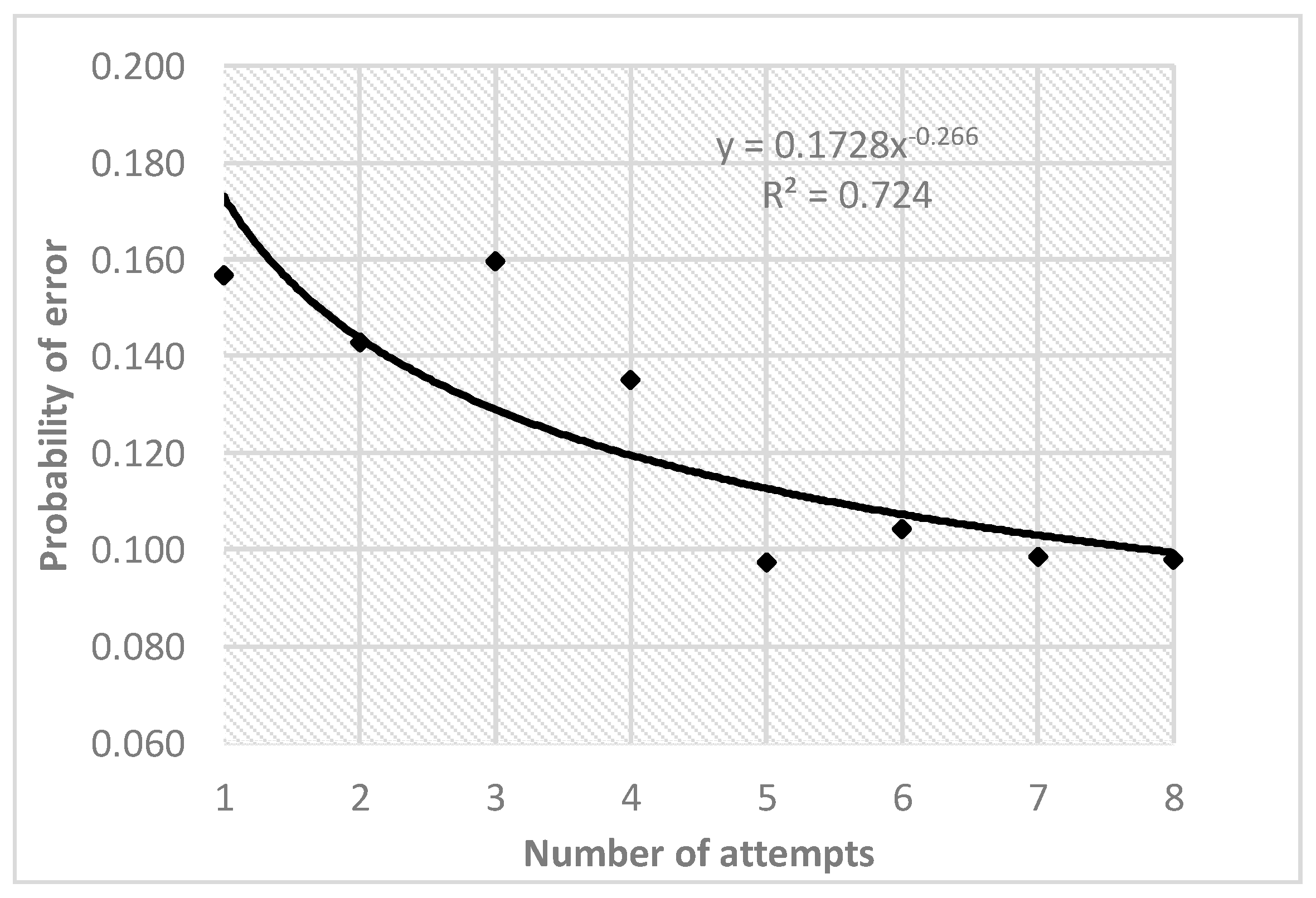
  • We conduct a small sample pilot study to show that FITS can be used to develop a deeper understanding of learning effects and knowledge acquisition based on the analysis of student models, for example, using learning curves.
FITS is developed based on the problem of classical time series decomposition. Time series decomposition allows the forecaster to understand a wide variety of patterns and behaviour exhibited by the underlying process and is typically a first step in creating any forecast [19]. This allows one to answer important questions, for example “What is the nature of the trend: increasing or decreasing?” “What is the nature of the seasonal cycle, monthly or quarterly?” “Is there a change in the structure of the underlying process?” and “Are there extreme values in the time series which may not be explainable by statistical features such as special or extreme events?”.
In Section 2, we discuss the instructional domain for FITS: the decomposed time series. We had three goals when developing FITS: (1) to provide a system which could be used in formal forecasting education and training which is more widely available at a lower cost, (2) to develop a better understanding of how individuals learn to forecast and the impact of personalised tutoring (including the type, format and nature of individual feedback) and the pedagogical strategies that work well across all individuals, and (3) by the way of above, continue to enhance our understanding for further development of forecasting education. Section 3 discusses the conceptual design of FITS using two sources: the analysis of the think-aloud protocols collected from students solving problems, and the evidence from literature, while Section 4 presents the architecture of FITS and the details of its implementation.
We conducted a pilot evaluation study over four weeks with Master-level students, presented in Section 5. The results (presented in Section 6) show that all students using the system obtained improvement in test scores. Moreover, while the number of students who completed all elements of the study is small (four students), we used learning curves to show that students were learning the underlying knowledge elements. The grouped student model obtained in the study exhibited a good fit to a power curve (R2 = 0.724) and showed a 40% decrease in the initial error probability after eight attempts, suggesting that students were acquiring the time series decomposition domain knowledge, and quickly. Further research will involve a large-scale study to evaluate additional forecasting tasks and the impact of different types of feedback, as well as provide more generalisable results.

2. Task Analysis: Decomposed Time Series

The most basic model of a decomposed time series takes two forms. The additive model assumes that seasonal variation does not interact with the trend of a time series and is as follows:
yt = St + Tt + Et
where yt is the original time series data, St is the seasonal component, Tt is the trend component, Et is the error or noise component, and t represents the time index. In contrast, the multiplicative model assumes that seasonal variation interacts with the trend component:
yt = St × Tt × Et
For a time series with seasonal period m, the seasonal component (captured in seasonal indices) is assumed constant from year to year.
Problem design required creation of a comprehensive procedural overview of the decomposition task for both additive and multiplicative decomposition. This required iteratively working through problem questions to identify various pathways to solutions. The general procedure for the additive decomposition consists of the following steps (see also Figure 1):
Construct the time series plot. This is used to evaluate patterns and behaviour in data observed over time [2].
Visually identify patterns. This step involves visual inspection of the time series plot in order to identify all time series components [20].
Calculate the centred moving average. To estimate the trend-cycle of the time series, a centred moving average (CMA) of order m must be calculated to obtain Tt. This involves identifying the frequency of the time series, e.g., monthly, quarterly, or annual. Students select between two formulas for the centred moving average depending on whether the seasonal period is odd or even. Note that other forms of moving average methods may be used at this point to isolate the trend component. The implementation of FITS will focus on the use of the centred moving average.
Calculate the de-trended time series. Subtract Tt from the original time series to get Yt − Tt = St + Et and obtain the detrended series. Students should recognise that the centred moving average provides an estimate of the trend-cycle, that is, the first component of the time series has now been estimated. By subtracting this component from the time series, what is left is the seasonal component (if one exists), and the noise/remainder component.
Check for seasonality. It is possible again to perform a second inspection of the time series for any seasonal component. If this was not identifiable in the initial time series plot or if such a plot was not performed, then it is possible to plot the de-trended time series which now has the trend-cycle removed, and in which any seasonal pattern should be more clearly visible.
Calculate the seasonal indices. Having identified the frequency of the time series and the existence of a seasonal component, estimate the seasonal index for each seasonal period i = 1, …, m by averaging all the values for that period i. For example, given monthly data the seasonal index for January is the average of all the de-trended January values in the data. The seasonal component St is then taken as the set of all seasonal indices, January to December, for each year of the data.
Combine all components of the time series. Having estimated all components of the time series, trend-cycle, seasonal indices, and remainder, each component needs to be combined. This step is necessary to calculate the noise component but is also useful for validating the quality of the previous decomposition steps.
Calculate the noise/remainder component. Finally estimate Et, the remainder component, by subtracting the estimated seasonal and trend-cycle components from the original time series, that is, Et = Yt − Tt − St.
Calculate the reconstructed time series. At this stage all components have been decomposed and obtained separately. Each can be plot separately as a time series. Combine all components trend-cycle, seasonal, and remainder to produce the reconstructed time series. This can be used to test whether the decomposition was performed correctly.
To perform the classical multiplicative decomposition, the process is similar, needing only to replace all subtractions with divisions in the additive procedure.

3. Conceptual Design

The overall design, development and deployment of the Forecasting Intelligent Tutoring System took approximately 5 months. It was informed by the forecasting literature and the analysis of data collected via the think-aloud protocol [21]. In this section we discuss each of these, and how they contributed to the design of the system.

3.1. Think Aloud Protocols Inform Pedagogy

In designing FITS, we first needed to understand the knowledge and skills required to solve each subtask as well as the interactions between various steps. This was needed to determine the student experience and interaction with the system, and how to best present various subtasks and related information to the student. In total, ten one-hour think-aloud protocols were obtained to uncover the ‘student voice’. Five students were selected from an Undergraduate Business Forecasting course, and another five from a Masters Business Forecasting course at a leading University in the UK. We asked each student to solve one problem using the classical time series decomposition method and Microsoft Excel 97-2003. We recorded each participants’ think-aloud utterances. Additionally, we made notes on their behaviour and tone of voice in relation to their progress throughout the task. The complete analysis of the protocols is the subject of ongoing research; however, the insights gained from the protocols aided in the design of FITS.

3.1.1. From Procedure to Knowledge Acquisition

It was clear from the think-aloud data that some students focused on the application of procedures rather than knowledge acquisition, which Anderson [22] shows is clearly insufficient for deep learning. A student may be able to explain precisely the sequence of steps required to decompose a time series but may still lack the awareness of the interrelationships between time series steps and components or the knowledge utilised when executing a particular step. For example, one participant initially calculated the CMA:
“So now I have- now we have, it’s meant to be divide by twelve but I put divide by two. Okay so now I have the moving average, twelve moving average er, what I do next is it is. So I think I’m going to try to take the actual data minus the moving average to, to see if there is any trend.”
In a latter step that same participant attempted to calculate the trend not recognising that the CMA provided an estimate of the trend component:
“but I haven’t got the trend so I need to calculate the trend and get the error (how to calculate trend…)”
This suggested the need for identifying subtasks at a sufficiently detailed level to target specific knowledge and skills acquisition through feedback. FITS makes these implicit actions and knowledge chunks whether known or unknown, explicit. For example, students are explicitly asked to identify the starting position where they can first calculate the CMA. This is often overlooked in classroom questions/exercises and encourages students to be aware of the business and temporal context of the time series data and time period in which the data first becomes available to perform certain calculations. Students are also asked first to identify explicitly which component should be used in a particular calculation. In calculating the seasonal matrix, students are asked to enter the number of rows and columns allowing them to test their knowledge of the time series seasonal periodicity and number of full seasons. Moreover, students are asked to identify randomly the data points in the full series which map to the seasonal matrix ensuring that students are capable of doing this mapping, which can otherwise be missed when students are provided with linked excel templates as is often the case.

3.1.2. Review and Reflection

Many steps and individual calculations are involved in the full classical decomposition of the time series. We observed that many students ran out of space within the excel spreadsheet in which to fit their solutions, and often lost track of the location of previous steps within the spreadsheet. The utterance from one student who was particularly frustrated included: “Let’s move those out of the way”, “So move those out of the way” and “So um move those columns so it’s obvious that they are columns” each coming after several key solution steps. Throughout the entire decomposition process, FITS makes previously executed steps easily available and accessible, and the visualisation of the resulting time series from such steps is available. This allows students to easily and continuously reflect on previous actions and form links with current and future steps.

3.1.3. Data Visualisation

An important requirement which resulted from analysing the collected data was the need for time series visualisation, both to help students orientate themselves to different phases of the task, and as a way of validating possible solutions. It was common to hear such phrases as “going to plot that just so I can see what it looks like”, “yeah that looks more reasonable I think” and “For my own representation I guess”. Time series data is typically presented to students as raw numerical data. Results of the protocol analysis supported the need for constant graphical visualisation of the time series data consistent with literature [20]. The use of graphical plots has been shown to assist in identifying patterns and anomalous time series observations, and providing useful insights for forecasters [2,23]. Students repeatedly visualised each derived time series component and used it as a means of validation. One participant was observed using the incorrect CMA length to remove the seasonal component, and only noticed their incorrect action after plotting the CMA:
“So I have to decide the length of the centred moving average, I can try a couple- so it could be three for example so I just calculate the average values of three, of the past series and drag this down. Okay, I must round the values down to two decimal places so I’ll do that okay there it is so that’s the moving average and I can add it to the by three. Okay right so from this graph I can see that it is definitely not smooth enough”
FITS provides explicit feedback on visualisation (often overlooked as an important step) and supports the visualisation of each newly calculated/derived series. We hope that this facilitates the behaviour in students that time series visualisation is important in terms of their orientation of the current state of the decomposition process and for the validation of previously executed steps.

3.2. Forecasting Literature Inform Design

The literature on forecasting, in particular judgmental forecasting and forecasting support systems has much to say about the design of systems for supporting better judgment and forecasting performance. Many of these studies have drawn on wider literature in psychology, systems design, and human computer interaction. In this section we review the main findings from the forecasting literature which influenced the design of FITS.

3.2.1. Feedback

We wanted FITS to provide immediate feedback to students, informing them whether their action is correct or not (outcome feedback). In the situations when students make mistakes, the feedback should inform the student about the underlying domain principles that their solution violates (cognitive feedback).
The literature supports that feedback should be both cognitive and outcome based. The study by Harvey [20] cites seven principles for improving judgement in forecasting. The third principle, ‘keep records of forecasts and use them appropriately to obtain feedback’, relates to storing and providing feedback. The study stresses the importance of outcome feedback related to the accuracy of the forecasted variable, and cognitive feedback related to persistent incorrect practice such as over-forecasting. In a study by Schmitt, Coyle and Saari [24] which asked people to make predictions of grade point average from students’ scores, the group who received outcome feedback after each prediction performed significantly better than the group that did not receive any feedback. Similarly, a study by Fischer and Harvey [25] where groups were asked to combine forecasts, found that the group which received outcome feedback was significantly better than the one which obtained no feedback. Harvey and Fischer [26] later compared outcome and cognitive feedback and found that the combination of cognitive and outcome feedback outperformed outcome feedback alone. In contrast, Tape, Kripal and Wigton [27] found that in clinical predictions and performing straightforward tasks, outcome feedback was more effective than cognitive feedback. Taken together, evidence from the literature suggests that both outcome and cognitive feedback are important in particular for complex multistep tasks such as time series decomposition. There is also evidence that feedback should be immediate. Bolger and Wright [28] found that experts perform well tasks which provide immediate outcome feedback. This is supported by decades of research into ITSs which has shown the importance of immediate and cognitive feedback to learning [10,29,30,31,32].

3.2.2. Data Availability

In the design of FITS, all data related to the time series decomposition problem is always available to the student, including the raw time series data, previously calculated steps, all previous subtasks, and all tables and graphical illustrations.
Tversky and Kahneman [33] discuss data availability, the idea that information most easily retrievable from memory will most likely be associated with particular events. This suggests that increasing the availability of information relevant to certain tasks increases recall of that event. Goldstein and Gigerenzer [34] make the distinction between recognition as a ‘binary phenomenon’ and availability as recall or familiarity, denoting levels of knowledge or experience. Both lead to the conclusion that information available to the user determines performance in various types of retrieval tasks with availability having a positive correlation in terms of speed and confidence in task execution. This is a principle built into the FITS interface and pedagogical strategy.

3.2.3. Data Visualisation

In the design of FITS, data is always presented in a dual tabular and graphical format and students can manually display any time series or time series component at any point during a session. Subcomponents when solved automatically are displayed graphically and feedback is provided at various points which remind students to visualize time series data.
Evidence suggests that errors made in time series analysis are lessened when data is presented in graphical form as compared to tabular format [20]. Angus-Leppan and Fatseas [35] observed reductions in forecast errors of up to two percent when time series data was presented as a line graph compared to when it was presented as numbers in tabular format. Forecasts of trended series presented graphically are much less biased than forecasts presented in tabular form. In eight of nine forecasts, Dickson, DeSanctis and Mcbride [36] found that participants in their study obtained more accurate forecasts when data was graphed rather than represented as tables. Other studies have reinforced the view that data should be presented in graphical form [37,38] while Harvey and Bolger [39] go further to exploring the reasons why.

4. System Design and Architecture

FITS was developed in ASPIRE, an authoring system for development of constraint-based ITSs. ASPIRE enables domain experts to develop and deploy tutors. The reader is directed to Mitrovic et al., [40] for further details of ASPIRE and the authoring process. FITS is deployed via the ASPIRE-Tutor server which consists of a number of modules based on the typical ITS architecture including the interface, pedagogical module, diagnostic module, and the student modeller. The architecture of FITS is shown in Figure 2. The interface provides functionality for student login/logout, presentation of problem and solution workspace, submission of solutions, and all necessary functionality allowing students to interact with the system. Each student’s session when using the system is managed by the session manager which maintains basic information about the session such as the selected problem and length of time in the system.
The session manager is also responsible for loading all relevant modules when needed. For example, it will pass information to the pedagogical module when a student submits a step. The pedagogical module handles all requests related to student learning and curriculum sequencing, including evaluating student’s submission and problem selection. After the student’s step is analysed, the pedagogical module provides feedback to the student. Another important module is the student modeller which maintains a long-term model of the student’s knowledge. The pedagogical module will query the student modeller in deciding the appropriate feedback to be provided based on a diagnosis of the student solution provided by the diagnostic module.

4.1. Problem Design and Knowledge Representation

We designed six additive and four multiplicative types of decomposition problems (see Appendix A). All problems were based on real world datasets freely accessible from the internet. The various time series problems were selected to encompass varying skill complexity and level of knowledge based on different properties of the time series (Table 1). Each problem varies according to the length of time series data, frequency, noise level, presence of time series components and decomposition task. These reflect differing degrees of difficulty and present different changes. Each problem was solved by three experts, using the procedural approach in Figure 1 and following the algorithms discussed in Section 2. In using the system, these three experts were able to identify pedagogical and systems interventions to further improve FITS. For example, during the testing phase, one expert provided the following feedback on the system interface:
“it’s a bit unfortunate that you can’t skip a question you can’t answer. I was blocked twice and only got lucky to find the correct answer to the first block by chance.”
Another expert commented as follows on the pedagogy and flow towards the solution: “Well, this formula looks intriguing, so I’ll choose it, and it turns out to be correct. Unfortunately, I still don’t understand it, and so I’m completely blocked at the next question”.
A comprehensive set of feedback reports was received from these experts and used to improve FITS. In FITS, students are able to select a problem to work on from the set of ten questions.
FITS is a constraint-based tutor [15,30], meaning that the knowledge required to solve problems is represented in the form of constraints [30,40,41,42]. Domain knowledge is a collection of constraints or state descriptions of the general form:
If <relevance condition> is true, then <satisfaction condition> had better also be true, otherwise something has gone wrong.
The relevance condition specifies the parts of the student solution which must be matched in order that the constraint is triggered. The satisfaction condition specifies the part of the student solution which must be satisfied if the corresponding relevance condition is matched [15,16]. An example of a FITS constraint is:
IF the current step is to estimate the noise AND the problem uses additive decomposition THEN the formula must use subtraction.
Given this constraint, the student modeller responds as follows:
(a)
If the student was not working on the Noise Estimation step and the problem does not use additive decomposition, then the constraint would not be triggered (i.e., not relevant for this submission).
(b)
If the student was working on the Noise Estimation step, and the problem uses additive decomposition, then the constraint would be triggered (i.e., relevant for this submission). From here:
  • If the student’s answer uses subtraction, then the constraint is recorded as being satisfied (i.e., the student has correctly carried out this concept).
  • If the student’s answer does not use subtraction, then the constraint is recorded as being violated (i.e., the student has not carried out or incorrectly carried out this concept).
The job of the student modeller is to generate and maintain a complete model of the student’s knowledge as represented by constraints. Violated constraints indicate which knowledge elements students are struggling to grasp. Each constraint has attached feedback messages, which are given to the student when the constraint is violated. The current version of FITS contains 43 constraints. This is likely to increase as the number of problems and the curriculum supported expands.

4.2. Student Interface

The FITS interface is developed in the standard web languages of HTML, JavaScript, and CSS, and consists of five panes. A screenshot is shown in Figure 3. The interface is designed to allow students to have access to and visualise the full process from the original time series through to the individual components of the decomposed series, as described in Figure 1. At the top of the page is the task pane, which shows the problem description. This description is always visible as an easy point of reference for the learner. Below problem text is the spreadsheet workspace, where all spreadsheet data is displayed, updated, and can be selected. The interface was designed to replicate the look and functionality of a spreadsheet, while further functionality was added to make the interface behave more spreadsheet-like (for example, providing basic formula support). The main motivation for this design decision was the widespread use of Excel in business forecasting course and in practice. Both the raw data and derived data series, such as when calculating the centred moving average or the detrended series, are available in the spreadsheet workspace. This allows learners to see how the data changes over time based on their actions.
The visualisations pane, located at the centre bottom panel, shows the plotted graphs. These may be automatically plotted or generated manually by the student, and any graphs generated go into a list to be viewed at any point during this problem. The visualisations pane also provides a mini spreadsheet (in a separate tab) to calculate the seasonal layout. This design decision is again consistent with our findings from analysing the think-aloud data (Section 3.1) on the importance of graphical visualisation of time series data for problem orientation and solution validation. The use of graphical plots has been shown to assist in identifying patterns and anomalous time series observations, and providing useful insights for forecasters [2,23]. Students repeatedly visualised each derived time series component and used it as a means of validation. One participant was observed using the incorrect CMA length to remove the seasonal component, and only noticed their incorrect action after plotting the CMA; see below:
“So I have to decide the length of the centred moving average, I can try a couple- so it could be three for example … Okay right so from this graph I can see that it is definitely not smooth enough”
Directly below the workspace pane are three additional panes. The leftmost pane is the current question pane, which contains the subtask that the student is currently working on, and all previous subtasks that the learner has completed so far in the problem. Student think-aloud protocols suggested the need for identifying subtask at sufficiently detailed level to target specific knowledge and skills acquisition. FITS makes these actions and knowledge chunks explicit. For example, students are explicitly asked to identify the starting position where they can first calculate the CMA. This is often overlooked in classroom questions/exercises and encourages students to be aware of the business and temporal context of the time series data and time period in which the data first becomes available to perform certain calculations.
The bottom rightmost pane is the feedback pane. When the learner answers the current subtask, they may receive feedback on their solution by clicking the ‘Check’ button. The solution is passed to the server, where it is checked against the constraints within the domain model and evaluated to either be correct or incorrect. If incorrect, FITS also returns fine-grained feedback about exactly which parts of the solution are incorrect and the violated domain principles, which correspond to violated constraints.

4.3. Feedback

The feedback provided by FITS is both cognitive- and outcome-based as supported by decades of research into ITSs which has shown the importance of immediate and corrective feedback to learning [10,22,31]. FITS has two types of constraints: syntax constraints which check the syntax of the student solution, e.g., a number is provided and not a letter, and semantic constraints, which check that the student’s solution is correct—that is, it answers the question. To support feedback, each constraint is associated with two feedback messages, shown to the student one at a time: initially when the constraint is violated, and then again if the student request further feedback. The progression of feedback goes over several levels:
  • Quick Check, specifying whether the answer is correct or not;
  • Error Flag, identifying only the part of the solution that is erroneous;
  • Hint, identifying the first error and providing information about the domain principle that is violated by the student’s solution;
  • Detailed Hint (a more detailed version of the hint);
  • All Errors (hints about all errors);
  • Show Solution.
FITS starts with Quick Check and progresses with each consecutive submission of the same problem to Detailed Hint unless a specific type of feedback is requested. The last two feedback levels are only available on student request.

5. Pilot Study

5.1. Experiment Design

The study involved Masters-level Business students from a leading university in the UK, enrolled in the 10-week course on Business Forecasting. The students had prior knowledge of business and statistics, from other courses within the MSc and prior education.
We adopted the pre-post test experiment design. Pre-post test designs allow us to measure how much students learnt from using FITS. Data was collected over a four-week period from the beginning of the course. In Week 1, students sat the pre-test, after receiving the lecture and tutorial session on time series decomposition delivered over 4 h. The students were taught to decompose time series using the same approach outlined in Section 2, and to perform both additive and multiplicative decomposition. The pedagogical approach in teaching students this material involved the use of an Excel spreadsheet model with a guided example on time series decomposition, as outlined in Section 2. This ensured that students were taught the same decomposition methodology and content as that used in FITS. However, there were no restrictions on the pedagogy adopted in class. The key requirement was that students be able to perform and show knowledge of classical time series decomposition as outlined in Section 2.
Students used FITS in weeks 2 and 3 of the course with no further academic intervention. That is, during this period the only formal support received on time series decomposition was provided by FITS. During these two weeks, students had access to the system online and anytime. Finally, in Week 4, students were asked to complete the post-test.

5.2. Pre- and Post-Test

Using pre- and post-tests allows us to measure the learning effectiveness of FITS by comparing what the student knew before and after the study. The tests consisted of a decomposition exercise requiring students to answer several key questions related to a given time series dataset. Students had the option of solving the problem by hand or via the use of Excel, with all students opting to use Excel. The tests consist of a similar set of questions in the same format and of the same level of difficulty (Appendix B). While there are no standardized tests associated with the domain of knowledge, the questions included are standard to assessing the application of time series decomposition using the classical approach, and as taught to students in the course. These questions assess students’ ability to calculate estimates for the various components of the decomposition—for example, the seasonal indices, but also knowledge of the length of centred moving average to be used. While tests may be criticised for mainly measuring student’s ability to retain and recall known facts, results of pre- and post-tests together with student models and learning logs obtained from FITS provide increased evidence of whether there are actual improvements in performance.

5.3. Sample Size

Student participation in the study was completely voluntary. Out of 70 students enrolled in the course, 17 students completed the pre-test and nine students attempted the post-test. Eight students used FITS. Of these students, four students completed all parts of the study (i.e., pre-test, use of FITS and the post-test). Consequently, the analysis proceeds with these four students. It should be noted that one student logged into FITS but had no meaningful interaction. Having logged into FITS and completed pre- and post-tests, this student is still included. The reason for lack of participation of students was due to lack of integration of FITS into the summative assessment, and an overload of other assessments during the evaluation period. We do not believe however that this undermines the contributions of the study as it provides an innovative approach to learning support in forecasting, lessons learnt during the process of creating the system, proof of concept of its application, and proof of its use in understanding student learning using student models and learning curves.

6. Data Analysis

6.1. Pre- and Post-Test

Results of the pre- and post-test, presented in Table 2, provide descriptive statistics on the scores received by the students in the pre- and post-tests. The tests were marked out of total of 15. The minimum scores were found to be 3 and 4, and the maximum scores to be 9 and 15, respectively. Students scored on average lower in the pre-test (mean score = 5.75) than in the post-test (mean score = 7.11). Closer inspection of the data revealed that three of the four students scored higher on the post-test than they did on the pre-test. The one student not showing any improvement was Participant 4 who logged into the system but did not attempt any problems. While there is an insufficient sample to generalise these findings, they do provide some indication that the system is effective in improving students’ performance.
Table 3 presents the summary data from the system. Three students used nearly all constraints in FITS, 43 being the maximum, while Participant 4 used no constraints indicating they had not submitted any solutions for evaluation of pre-post test scores of this participant show no improvement. In contrast, participants 1 and 3 who used all constraints improved substantially in their post-test scores. Participant 2 achieved notable improvement, who although attempting only one problem and triggering nearly all constraints, saw a large increase in test score from 3 in the pre-test to 15 in post-test. This participant spent 15.95 min per problem, compared to 8.72 min by Participant 1 and 11.03 min by Participant 3. This would suggest that the type of problems, constraints triggered and time per question is as equally important as overall time in the system. Overall, the participants who solved at least one problem and spent some time using the system showed an improvement in test scores.

6.2. Student Models

The student modeller maintains a long-term model of each individual student. This model contains a history of usage of every constraint found relevant for the student’s submissions. This provides a measure of the knowledge being acquired by the student throughout the tutoring journey [15,41]. In this section, we present our analysis of how students acquire constraints using learning curves. A learning curve allows the modelling of a student’s rate of learning based on CBM modelling. The horizontal axis shows the number of times a constraint is relevant and evaluated for correctness, while the vertical axis shows the probability of the student making an error (violating the constraint) on a given attempt. As an illustration, Figure 4 shows the learning curve for Participant 1. At 1 attempt, all 43 constraints are included, that is, each constraint was triggered at least once by this student and the probability of an error is 0.16. We stop at 13 attempts because at that point only 10 constraints have been triggered, and the probability of the student making an error is 0.042. We see from the fitted curve that while the learning rate (0.47) is not very high for this student (exponent of the power curve equation), there is a substantial drop in the initial error probability from 0.16 to 0.03 in only 5 attempts suggesting that the student is learning quickly, albeit with the error probability levelling off.
We repeat this analysis across all six students who solved problems in FITS to produce an aggregate learning curve. The minimal number of attempts per student was 16, where an attempt is submitting a solution for a subtask. The graph shown in Figure 5 includes constraints which have been attempted at least 8 times by all 6 students. The data exhibits a good fit to a power curve with an R2 of 0.724, suggesting that FITS did support the effective learning of constraints. The initial error probability of 0.15 drops very quickly to 0.098 after eight attempts, a 40% decrease showing that students are acquiring the time series decomposition domain knowledge quickly.
While these results are over a small number of students, they do show the potential of FITS for not only student tutoring, but also for assessing and measuring the effect of the system on student learning and knowledge acquisition. Future studies involving larger number of students will provide more generalizable results. Note that it is also possible to analyse specific constraints to assess student difficulty in grasping specific principles of the domain. This will lead to identifying areas of the domain which are particularly difficult and require further attention.

7. Conclusions

With forecasting and demand planning becoming an increasingly important requirement for business, there continues to be a need for trained and highly skilled experts. This is in addition to increasing demands within the tertiary education sector putting a strain on traditional classroom-based approaches. In this work we provide a possible solution for achieving one-to-one human-like tutoring in classical time series decomposition through the use of a computer-based ITS. This is to our knowledge the first ever intelligent tutoring system for forecasting, which provides forecasting training that is individually tailored to the learner. The system is aptly named FITS for Forecasting Intelligent Tutoring System. We described the process of developing FITS, including the conceptual design, problem construction and solution pathways, as well as the construction of the online problem-solving environment and student interface. This was aided by student think-aloud protocols through which we were able to identify situations that presented key challenges to students, and through review of prior research on forecasting support and support systems.
The main limitation of our research is the small set of participants who interacted with FITS. Although the results of our pilot study are not generalizable, they do suggest the potential for the system to improve student learning. Three students who interacted with FITS and complete pre-post tests showed improvements in learning. It was also shown how FITS facilitates the deeper understanding and knowledge acquisition by individual students and across a group of students based on the availability of student models and the analysis of such models using learning curves.
Perhaps the biggest benefit of FITS is the ability for students to practice classical time series decomposition problem-solving tasks with access to immediate and individualised feedback independent of teaching staff, independent of their location and at any time they wish to do so. Future planned work will focus on extending the system’s functionality in terms of number and types of problems covered. We also plan to conduct a large-scale study involving third-year undergraduate students from two universities in the United Kingdom. Having more data from student interactions with FITS will allow us to explore student models to understand the impact of receiving individual tutoring (including the type, format, and nature of individual feedback) and pedagogical strategies that work well across all individuals. We also plan to collect subjective opinions of students regarding various features of FITS, which will enable us to further improve the system. Finally, since FITS makes decisions based on AI, we plan to add explanations of how those decisions are made. Such explanations, referred to Explainable AI (XAI) are now starting to appear in AI-based systems, and have been shown to increase users’ trust in the system [43,44,45]. We believe that adding XAI to FITS will increase the students’ engagement with the system, resulting in higher learning.

Author Contributions

D.B.: project administration; conceptualization, supervision, methodology, investigation, software, visualization, writing—original draft; A.M.: conceptualization, supervision, methodology, investigation, software, writing—review and editing; J.H.: conceptualization, methodology, software, writing—review and editing; M.A.: conceptualization, writing—review and editing; N.K.: conceptualization, methodology, writing—review and editing. All authors have read and agreed to the published version of the manuscript.

Funding

This research was funded by Coventry University Pump Prime Research Grant Scheme 2015.

Data Availability Statement

All datasets associated with this study are not publicly available as part of measures to protect the confidentiality of participants. However, the data that support the findings of this study are available from the corresponding author upon reasonable request.

Conflicts of Interest

The authors declare no conflict of interest.

Appendix A. Problem Set

1.
Passenger Airline
The following is the classis Box and Jenkins time series of monthly totals of international airline passengers between January 1957 and December 1960. Using the classical time series decomposition method, provide the additive decomposition of the time series into its individual components.
2.
Boulder Temperatures
The following is a time series containing the average monthly temperatures for Boulder, Colorado, from January 2004 to December 2007. Using the classical time series decomposition method, provide the additive decomposition of the time series into its individual components.
3.
Crude Oil Price
The time series below contains observations from January 2007 to December 2010 measuring the price of crude oil. Using the classical time series decomposition method, provide the multiplicative decomposition of the time series into its individual components.
4.
S&P 500
Data for the SAP 500 index is given for the period from January 1996 to December 1999. Using the classical time series decomposition method, provide the multiplicative decomposition of the time series into its individual components.
5.
US GDP
The time series gives the quarterly value of the U.S. gross domestic product (billions of dollars) from 2005 to 2008. Using the classical time series decomposition method, provide the additive decomposition of the time series into its individual components.
6.
Google
The following time series contains data on the monthly volume of trading in Google stock (millions of shares) from May 2006 to January 2009. Using the classical time series decomposition method, provide the multiplicative decomposition of the time series into its individual components.
7.
Housing Starts
The data provided relate to the monthly housing starts (in thousands, seasonally adjusted) from January 2001 through December 2004. Using the classical time series decomposition method, provide the additive decomposition of the time series into its individual components.
8.
Netflix
Using the classical time series decomposition method, provide the additive decomposition of the Netflix quarterly sales data for the period 2006Q1 to 2009Q4 given below.
9.
Australian Beer Production
The following data records observations of quarterly beer production in Australia (megalitres) from 1990 to 1993. Using the classical time series decomposition method, provide the additive decomposition of the time series into its individual components.
10.
Unemployment Rate
The following is a time series of the unemployment rate for all persons aged 15–64 living in Greece. Using the classical time series decomposition method, provide the multiplicative decomposition of the time series into its individual components.

Appendix B. Pre- and Post-Tests

Appended B.1. Pre-Test

Table A1. Australia monthly production of electricity (Millions Kilowatt-hours) from January 1956 to December 1960. The following data provides monthly observations of the Australian production of electricity (Millions Kilowatt-hours) from January to December 1960.
MSCI 523: Forecasting
Pre-Test Classical Time Series Decomposition
Student ID# ______________________
(Please note that the outcome of this test is used for research purposes only and is in no way linked to the grades within this course)
DateValueDateValueDateValue
January-561254January-581497January-601721
February-561290February-581463February-601752
March-561379March-581648March-601914
April-561346April-581595April-601857
May-561535May-581777May-602159
June-561555June-581824June-602195
July-561655July-581994July-602287
August-561651August-581835August-602276
September-561500September-581787September-602096
October-561538October-581699October-602055
November-561486November-581633November-602004
December-561394December-581645December-601924
January-571409January-591597
February-571387February-591577
March-571543March-591709
April-571502April-591756
May-571693May-591936
June-571616June-592052
July-571841July-592105
August-571787August-592016
September-571631September-591914
October-571649October-591925
November-571586November-591824
December-571500December-591765
Answer the following questions assuming that your task is to perform an additive decomposition of the above time series data using the classical method.
  • Does the time series contain trend?
  • Does the time series contain seasonality?
  • What is the required length of the centred moving average?
  • In which period are you first able to calculate the centred moving average (use the same date format given in the above e.g., December-89)?
  • What is the value (to 2 decimal places) of the centred moving average for the period February-58?
  • What is the value (to 2 decimal places) of the de-trended time series for the period August-58?
  • What is the value of the seasonal index (to 2 decimal places) for the month of January?
  • What is the value (to 2 decimal places) of the noise series for the period December-59?

Appended B.2. Post-Test

Table A2. UK consumer expenditure March 1971 to December 1975. The following data provides quarterly observations on real consumers’ expendi-ture in the UK over the period March 1971 to July 1975.
MSCI 523: Forecasting
Post-Test Classical Time Series Decomposition
Student ID# ______________________
(Please note that the outcome of this test is used for research purposes only and is in no way linked to the grades within this course)
QuarterDateValueQuarterDateValueQuarterDateValue
Q1March-716855Q1March-737539Q1March-757735
Q2June-717335Q2June-737948Q2June-757984
Q3September-717467Q3September-738157Q3September-758045
Q4December-717952Q4December-738691Q4December-758646
Q1March-727147Q1March-747601Q1
Q2June-727636Q2June-747985Q2
Q3September-727829Q3September-748186Q3
Q4December-728332Q4December-748798Q4
Answer the following questions assuming that your task is to perform an additive decomposition of the above time series data using the classical method.
  • Does the time series contain trend?
  • Does the time series contain seasonality?
  • What is the required length of the centred moving average?
  • In which period are you first able to calculate the centred moving average (use the same date format given in the above)?
  • What is the value (to 2 decimal places) of the centred moving average for the period March-72?
  • What is the value (to 2 decimal places) of the de-trended time series for this same period, that is, March-72?
  • What is the value of the seasonal index (to 2 decimal places) for the Quarter ending March, that is, Q1?
  • Based upon examination of the seasonal index numbers, are expenditures seasonal? Explain.

References

  1. Syntetos, A.A.; Babai, Z.; Boylan, J.E.; Kolassa, S.; Nikolopoulos, K. Supply chain forecasting: Theory, practice, their gap and the future. Eur. J. Oper. Res. 2016, 252, 1–26. [Google Scholar] [CrossRef]
  2. Ord, K.; Fildes, R. Principles of Business Forecasting; Cengage Learning: Boston, MA, USA, 2012. [Google Scholar]
  3. Fildes, R.; Goodwin, P.; Lawrence, M. The design features of forecasting support systems and their effectiveness. Decis. Support Syst. 2006, 42, 351–361. [Google Scholar] [CrossRef]
  4. Fildes, R.; Nikolopoulos, K.; Crone, S.F.; Syntetos, A.A. Forecasting and operational research: A review. J. Oper. Res. Soc. 2008, 59, 1150–1172. [Google Scholar] [CrossRef]
  5. Armstrong, J.S. Principles of Forecasting: A Handbook for Researchers and Practitioners; Springer Science & Business Media: Berlin, Germany, 2001; Volume 30. [Google Scholar]
  6. Aleven, V.; Rowe, J.; Huang, Y.; Mitrovic, A. Domain modeling for AIED systems with connections to modeling student knowledge: A review. In Handbook of Artificial Intelligence in Education; Edward Elgar Publishing: Northampton, MA, USA, 2023; pp. 127–169. [Google Scholar]
  7. Carbonell, J.R. AI in CAI: An artificial-intelligence approach to computer-assisted instruction. IEEE Trans. Man-Mach. Syst. 1970, 11, 190–202. [Google Scholar] [CrossRef]
  8. Elsom-Cook, M. Design Considerations of an Intelligent Tutoring System for Programming Languages; University of Warwick: Warwick, UK, 1984. [Google Scholar]
  9. McCalla, G. The history of artificial intelligence in education—The first quarter century. In Handbook of Artificial Intelligence in Education; Edward Elgar Publishing: Northampton, MA, USA, 2023; pp. 10–29. [Google Scholar]
  10. Koedinger, K.R.; Anderson, J.; Hadley, W.H.; Mark, M.A. Intelligent tutoring goes to school in the big city. Int. J. Artif. Intell. Educ. 1997, 8, 30–43. [Google Scholar]
  11. Conati, C.; Merten, C. Eye-tracking for user modeling in exploratory learning environments: An empirical evaluation. Knowl.-Based Syst. 2007, 20, 557–574. [Google Scholar] [CrossRef]
  12. VanLehn, K.; Lynch, C.; Schulze, K.; Shapiro, J.A.; Shelby, R.; Taylor, L.; Treacy, D.; Weinstein, A.; Wintersgill, M. The Andes physics tutoring system: Lessons learned. Int. J. Artif. Intell. Educ. 2005, 15, 147–204. [Google Scholar]
  13. Azevedo, R.; Taub, M.; Mudrick, N.V. Using multi-channel trace data to infer and foster self-regulated learning between humans and advanced learning technologies. In Handbook of Self-Regulation of Learning and Performance; Schunk, D., Greene, J.A., Eds.; Routledge: New York, NY, USA, 2018; pp. 254–270. [Google Scholar]
  14. Graesser, A.C.; Hu, X.; Nye, B.; VanLehn, K.; Kumar, R.; Heffernan, C.; Heffernan, N.; Woolf, B.; Olney, A.M.; Rus, V.; et al. ElectronixTutor: An intelligent tutoring system with multiple learning resources for electronics. Int. J. STEM Educ. 2018, 5, 15. [Google Scholar] [CrossRef]
  15. Mitrovic, A.; Ohlsson, S. Evaluation of a Constraint-Based Tutor for a Database Language. Int. J. Artif. Intell. Educ. 1999, 10, 238–256. [Google Scholar]
  16. Mitrovic, A.; Ohlsson, S.; Barrow, D.K. The effect of positive feedback in a constraint-based intelligent tutoring system. Comput. Educ. 2013, 60, 264–272. [Google Scholar] [CrossRef]
  17. Kern, T.; McGuigan, N.; Mitrovic, A.; Najar, A.S.; Sin, S. iCFS: Developing Intelligent Tutoring Capacity in the Accounting Curriculum. Int. J. Learn. High. Educ. 2014, 20, 91. [Google Scholar]
  18. Mitrovic, A.; McGuigan, N.; Martin, B.; Suraweera, P.; Milik, N.; Holland, J. Authoring Constraint-based Tutors in ASPIRE: A Case Study of a Capital Investment Tutor. In Proceedings of EdMedia: World Conference on Educational Media and Technology 2008; Luca, J., Weippl, E.R., Eds.; Association for the Advancement of Computing in Education (AACE): Vienna, Austria, 2008; pp. 4607–4616. [Google Scholar]
  19. Makridakis, S.; Wheelwright, S.C.; Hyndman, R.J. Forecasting: Methods and Applications, 3rd ed.; Wiley India Pvt. Limited: Hoboken, NJ, USA, 2008. [Google Scholar]
  20. Harvey, N. Improving judgment in forecasting. In Principles of Forecasting; Springer: Berlin/Heidelberg, Germany, 2001; pp. 59–80. [Google Scholar]
  21. Ericsson, K.A.; Simon, H.A. Protocol Analysis: Verbal Reports as Data, Revised ed.; MIT Press: Cambridge, MA, USA, 1993. [Google Scholar]
  22. Anderson, J.R. Problem solving and learning. Am. Psychol. 1993, 48, 35. [Google Scholar] [CrossRef]
  23. Hyndman, R.J.; Athanasopoulos, G. Forecasting: Principles and Practice; OTexts: Melbourne, Australia, 2014. [Google Scholar]
  24. Schmitt, N.; Coyle, B.W.; Saari, B.B. Types of task information feedback in multiple-cue probability learning. Organ. Behav. Hum. Perform. 1977, 18, 316–328. [Google Scholar] [CrossRef]
  25. Fischer, I.; Harvey, N. Combining forecasts: What information do judges need to outperform the simple average? Int. J. Forecast. 1999, 15, 227–246. [Google Scholar] [CrossRef]
  26. Harvey, N.; Fischer, I. Development of experience-based judgment and decision making: The role of outcome feedback. In The Routines of Decision Making; Psychology Press: London, UK, 2005; pp. 119–137. [Google Scholar]
  27. Tape, T.G.; Kripal, J.; Wigton, R.S. Comparing methods of learning clinical prediction from case simulations. Med. Decis. Mak. 1992, 12, 213–221. [Google Scholar] [CrossRef] [PubMed]
  28. Bolger, F.; Wright, G. Assessing the quality of expert judgment: Issues and analysis. Decis. Support Syst. 1994, 11, 1–24. [Google Scholar] [CrossRef]
  29. Anderson, J.R.; Corbett, A.T.; Koedinger, K.R.; Pelletier, R. Cognitive tutors: Lessons learned. J. Learn. Sci. 1995, 4, 167–207. [Google Scholar] [CrossRef]
  30. Mitrovic, A. Fifteen years of constraint-based tutors: What we have achieved and where we are going. User Model. User-Adapt. Interact. 2012, 22, 39–72. [Google Scholar] [CrossRef]
  31. Mitrovic, A.; Suraweera, P.; Martin, B.; Weerasinghe, A. DB-suite: Experiences with three intelligent, web-based database tutors. J. Interact. Learn. Res. 2004, 15, 409. [Google Scholar]
  32. Du Boulay, B. Recent meta-reviews and meta–analyses of AIED systems. Int. J. Artif. Intell. Educ. 2016, 26, 536–537. [Google Scholar] [CrossRef]
  33. Tversky, A.; Kahneman, D. Judgment under uncertainty: Heuristics and biases. In Utility, Probability, and Human Decision Making; Springer: Berlin/Heidelberg, Germany, 1975; pp. 141–162. [Google Scholar]
  34. Goldstein, D.G.; Gigerenzer, G. The recognition heuristic: How ignorance makes us smart. In Simple Heuristics That Make Us Smart; Oxford University Press: Oxford, UK, 1999; pp. 37–58. [Google Scholar]
  35. Angus-Leppan, P.; Fatseas, V. The forecasting accuracy of trainee accountants using judgemental and statistical techniques. Account. Bus. Res. 1986, 16, 179–188. [Google Scholar] [CrossRef]
  36. Dickson, G.W.; DeSanctis, G.; McBride, D.J. Understanding the effectiveness of computer graphics for decision support: A cumulative experimental approach. Commun. ACM 1986, 29, 40–47. [Google Scholar] [CrossRef]
  37. Lawrence, M.J.; Edmundson, R.H.; O’Connor, M.J. An examination of the accuracy of judgmental extrapolation of time series. Int. J. Forecast. 1985, 1, 25–35. [Google Scholar] [CrossRef]
  38. Lawrence, M.J. An exploration of some practical issues in the use of quantitative forecasting models. J. Forecast. 1983, 2, 169–179. [Google Scholar] [CrossRef]
  39. Harvey, N.; Bolger, F. Graphs versus tables: Effects of data presentation format on judgemental forecasting. Int. J. Forecast. 1996, 12, 119–137. [Google Scholar] [CrossRef]
  40. Mitrovic, A.; Martin, B.; Suraweera, P.; Zakharov, K.; Milik, N.; Holland, J.; McGuigan, N. ASPIRE: An authoring system and deployment environment for constraint-based tutors. Int. J. Artif. Intell. Educ. 2009, 19, 155–188. [Google Scholar]
  41. Ohlsson, S. Learning from performance errors. Psychol. Rev. 1996, 103, 241. [Google Scholar] [CrossRef]
  42. Ohlsson, S. Constraint-based student modeling. J. Artif. Intell. Educ. 1992, 3, 429–447. [Google Scholar]
  43. Conati, C.; Barral, O.; Putnam, V.; Rieger, L. Toward personalized XAI: A case study in intelligent tutoring systems. Artif. Intell. 2021, 298, 103503. [Google Scholar] [CrossRef]
  44. Khosravi, H.; Shum, S.B.; Chen, G.; Conati, C.; Tsai, Y.S.; Kay, J.; Knight, S.; Martinez-Maldonado, R.; Sadiq, S.; Gašević, D. Explainable Artificial Intelligence in education. Comput. Educ. Artif. Intell. 2022, 3, 100074. [Google Scholar] [CrossRef]
  45. Mullins, R.; Conati, C. Enabling understanding of AI-Enabled Intelligent Tutoring Systems. In Design Recommendations for Intelligent Tutoring Systems: Volume 8—Data Visualization; US Army Combat Capabilities Development Command–Soldier Center: Natick, MA, USA, 2020; pp. 141–148. [Google Scholar]
Figure 1. Task analysis of classical time series decomposition.
Forecasting 06 00012 g001
Figure 2. Architecture of FITS Tutor on ASPIRE.
Forecasting 06 00012 g002
Figure 3. FITS student interface.
Forecasting 06 00012 g003
Figure 4. Learning curve for Participant 1.
Forecasting 06 00012 g004
Figure 5. Learning curve for FITS.
Forecasting 06 00012 g005
Table 1. Time series problem characteristics by question.
QuestionLengthFrequencyNoiseTrendSeasonalityDecomposition
Airline passenger48MonthlyLowYesYesAdditive
Boulder48MonthlyLowNoYesAdditive
Crude Oil48MonthlyStructural ChangeNoNoMultiplicative
S&P 50048MonthlyOutlierYesNoMultiplicative
US GDP16QuarterlyOutlierYesNoAdditive
Google33MonthlyHighNoNoMultiplicative
Housing Starts48MonthlyMediumYesNoAdditive
Netflix16QuarterlyLowYesNoAdditive
Australian Beer
Production
16QuarterlyLowYesYesAdditive
Unemployment Rate16QuarterlyLowYesYesMultiplicative
Table 2. Pre- and Post-test for participants completing entire study.
Pre-TestPost-Test
Number of students44
Minimum score34
Maximum score915
Mean5.757.11
Median5.513.5
Standard Deviation2.755.20
Table 3. Student summary data generated from FITS.
Constraints UsedSolved ProblemsMessagesTime (Mins)Pre-TestPost-Test
Participant 1431014087.23915
Participant 23812615.95315
Participant 34310144110.38712
Participant 40002.0544
Disclaimer/Publisher’s Note: The statements, opinions and data contained in all publications are solely those of the individual author(s) and contributor(s) and not of MDPI and/or the editor(s). MDPI and/or the editor(s) disclaim responsibility for any injury to people or property resulting from any ideas, methods, instructions or products referred to in the content.

