Ecological Forecasting and Operational Information Systems Support Sustainable Ocean Management

Abstract

In times of rapid change and rising human pressures on marine systems, information about the future state of the ocean can provide decision-makers with time to avoid adverse impacts and maximise opportunities. An ecological forecast predicts changes in ecosystems and its components due to environmental forcing such as climate variability and change, extreme weather conditions, pollution, or habitat change. Here, we summarise examples from several sectors and a range of locations. We describe the need, approach, forecast performance, delivery system, and end user uptake. This examination shows that near-term ecological forecasts are needed by end users, decisions are being made based on forecasts, and there is an urgent need to develop operational information systems to support sustainable ocean management. An operational information system is critical for connecting to decision makers and providing an enduring approach to forecasting and proactive decision making. These operational systems require significant investment and ongoing maintenance but are key to delivering ecological forecasts for societal benefits. Iterative forecasting practices could provide continuous improvement by incorporating evaluation and feedback to overcome the limitations of the imperfect model and incomplete observations to achieve better forecast outcomes and accuracy.

1. Introduction

Oceans are changing rapidly, with hotspots of long-term ocean warming [1] and increased frequency of extreme events (e.g., marine heatwaves, [2]) impacting marine species and habitat quality, distribution, structure, and function (e.g., [3]). Major impacts on coastal habitats have been recorded around the world [4,5], as have large-scale shifts in species distribution [6,7] and abundance (e.g., [8]). The combination of rapid ocean change with increasing pressure from human activities and use of marine spaces for new industries associated with the Blue Economy [9] means that historical expectations for ecological conditions may not be realised in the future. This will make ocean use and management more challenging than in the past unless new tools and approaches for ecological forecasting can be provided and operational information systems developed.

Many sectors can benefit from ecological forecasts [10], (Ecological Forecast Initiative https://ecoforecast.org/ (accessed on 1 December 2022)), which can lower the risk of management failure under global change [11] on both short- and long-term scales [12]. Ecological forecasts, commonly referred to as “ecoforecasts”, can deliver predictions of abundance, distribution, and phenology for single species, multispecies, or communities, or predictions of ecological events such as harmful algal blooms, pathogen loads, hypoxic conditions, and shifts in species and habitats under climate change (https://oceanservice.noaa.gov/ecoforecasting/noaa.html (accessed on 1 December 2022); [10,13]). These forecasts can be for a range of time scales, from nowcasts through to seasonal and climate scales [14,15], and tend to be at local (~10 km) to regional spatial scales (~100 km). Ecosystem-based approaches to management (such as the Ecosystem Approach, Ecosystem-based Management, Ecosystem-based Fisheries Management, Nature-based Solutions, etc), which are being practiced in a multitude of settings around the world, could benefit from forecasts of vital ecosystem indictors and/or valued services/threats [16].

Forecasts can provide information on large and difficult-to-observe ecosystems to support the effective managers of iconic habitats such as the Great Barrier Reef. Forecasts could support the application of Integrated Pest Management (e.g., the crown-of-thorns starfish) and increase the preparation time for managers. Ecological forecasts can also reduce the risk to human life to offer a great benefit to society, just as weather or storm forecasts have been widely adopted by coastal and offshore vessel captains. Studies have shown there are statistically significant patterns between environmental drivers and hazardous marine species, e.g., significant patterns do occur for shark and crocodile attacks and Irukandji stings on humans (e.g., [17,18,19]). Therefore, forecasts of environmental conditions could provide the likelihood of occurrences of marine hazards to humans.

Early marine ecological forecasts were developed for fisheries applications rather than for conservation or tourism. These forecasts have been used in decision-making systems for management, e.g., forecasts of the distribution of southern bluefin tuna habitat off the east coast of Australia [20] and leatherback turtles off the Hawaiian Islands [21], which have been expanded to other pelagic species and regions [22]. The first marine ecoforecast systems have been developed in Australia [23] and North America (e.g., [24,25,26]), and there are a few examples from elsewhere [22,27]. However, there has been a large increase in ecological forecasts over the years and they now cover marine, fresh water and terrestrial ecosystems over all seven continents [22,28].

Although there has been a science push for some of these applications, end-user demand for information has also contributed to uptake. Realizing the full potential of marine ecological forecasting will require bridging the gaps between marine ecology and oceanographic modelling on the one hand, and between science and end-users on the other [22]; this will require improved information delivery systems. Although ecological forecasts often depend on physical forecasting capability, such as dynamical ocean model forecasts, these often feed into statistical approaches and other types of modelling. Ecological forecasts also include single species models widely used to generate short-term abundance forecasts based on population dynamics, and often do not use environmental data. These population models are used widely in fisheries [29] and we do not cover them here.

To apply ecological forecasting for management decision support, operational information systems have been developed to integrate comprehensive interoperable information and modelling platforms. These systems provide government agencies and industries access to improved environmental information (e.g., [30,31]; NOAA Ecoforecasting). An operational information system usually integrates data with marine models (which may include physical and socioecological models), visualisation, reporting, and decision support tools for management options. An example of such a system is shown in Figure 1, where users can access a range of decision support information through a web-based dashboard, such as forecasts (of disease outbreaks, extreme events, climate change and economic shocks), risk and strategic assessments, reports from farm status to compliance status, incidence response, and guidance and documentation. This system is underpinned by integrated observational data, which is key to improving model accuracy and forecasts to inform management decisions [32]. The data is then processed and analysed and combined with near real-time output of a suite of environmental and socioecological models to be ingested and visualised, and a number of products are produced. The users are insulated from these underlying processes. This system provides user friendly services and users are not required to be equipped with expert knowledge to interpret data or model output.

Here, we review the progress in developing ecological forecasts and their inclusion in information delivery systems at operational timescales – days, weeks, months to several years, rather than long-term climate-scale projections of ecological conditions (e.g., habitat models based on IPCC Earth system models; [33]). We use a case-study approach, highlighting successful applications to demonstrate the potential utility of ecoforecasting and to encourage its broader use in systems management and decision making. We illustrate different levels of system maturity and implementation, as well as common themes, and recommend key areas requiring further investment, development, and research. Our study will show the benefits of ecological forecasts towards supporting ecosystem-based management of fisheries and aquaculture, predicting harmful algal blooms, and protecting iconic habitats and their users. The practice of making ecological forecasts will also help advance ecological theory [28].

2. Case Studies

We have selected representative examples of ecological forecasts to illustrate applications in four areas: (1) fisheries, (2) aquaculture, (3) algal blooms in coastal habitats, and (4) iconic habitats. Each case study briefly describes the context, followed by the technical approach, how performance is assessed, and delivery mode and user uptake.

2.1. Ecological Forecasts for Fisheries

Marine fisheries play a vital role in supporting global food and nutrition security, improving human health [34], and promoting economic prosperity and employment [35]. Fishery resources are an important source of proteins, vitamins, and micronutrients. Healthy fish populations lead to healthy oceans whereas the resilience of marine ecosystems and coastal communities depend on sustainable fisheries. Fisheries provide about 17% of animal proteins consumed by many low-income populations in rural areas [36]. In many developing countries, fish is often the only affordable and easily available source of animal protein. With climate change, conditions that sustain food production and availability will be altered and societies will be vulnerable to a reduction in food supplies from marine fisheries. For many decades, fisheries management has involved estimating population size as part of stock assessments [29], but environmental data is rarely considered. In recent years, centennial scale projections of abundance, distribution, and phenology have been developed, often based on environmental data from Earth system models [33]. These long-term projections have been useful for illustrating the future impact of climate change but have not been incorporated into fisheries management and decision making, which occurs on much shorter time scales. Spatial forecasts have been most common, as there is a clear link for many species between distribution and environmental variables such as temperature, currents, and productivity. Pelagic species respond quickly and strongly to environmental signals, and these taxa have been the most common subject for ecological forecasts [22].

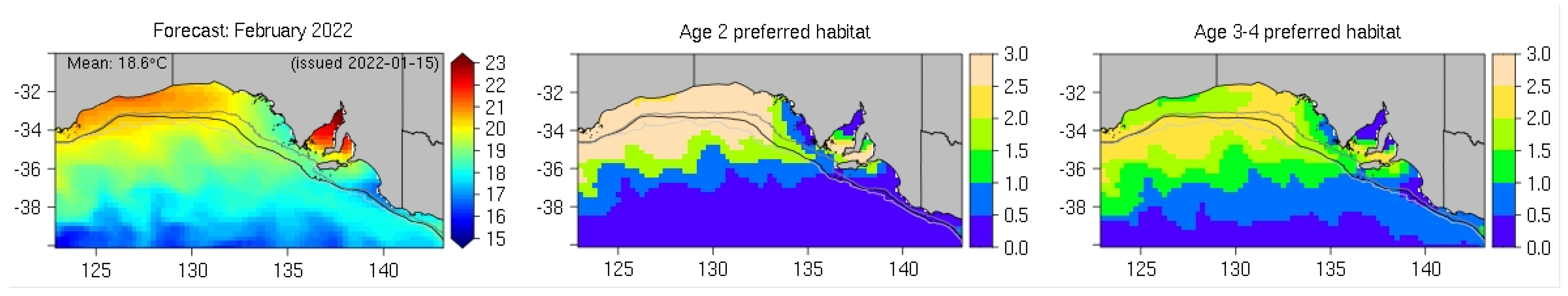
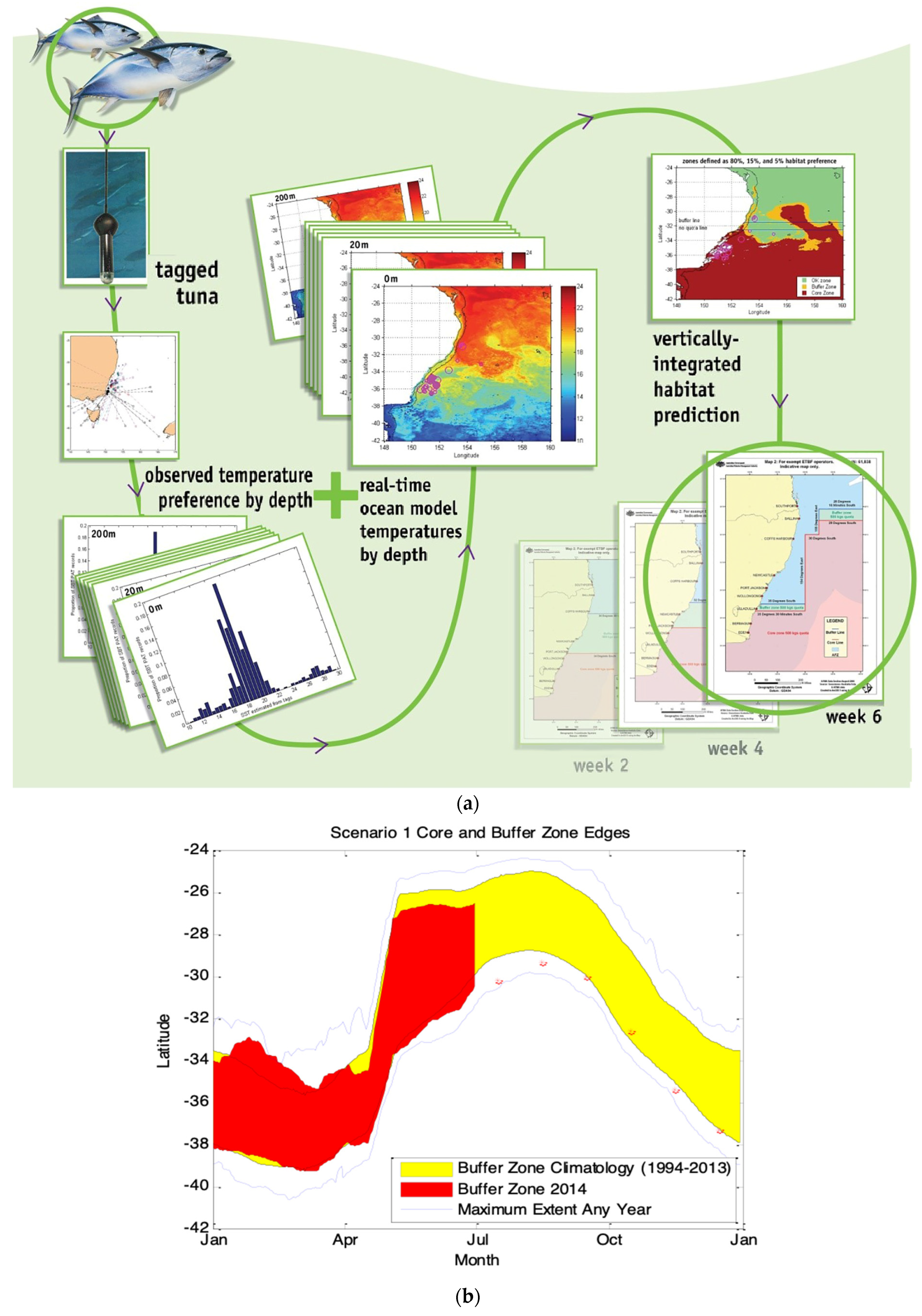
2.1.1. Case Study 1—Southern Bluefin Tuna in the Great Australia Bight

Large numbers of juvenile southern bluefin tuna (SBT) (Thunnus maccoyii) are found in the Great Australian Bight (GAB) during the austral summer (Dec-Apr). Here, they are caught in a purse-seine fishery worth ~AUD 41 million annually (2019-20 value) and towed in pontoons back to Port Lincoln (~135° E 35° S) to be grown and fattened before harvest several months later. There have been changes in the distribution of SBT in the GAB over the past decade, with fish being distributed further east than previously observed and the majority of purse-seine catches no longer occurring in traditional fishing areas. The presence of fish in unusual locations makes fishing operations for stocking the ranching pontoons challenging because the slow pontoon towing speed precludes a rapid response to shifts in fish distribution, so vessels need to be positioned prior to fish arrival.

In 2012, the Australian Southern Bluefin Tuna Industry Association recognized the need for scientific support to improve operational planning. They funded a project to provide seasonal forecasts (1 week to 2 months in advance) of areas of preferred SBT habitat. Environmental variables influencing the spatial distribution of SBT in the GAB during summer were examined using location data collected from electronic tags on SBT over many years, and ocean conditions where fish were found were compared with conditions available throughout the region and time period of interest [37,38]. Sea surface temperature (SST) was found to have the greatest influence on fish distribution, with fish preferring waters of 19–22 °C. Once habitat preferences were established, this information was coupled with a seasonal climate forecasting system developed by the Bureau of Meteorology (POAMA: Predictive Ocean Atmosphere Model for Australia) to predict locations of preferred SBT habitat in future [38,39]. A website, updated daily, was created to provide the industry with forecasts of environmental conditions and SBT distributions up to two months into the future, along with a suite of other relevant information, including forecast skill (www.cmar.csiro.au/gab-forecasts (accessed on 1 December 2022)). As the SBT fishery is quota-managed, the forecasting system was not designed to increase catches (and thus impact sustainability) but to enable fishers to better plan their operations and potentially increase efficiency and profitability.

In 2020, POAMA was decommissioned by the BoM and superseded by a new state-of-the-art seasonal climate forecasting model referred to as the Australian Community Climate Earth-System Simulator–Seasonal (ACCESS-S). One of the key benefits of ACCESS-S is the increased spatial resolution of the ocean model, from approximately 200 km longitude × 100 km latitude with POAMA, to 25 km × 25 km with ACCESS-S. To keep the forecast delivery website operational, a follow-up project updated the forecasting system to use ACCESS-S. Although the decommissioning of POAMA was the initial motivator for the follow-up project, another important factor was the availability of additional electronic tag data. These new data allowed for verification that the habitat models were still relevant, and enabled age-specific preference models to be developed. The age-specific models showed that fish ages 3–4 (the ages of most interest to industry for ranching operations) prefer slightly cooler surface temperatures (18.5–21.5 °C) than fish ages 2 (19–22 °C), which can make a noticeable difference to the areas deemed to contain the preferred habitat (Figure 2).

Based on feedback from industry members and an industry liaison representative, the website has been used consistently in the lead up to and throughout every fishing season since its development and has proven a valuable tool for fishers making decisions concerning when and where to position vessels and conduct fishing operations; for instance, in the 2017 and 2019 fishing seasons, forecasts indicated slow and delayed warming of the GAB so companies opted to delay fishing operations rather than send boats, pontoons, and crew out to sit idle for weeks until conditions became suitable for SBT [39,40].

The current habitat preference models are estimated using data obtained from electronic tags deployed on SBT mainly during 1998–2011, from only six tags from 2015–2017. Thus, it has not been possible to evaluate whether preferences have changed over the past two decades, which is particularly important given warming waters and other oceanographic changes in the GAB under climate change. To ensure that the habitat preference forecasts continue to be relevant, more recent biological data, ideally from further electronic tagging, must be obtained (noting that this is a large undertaking and funding would need to be established). Furthermore, environmental variables other than SST also influence the distribution of SBT in the GAB (e.g., subsurface temperature, chlorophyll, salinity). These variables are not currently available as forecasts, so they are not included in the habitat forecasting models; however, this is an area worth pursuing as more forecasted variables become available in future.

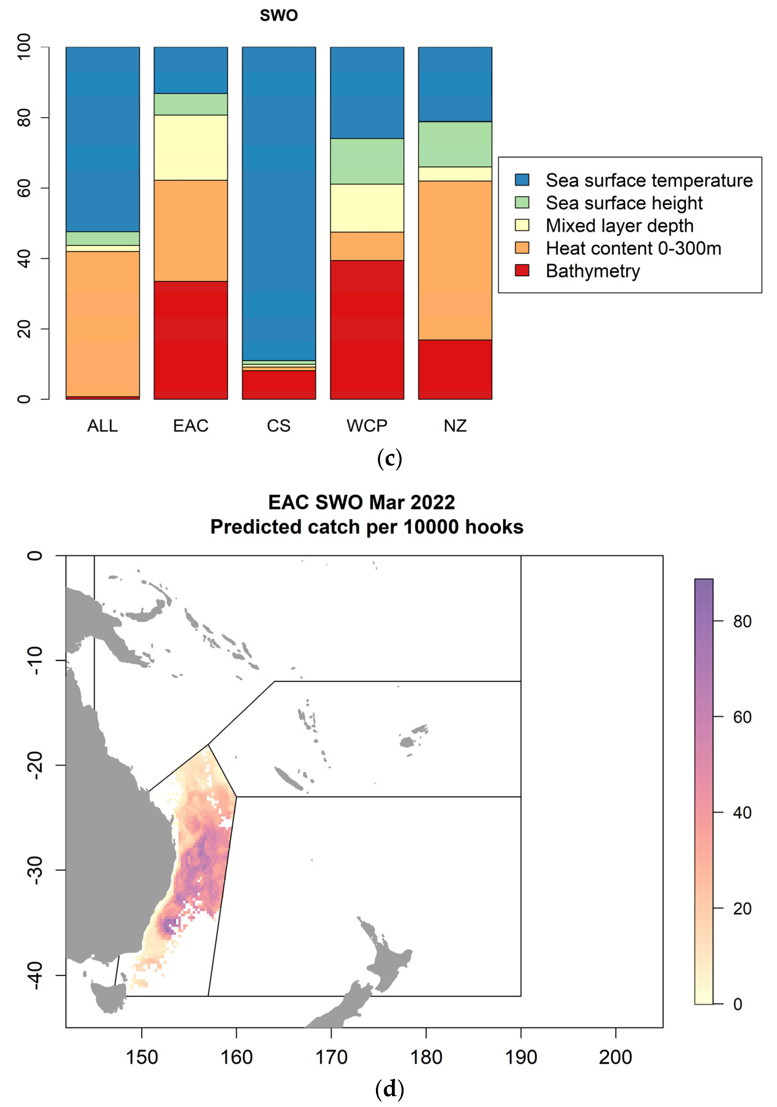
2.1.2. Case Study 2—Forecasts in a Multispecies Longline Fishery in Eastern Australia

The Australian Eastern Tuna and Billfish Fishery operates along much of the east coast inside and beyond the exclusive economic zone (EEZ) with effort concentrated in the dynamic portion of the East Australian Current. This multispecies longline fishery is managed by integrating single species assessments, catch limit trigger points, harvest strategies, and gear restrictions in a whole-of-area management approach. Historically, the five main target species in the fishery have been Bigeye Tuna, Thunnus obesus; Yellowfin Tuna, Thunnus albacares; Albacore, Thunnus alalunga; Striped Marlin, Kajikia audax; and Broadbill Swordfish, Xiphias gladius, but more recently, fishers have also been targeting Southern Bluefin Tuna (SBT, Thunnus maccoyii), an internationally quota-managed species.

Regular fortnightly reports were provided from 2003 onwards to the Australian Fisheries Management Authority during the fishing season [41]. These reports presented a habitat preference model providing near-real-time advice to management about likely SBT habitat. Managers used these habitat preference reports to frequently update spatial restrictions to fishing grounds. These restrictions, which were enforced by vessel monitoring systems and fisheries observers, limited unwanted interactions by fishers that did not hold a SBT quota (SBT cannot be landed without a quota, and in that situation must be discarded), and allowed those with a SBT quota to operate efficiently [41].

The habitat prediction system integrated tagging data from SBT, near real-time sea surface and sub-surface temperatures from a three-dimensional ocean model, and output from the seasonal forecast POAMA model to provide a habitat nowcast and forecasts for 6 months (Figure 3a,b). This system was in operational use by the Australian Fisheries Management Authority since 2003, evolving over the years from a surface-only model to an integrated sub-surface model with seasonal forecasting capability to aid managers and fishers in planning for future changes in the location of the habitat zones [23]. Incorporating the seasonal forecasting component was an important step in informing and encouraging managers and fishers to consider decisions on longer timescales [23]. The delivery of this prediction system ceased in 2014 when the management system changed and no longer relied on a forecast of habitat distribution.

More recently, the influence of oceanographic conditions on species distribution for all key target species has been investigated. Boosted regression trees (BRTs) were used to identify oceanographic variables that best explain the observed patterns in catches in the region and other regions of the southwest Pacific (Figure 3c); full details of the modelling work can be found in [42]. Forecasted oceanographic variables could then be input to the BRTs to provide spatial forecasts of catch rates in future months (Figure 3d). This information can be used by fishers and managers in understanding likely abundance patterns in the short term. By considering a range of oceanographic predictors that reflect the subsurface ocean structure, this method has improved forecast performance over earlier approaches using surface only information.

2.2. Ecological Forecasts in Aquaculture

Aquaculture is the fastest growing food producing sector in the world, increasing 16-fold between 1985 and 2018 [43], and it is expected to accelerate further in the near future to meet global protein demand. However, it must overcome a range of challenges that threaten its operations, including managing its environmental impacts for sustainable coastal development. Major environmental impacts of concentrated finfish farming on surrounding waters include increased organic matter from animal feeding and waste, which can then lead to deoxygenated water, harmful algal blooms (HABs), and outbreaks of parasitic, bacterial, and viral diseases, resulting in major economic losses and livelihood hardships [44]. The industry is also vulnerable to climate change, which might cause HABs to occur more often and more intensely, compromise infrastructure, and change the habitat suitability for some aquaculture species. Consequently, both industry and regulators are looking to system-based decision support tools to assist operational sustainability. Increasingly, operational information systems that can provide environmental forecasts and risk assessments on conditions that may pose a threat to the industry are being developed and relied on to ensure aquaculture does not breach regulatory conditions and guide day-to-day operations at the farm level [45].

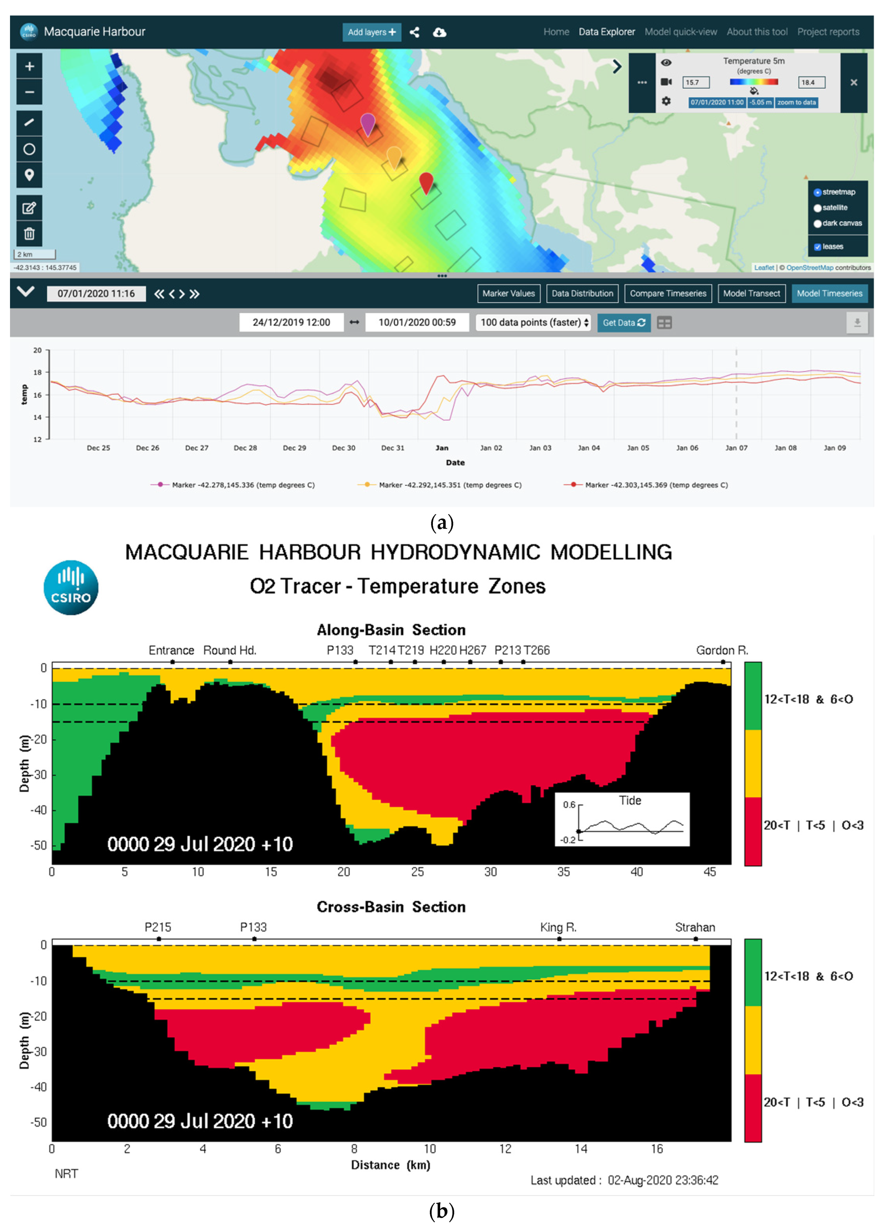
2.2.1. Case Study 1—Dissolved Oxygen Forecasts in Tasmania

The deep (50 m) and sheltered waters of Macquarie Harbour on the west coast of Tasmania support an economically important salmonoid farming industry. In recent years, however, episodic depletion of dissolved oxygen has contributed to major fish kills [46].

A three-dimensional hydrodynamic and biogeochemical model of the estuarine system was implemented to characterise the complex circulation and consequent variable oxygen concentrations in the harbour [47]. The harbour is 35 km long and 8 km wide, with a narrow ocean channel to the northwest and freshwater input from two major river systems (Gordon–Franklin, King–Queen; combined catchment area 6900 km²). Tracer studies found that residence time in the harbour was longest in midwater (110 days) and low oxygen concentrations were persistent in this layer. Simulations showed that during periods of low river flow, marine intrusions crossed the shallow sill (5 m depth) at the harbour entrance and increased oxygen concentrations at depth; during periods of strong north westerly winds, low oxygen content in midwaters could be displaced upwards by marine intrusions into the aquaculture zone.

The model was assessed against observations of sea level, temperature, salinity, and dissolved oxygen from multiple sites throughout the harbour. Statistical evaluation confirmed that the model adequately simulated the near real-time variation in dissolved oxygen concentrations in the harbour, based on observations from an operational profiling mooring.

Results from the hindcast, near real-time, and short-term forecasting model were provided on a dashboard, with visualisation tools that enable interactive selection and display of model output (e.g., timeseries of oxygen saturation at three locations, Figure 4a), together with the latest observations of water quality from the automated profiling mooring. The information dashboard was available to fish farmers and included a simple water quality index to show favourable and unfavourable temperature and oxygen conditions for salmonoids along a transect through the harbour (Figure 4b). The model information displayed on the dashboard supported tactical operational decisions, including the timing of smolt movements, stock harvesting, and the deployment of supplementary oxygen systems. As a result of this, the number of fish kills in the harbour were reduced.

In addition to tactical decision support, a number of multi-year scenario simulations were completed to explore long-term drivers of low oxygen in the harbour. Scenarios showed that under reduced river flow and/or reduced anthropogenic loads, oxygen conditions were predicted to improve throughout the harbour. These findings provided evidence to underpin the Environment Protection Authority’s strategic decision to limit the biomass of salmon in farms in Macquarie Harbour. At the time of writing, oxygen conditions throughout the harbour were slowly improving.

The modelling system deployed in Macquarie Harbour provided water quality forecasts to support strategic planning and tactical operational decisions for salmon aquaculture. Circulation in the harbour is strongly modulated by river flow which was estimated from rainfall scaled against a historical timeseries of river flow data. A useful improvement to the study would be to include a catchment model, including episodic dam discharge, for more reliable prediction of river flow. A further development to the system could provide extended forecasts at seasonal timescales and for future climate change scenarios, inform long-term planning of salmon industry operations.

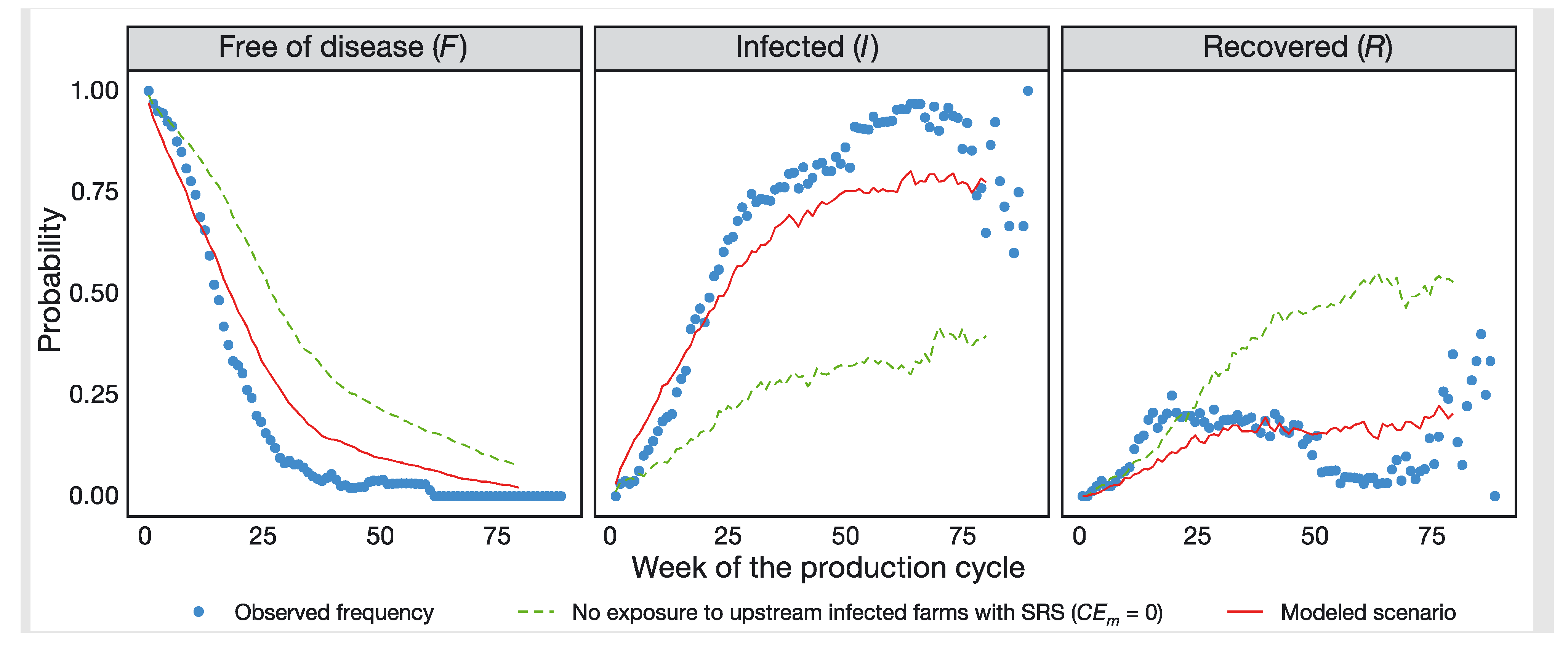
2.2.2. Case Study 2—An Operational Information System for Managing the Chilean Aquaculture Industry

The Chilean aquaculture industry in Patagonia, an area of ∼ 300,000 km², has been challenged by recurrent disease outbreaks and harmful algal blooms, which have caused substantial economic losses for the industry and erosion of social license to operate [48]. To address the sustainability and competitiveness of the Chilean aquaculture industry, the SIMA (Spanish for Integrated Management System for Aquaculture) Austral information system was commissioned by the Chilean government in 2015 and has been operational since 2019 [30].

SIMA is a comprehensive decision support tool developed for the Chilean Aquaculture industry and government agencies to provide access to improved environmental intelligence. SIMA integrates available historical and near-real time observation data and physical and socioecological models to create decision support tools (Figure 1). Users can generate regulatory and non-regulatory reports through a web-based dashboard, and access tools for strategic and tactical planning and incident response (such as disease outbreaks). The information underpinning SIMA is derived from routine (daily to weekly) production and environmental data and near real-time output from regional-scale environmental and socioecological models. The coupled environmental models (hydrodynamic, biogeochemical, sediment, and stream flow) predict environmental conditions such as oxygen concentration and temperature to assess the suitability for production. They also provide warnings for mitigation if environmental properties might cause a negative impact, so that the industry could alter operational behaviours if necessary, such as changing feeding patterns or harvesting early. Maps and time series for major indicators (such as aquaculture production, biomasses, fish catch, disease levels, income, and revenue, etc) are produced by the regional-scale socioecological models (linking more than 20 other statistical, process, and agent-based approaches). This information is delivered directly as data layers within a hierarchical Ecological Risk Assessment framework. Individual models can use data from other parts of SIMA to answer a particular question (e.g., an epidemiological or economic question) or they can form a systems model for the entire region to inform strategic responses under different market, management, or environmental scenarios identified by users [49]. The farm-scale epidemiological and economic models offer tactical support for farm operators. The epidemiological model is a statistical probabilistic model with its parameters and transition probabilities between infection states estimated on a regional scale from the weekly data reported by industry. The model simulates fish growth, and forecasts mortality and disease dynamics for three finfish species (Atlantic salmon Salmo salar, Coho salmon Oncorhyncus kisutch, and rainbow trout Oncorhyncus mykiss) and two common diseases, Salmonid Rickettsia Septicemia and bacterial kidney disease. Fish growth, survival, total production, and disease prevalence are predicted by the model. The economic model is coupled with the epidemiological model to provide cost and revenue estimates based on operation behaviours of the farms.

Several SIMA models can work together to evaluate disease transmission and risk mitigation. The Environmental Model climatology, together with a connectivity tool (CONNIE), can be used to investigate the transmission between farm locations and execute incident response in near real-time. This can be used by a range of practical applications, including assessing the risks of pathogen exchange between leases such as the predicted probability of Piscirickettsiosis disease as a function of the week of the salmon farming cycle for the SIMA Chile system validated by observations (Figure 5). Results from these models demonstrate that hydrodynamic connectivity between farms plays a major role in disease prevalence and waterborne transmission of the disease [50].

2.3. Ecological Forecasts of Harmful Algal Blooms

HABs can cause direct and indirect negative impacts to aquatic ecosystems, coastal resources, aquaculture (see Section 2.2), and human health (through consumption of contaminated drinking water or shellfish) [51,52]. Ecological forecasts of HABs have been developed around the world, recognising their threats to public health, ecosystem health, aquaculture, tourism, and other blue economy industries [53,54]. However, there are major challenges in the operational forecasting of HABs. The efficacy of the forecasting relies on location-specific HAB species and local oceanographic conditions and may need a range of data types such as satellite remote sensing data, field observations (e.g., samples and glider data), and oceanographic and meteorological monitoring data from buoys or surface temperature/current data, as well as a range of models and forecasts such as wind forecasts or transport models.

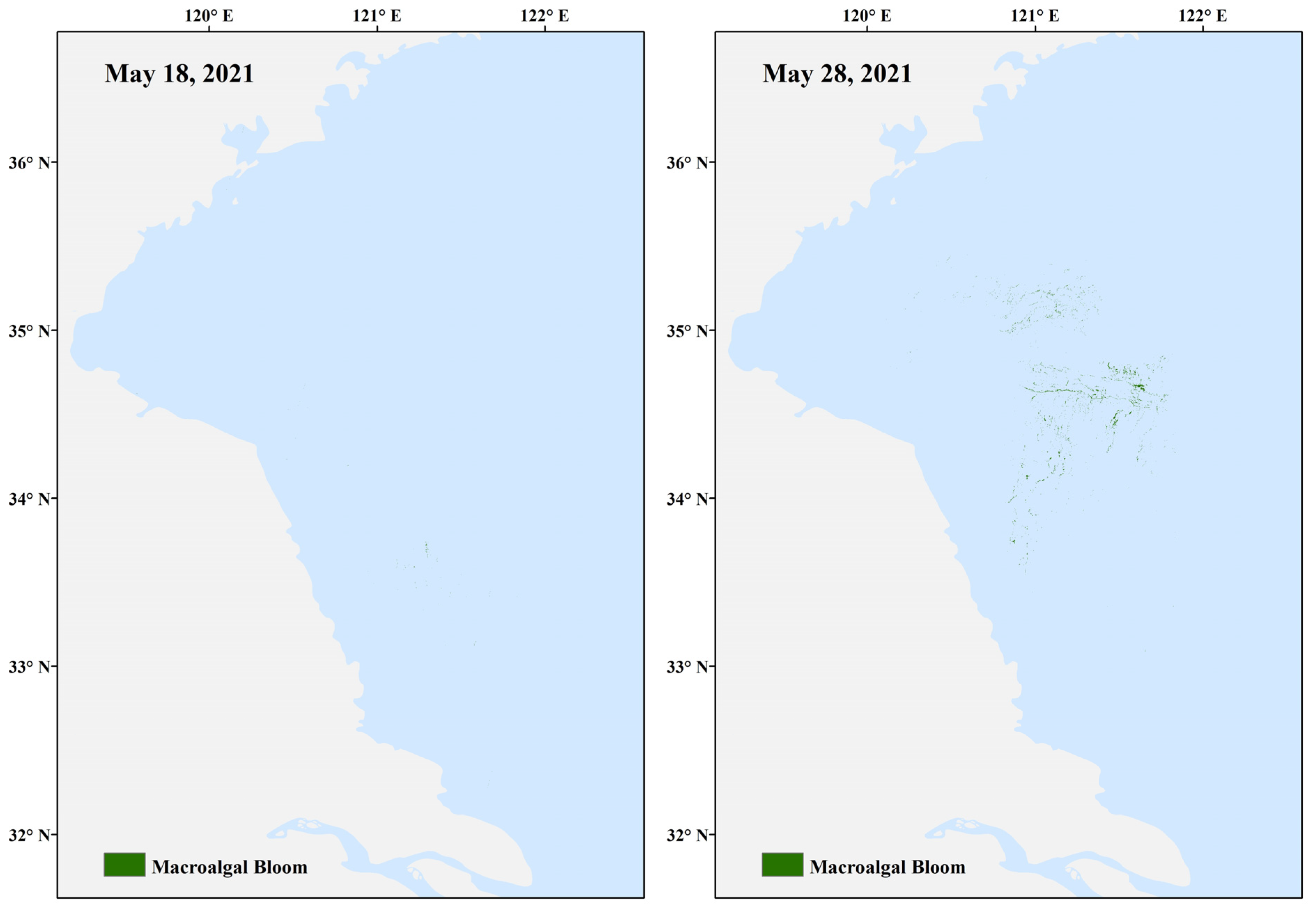
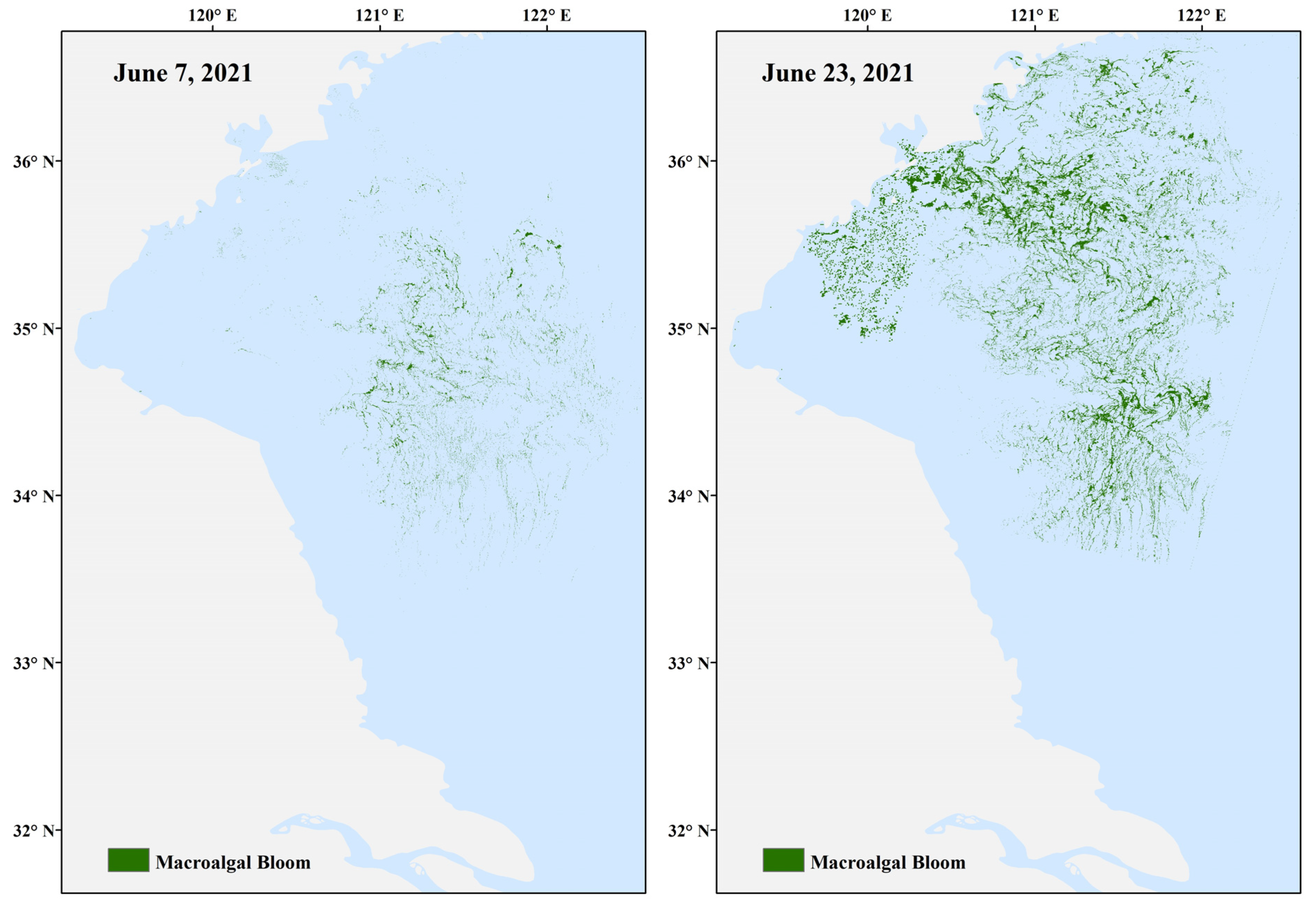
2.3.1. Case Study 1—Real-Time Forecasting of Harmful Algal Blooms in the Yellow SEA

Since 2007, macroalgal blooms of Ulva prolifera, known as “green tides”, reach Qingdao (China) beaches each year. During the 2008 Beijing Olympics, the sailing event was affected and the government mobilised millions of people to clean the beaches. The tourism industry suffered as the blooms usually reach Qingdao in July-August, the peak tourism season. Central and regional governments have implemented a series of mitigation measures, targeting the source region of green tide to prevent its expansion and formation into an intense green tide, as well as interception at sea before it reaches Qingdao beaches. There is considerable interest in monitoring and forecasting methods to aid interception, collection, processing, and utilization of green algae.

By using satellite remote sensing data to identify floating macroalgal blooms, a data-assimilating ocean general circulation model for the Yellow Sea successfully predicted the observed drift trajectory of floating macroalgae with a lead time of 6.5 days [55,56,57]. By calculating the Normalized difference vegetation index (NDVI) index from MODIS and Sentinel-2, an input dataset for the dispersing algae at a resolution of 1 km was created (Figure 6). The macroalgal blooms were treated as passive floating particles passively advected by the ocean currents. The drift trajectory of the blooms was predicted by the integration of modelled currents by the ROMS (Regional Ocean Model System) model for the Yellow Sea. The ROMS model provides a 6.5-day forecast, initialised by assimilating sea surface temperature, sea surface height, Argo observations, and real-time observation of salinity and temperature data from Yellow Sea stations. By coupling the growth process of floating algae, the forecasting model for floating macroalgae trajectories can be improved to further support the monitoring and prediction of macroalgal blooms adjacent to coastal cities. To improve future forecasts, the relationships of macroalgal blooms with aquaculture rafts, water temperature, salinity, and other environmental factors in the Yellow Sea need to be further explored and incorporated, and remote sensing algorithms for detecting the blooms needs to be further improved.

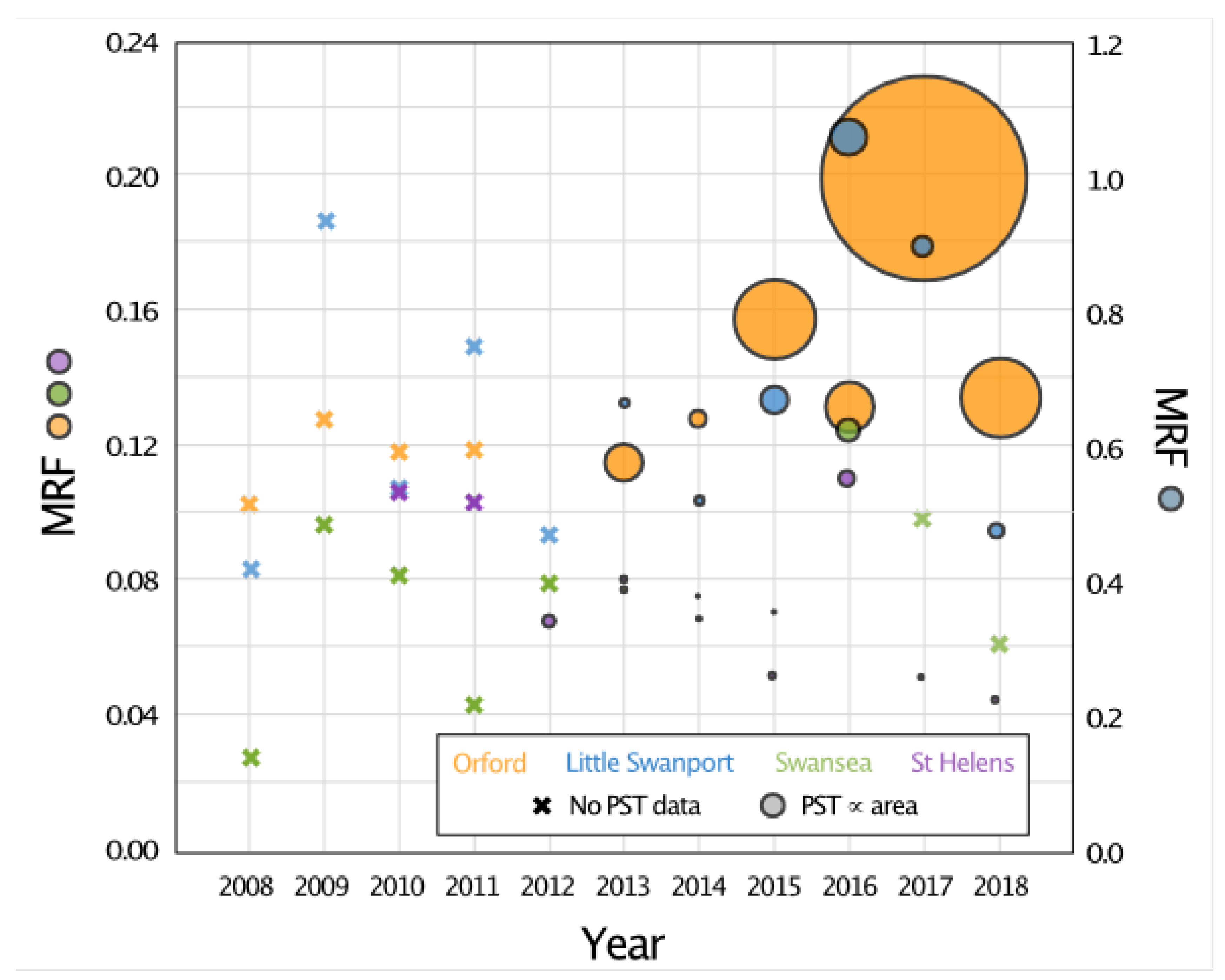
2.3.2. Case Study 2—Toxic Algal Blooms in Tasmanian Coastal Waters

In many parts of the world, dinoflagellate species from the genus Alexandrium form HABs by producing paralytic shellfish toxins [58]. Since 2012, Alexandrium catenella has been detected in coastal waters off eastern Tasmania from June to October, where they have been responsible for life-threatening instances of human paralytic shellfish poisoning, as well as extended closures of fisheries and aquaculture for mussels, oysters, abalone, and rock lobster [59,60]. Although there is a need to detect and forecast A. catenella blooms because they are toxic, their low biomass provides major challenges for traditional detection approaches such as satellite remote sensing. Development of a forecasting capability has therefore focused on identifying relationships of blooms to local meteorological, hydrological, and oceanographic conditions.

Statistical analyses have shown that A. catenella blooms off eastern Tasmania are often associated with the transition from persistent upwelling favourable winds (southward) to weak or downwelling favourable winds (northward), with accompanying changes in sea surface temperature and chlorophyll [61]. Relaxation of upwelling winds allows warmer offshore water to move towards the coast, where it can enhance local stratification. Because dinoflagellates are mostly positively buoyant, they tend to be carried onshore and are concentrated in the upper water column [62], where they are most likely to influence aquaculture and coastal fisheries. An understanding of these mechanisms can be used as a basis for ecological forecasting. For example, environmental factors that enhance coastal stratification have been combined within a single meteorological risk factor defining the energy balance between the influence of air temperature and/or rainfall in increasing stratification, and wind-driven ocean mixing in eroding stratification [59]. Over the short history of A. catenella blooms off eastern Tasmania, there has generally been an upward trend in the meteorological risk factor, with corresponding increases in observed paralytic shellfish toxin levels (Figure 7).

Although routine ecological forecasting for A. catenella in eastern Tasmania is yet to be realised, improved understanding of the underlying physical drivers provides a foundation for a system based on standard meteorological data. Alternatively, given that meteorological drivers were originally chosen as proxies for stratification and onshore flow, operational oceanographic models able to resolve the key coastal processes may ultimately provide more direct and reliable predictions.

2.4. Ecological Forecasting for Risks to Iconic Habitats or Their Users

Growing coastal populations and increasing coastal development, along with climate change, is leading to increased pressure on iconic coastal habitats, e.g., [5]. Threats can be to the habitats directly, such as with marine heatwaves leading to coral death (Case Study 1 Coral bleaching), via biological interactions with the habitats (e.g., Case Study 2 Crown-of-thorns starfish), or to humans making use of iconic habitats via tourism (Case Study 3 Irukandji jellyfish).

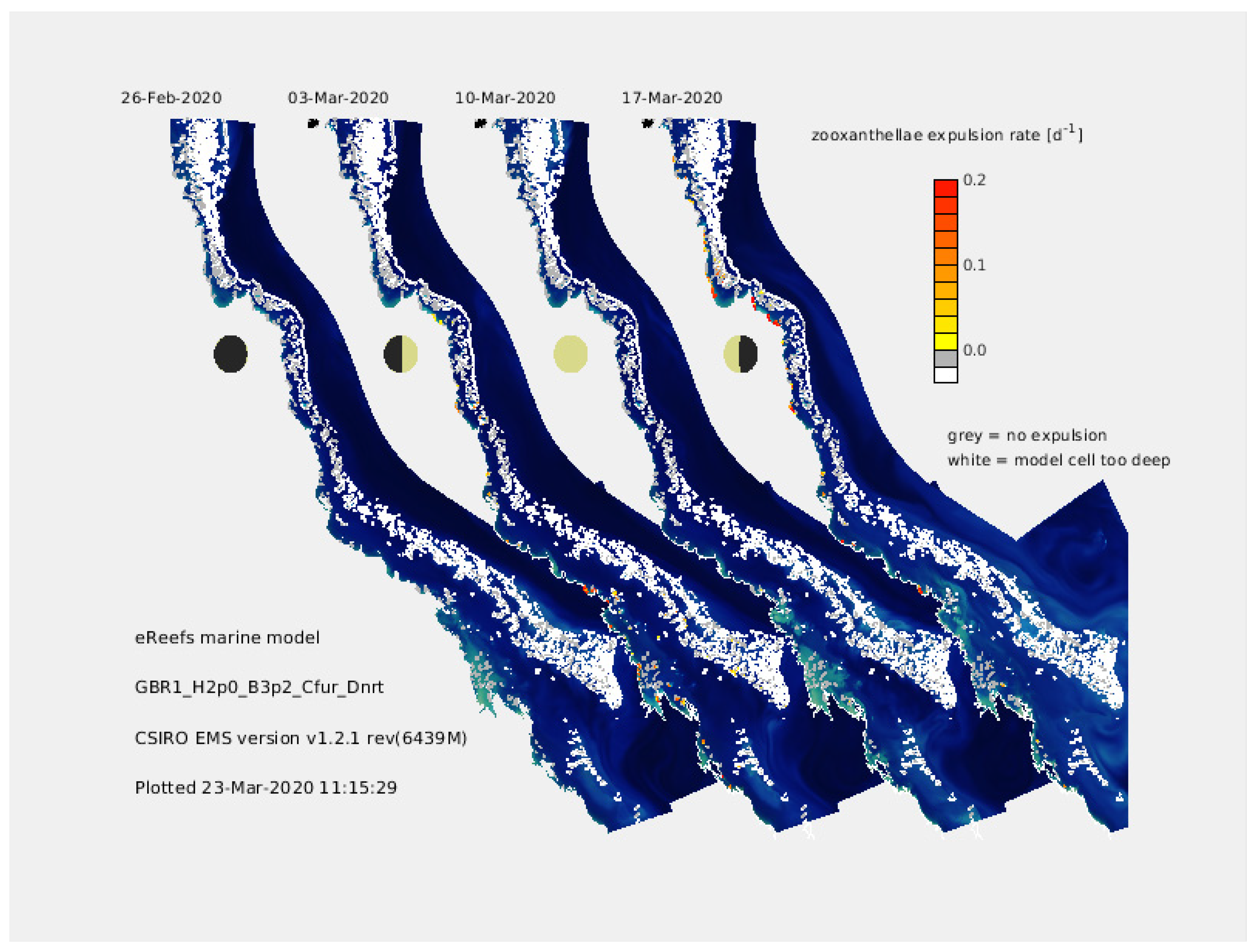
2.4.1. Case Study 1—Near Real-Time Forecasts of Coral Bleaching on the Great Barrier Reef

Mass coral bleaching driven by ocean warming has emerged in the 21st century as the greatest threat to the health of the coral reefs globally [63]. In recent times, the Great Barrier Reef (GBR) has suffered widespread bleaching events in 2016, 2017, 2020, and 2022. Aerial surveys can observe surface bleaching rates along flight paths, but processed data takes months to be available and is not spatially complete.

The eReefs Project [31] has developed a 1-km resolution coupled hydrodynamic-biogeochemical model that has been run in near-real time since 2016. The biogeochemical processes include a mechanistic model of the coral-symbiont relationship that considers temperature-mediated build-up of reactive oxygen species due to excess light, leading to zooxanthellae expulsion. The model explicitly represents the coral host biomass, as well as zooxanthellae biomass, intracellular pigment concentration, nutrient status, the state of reaction centres, and the xanthophyll cycle, and the internal concentrations of reactive oxygen that leads to bleaching [64]. A hindcast of the model for 2016 showed good correspondence between processed aerial survey data and model zooxanthellae reactive oxygen concentrations (Figure 8, [64]).

The latest version of the near-real time biogeochemical model, including the coral bleaching submodule described above, has been run since 16 October 2019 [65,66], capturing the 2020 GBR bleaching event that was considered widespread but mild. The simulation is archived in near real time on the publicly-accessible National Computing Infrastructure (see eReefs Research (csiro.au) for details). The simulation is maintained at between 4 and 6 days behind the present, a result of waiting for ocean and atmospheric forcing products and the ~1 real day duration to run 3 days of simulation time.

The simulation shows that during some periods, there was sufficiently high thermal stress on some reefs, combined with elevated bottom light levels, for the reactive oxygen stress to become toxic and to begin zooxanthellae expulsion, or bleaching (yellow to red pixels, northern GBR, Figure 8). The levels do not appear to be as high as in 2016 or 2017 [66]. The distribution of bleaching-level stress is restricted to the inshore and mid-shelf regions. The greatest rate of zooxanthellae expulsion (up to 0.3 d-1, enough to pale a coral skeleton in a few days) was found on inshore reefs between Cooktown and Princess Charlotte Bay on the 17 March 2020 during neap tides of the 3rd quarter moon (Figure 8). Around this time, seabed temperatures reach their maximum for the summer. Neap tides correspond to low current speeds, and less resuspension, resulting in greater light levels on the seabed. Furthermore, the few days preceding the 17 March had low cloud cover. Thus, 17 March had the most intense bleaching conditions for 2020.

In addition to these simulations in hindcast mode, forecasts at a 3-day lead time have been produced, although they are not yet routinely used. The nowcast is part of an internally maintained information system and the results are currently provided through emails to stakeholders. A summary of the seasonal outlook is provided by written reports.

At present, management options for preventing coral bleaching are limited. Thus, the present value of forecasts of bleaching from a numerical model are simply in their spatial coverage and the quantification of bleaching in hard-to-observe deeper waters. In the future, management intervention may be deployed to reduce bleaching through solar radiation reduction and/or introducing temperature tolerant corals [67]. The optimisation of these deployments, especially solar radiation reduction, will require spatially-resolved forecasts of bleaching.

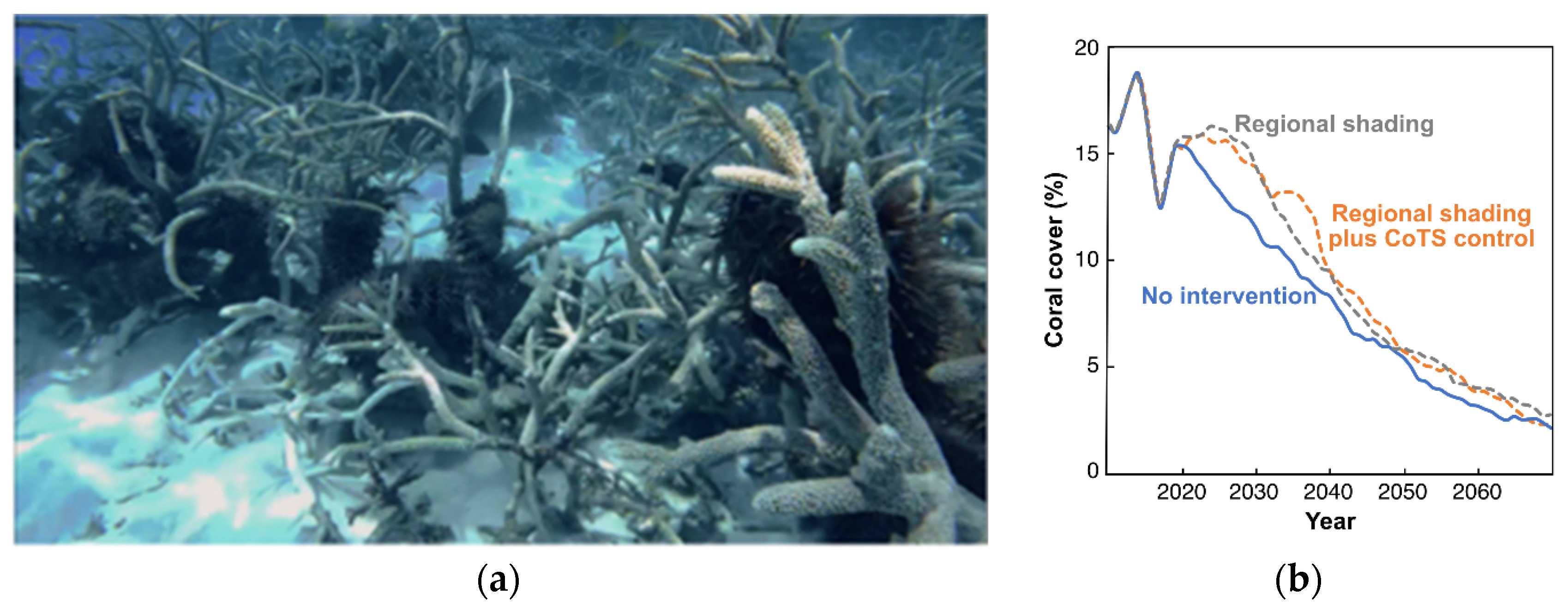
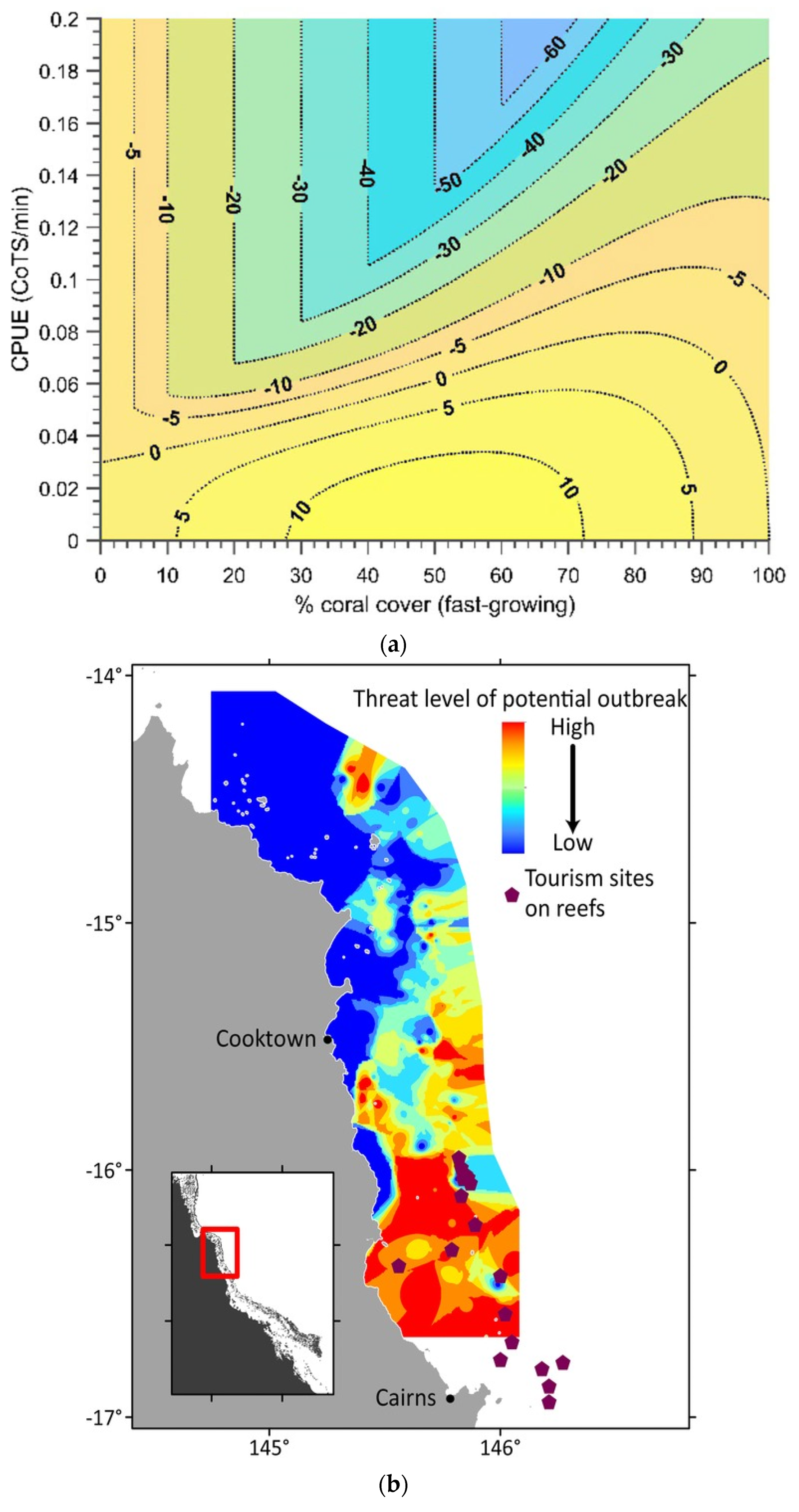
2.4.2. Case Study 2—Forecasting to Inform Suppression of Crown-of-Thorns Starfish on the Great Barrier Reef

Coral reefs have long faced a wide range of threats, including diminishing water quality, overfishing, and coastal development [63] However, processes related to climate change, in particular warming and its impacts on coral bleaching, are increasingly threatening coral reefs [68], especially on the Great Barrier Reef [63,69]. Other major causes of coral mortality include cyclone damage and predation by crown-of-thorns starfish [70]. Outbreaks of crown-of-thorns starfish (Acanthaster cf. solaris, hereafter COTS) on the GBR are one of the main causes of the ongoing coral decline in that location [70,71,72], and cause coral decline throughout the Indo Pacific [69,73]. The GBR is now experiencing its fourth starfish outbreak since the 1960s, and mortality due to COTS is likely to continue to be one of the largest contributors to coral decline on the GBR. Given that it will be decades before global warming is halted or reversed, reducing predation on corals by direct action to cull COTS is the most effective means to prevent loss of coral cover over short time scales [74].

COTS control on the GBR is now part of the management policy for the entire reef. This was not always the case, since management authorities considered the benefits of large-scale control would not justify the costs of implementation [75]. This change is due not only to the changing urgency of the need to preserve corals, but also to the higher levels of confidence among reef policy makers around the effectiveness of COTS control, its likelihood of success, and the costs of inaction. Modelling shows that controlling COTS results in much better outcomes for the GBR in terms of its overall coral cover than if other management strategies were implemented with no attempt at active control (Figure 9, [67]).

Among the reasons for the success of recent control efforts on the GBR relative to previous attempts is the adoption of Integrated Pest Management principles [74]. The application of these principles to COTS on the GBR has relied heavily on several ecological modelling approaches. To allow effective COTS density targets to be determined, control target thresholds relevant to maintaining coral cover have been determined through MICE (Models of Intermediate Complexity for Ecosystems) models combining multiple coral types and multiple COTS life history stages (Figure 10a, [76]). Another important component of the Integrated Pest Management approach in a system of over 2000 individual reefs is the ability to prioritize reefs for control, in part based on their connectivity with other reefs and the network dynamics of the system. Using hydrodynamic particle dispersal models and network analysis (Figure 10b, [77]), reefs most important as sources of COTS larvae to the rest of the GBR system can be targeted for control. Modelling of the COTS phenomenon at the GBR scale also showed an inherent cyclicity in COTS outbreaks, allowing the timing and location of a likely fifth outbreak to be predicted [78]. This has allowed for targeting of pre-outbreak COTS populations with a view to suppressing future outbreaks.

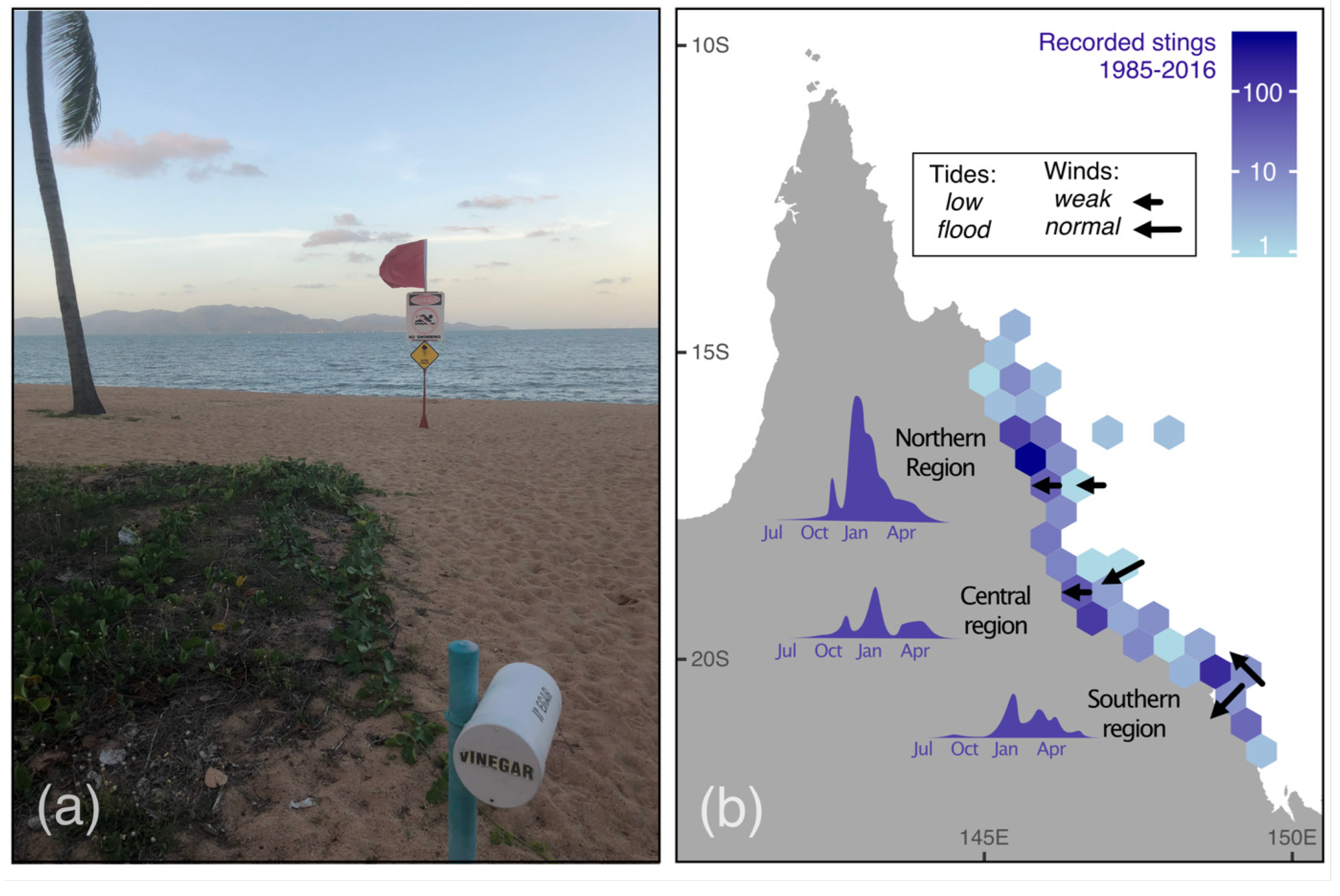
2.4.3. Case Study 3—Real-Time Forecasting to Manage Risks Posed by Irukandji Jellyfish on the Great Barrier Reef

Irukandji are small (about the size of a thumbnail) transparent jellyfish found in coastal tropical waters globally. Their stings produce debilitating illness and are potentially fatal [80,81]. Their presence imposes major financial costs on tourism and fisheries sectors [82]. With their small size, Irukandji cannot be easily monitored or excluded using physical barriers such as nets. Managing threats to swimmers and divers can be improved via prediction of their presence from local meteorological and oceanographic conditions to guide the closures of beaches and other marine operations (Figure 11).

De-identified records of Irukandji stings from hospitals and surf lifesaving clubs over nearly 30 years were combined with Irukandji sampling data from the Great Barrier Reef (GBR) region to support development of a forecast model based on a generalised linear model [83]. The number of Irukandji stings per day was the response variable [78] and several environmental variables were included as predictors. In addition to the well-established seasonality (December to April), wind direction was the most important predictor, with most areas having a higher incidence of stings during periods of weak, westerly or north-westerly winds (Figure 11b). Under these conditions, any jellyfish migrating upwards in the water column will tend to accumulate along the coast [84]. Incoming tides were also associated with more Irukandji stings on beaches in the northern and central GBR, the majority of which were around low tide or over the early phase of the flood tide.

Responding to operational forecasts of Irukandji sting risk requires a trade-off between reducing stings and closing beaches and marine tourism operations such as reef diving, with associated financial losses. For example, in the northern GBR, the percentage of sting days avoided through use of the model would be expected to be approximately 30% more than the percentage of closure days. For example, one intervention strategy (beach closure when southeasterly wind reverses to northwesterly wind) affected 31% of all days and reduced sting days by 61% [81]. This large effect highlights the efficacy of the forecast model (percentages would be equal if the operational model provided no benefit and closures were effectively random). There is significant potential for further improvement in the forecast model through harnessing detailed oceanographic data on coastal flows and predicted accumulation patterns from existing models such as the eReefs model [31]. Particle-tracking approaches have been used extensively in the GBR region to model the movement of a wide range of planktonic organisms [85,86,87] and could be used here to better understand oceanographic conditions prior to major sting events. For example, given we know sting locations and that the lifecycle of Irukandji is likely to be about 2 weeks [88], there is potential to use particle-tracking to trace back in time and space to find the currently unknown source populations of the benthic polyps. This approach might also afford a greater degree of understanding of oceanographic conditions such as temperature that might trigger strobilation by the benthic polyps leading to the pelagic Irukandji stage that we are familiar with. Although there is potential to deploy models to support operational prediction of Irukandji risk on the GBR, this has been prevented by the absence of an agency with both a mandate and sufficient capacity to operate a system delivering routine forecasts. For example, most Irukandji stings are off public beaches where bathers are not the responsibility of particular tourism operators, health authority responsibilities are limited to post-sting treatment, and volunteer lifesaving organisations have no capacity to run operational forecast systems. Efforts to date have therefore focused on the provision of guidelines to lifesavers, tourism operators and other sectors operating in the GBR marine environment based on statistical relationships. The organisation with the closest mandate and capacity to provide forecasts is probably the Australian Bureau of Meteorology.

2.5. Common Features amongst Case Studies

Although different modelling approaches were used, the case studies had some common features (

Table 1. Case study summary showing the model method, delivery of a nowcast, forecast lead time, use of an information system, and uptake by end users.

Case study and Location	Method	Nowcast	Forecast Lead Time	Delivery Mode	Part of an Information System	Uptake
Fisheries
Tuna—eastern Australia	Habitat preferences	Yes	0–3 months	Email	No	Yes
Tuna—southern Australia	Habitat preferences	Yes	0–3 months	Website	No	Yes
Aquaculture
Hypoxia—Tasmania	Coastal model	Yes	<10 days	Dashboard	Yes, with interactive data explorer	Yes, but not sustained
SIMA-Austral Chile	Integrated models	Yes	Days to months	Website	Yes	Yes
Algal blooms
Yellow Sea, China	Ocean model	Yes	6.5 days	Website	No	Yes, but not sustained
Tasmania	Environmental correlation	Yes	0–3 months	Not yet	No	No
Iconic habitats and their users
Coral bleaching—GBR	eReefs models (hydrodynamic and biogeochemistry)	Yes	3 days	Email and reports	Yes (nowcast)	Yes (through reports, papers)
Crown of Thorns—GBR	Combined hydrodynamic and ecosystem models	No	A few years	Reports and publications	No	No
Jellyfish—Queensland	GLM	Yes	<3 days	Publications	No	Only as guidelines

). These examples commonly combined sustained and innovative observations with a modelling approach. Eight of the nine case studies produced nowcasts, which might be expected if the model is developed based on historical relationships. In the case of the east Australia tuna model, a nowcast was the forerunner to the forecast, as it was developed ahead of any forecasting capability. The time scales of forecasts were mainly from a few days to seasonal, probably reflecting the predictability in the system. One forecast system (COTS) had a lead time of several years because past summer spawnings continued to contribute to current populations. The delivery mode varied from email to websites to interactive dashboards. They all had a value for decision making, however, not all the forecasts have been taken up by stakeholders, and of those that have been developed, not all were sustained.

3. Discussion

Although long-term prediction has been used to understand the future state of the ocean in response to climate change [12], near-term or seasonal environmental forecasts, which allow for rapid feedback for both model developers and forecast users, can lead to effective decisions for sustainable ocean use and management given the increase in pressure on the ocean [9]. Because ecological patterns in the ocean can impact human health, food, water, and the environment, ecoforecasting provides valuable tools to power the blue economy and build climate resilience for the coastal resource managers, private industry, and public. As the world’s environment is changing rapidly under climate change, ecoforecasting has been increasingly recognised as a national priority around the world [24,89]. However, there are significant challenges given the complexity of the ecosystems, the difficulty in modelling them, the lack of comprehensive observations, and considerable knowledge gaps. Nevertheless, significant progress has been made and the benefits of ecoforecasting to triple bottom line outcomes associated with ecosystem-based management has seen increased effort around the world in recent years.

3.1. Insights from the Case Studies

The case studies presented here span a range of forecast metrics (abundance, distribution, and phenology) applied to different species and predictions of various ecological events such as harmful algal blooms, starfish outbreaks, jellyfish blooms, and coral bleaching. Among the different forecast metrics, distribution was the most common [22]. Abundance continues to be a difficult ecological property to forecast, and traditional population models are yet to be routinely combined with environmental drivers. Most forecasts covered relatively short time periods from several days to several months, and all had a clearly identified management problem. They have allowed resource managers and other stakeholders to make decisions on how to respond to ecological events that may affect economies, communities, and environments.

3.1.1. A Clearly Identified Management Problem Benefits from Environmental Intelligence

Although the case studies presented here could all be considered successful as a skillful forecast was produced, the engagement between developers and end users varied substantially. In some cases, this may have limited the uptake (e.g., hypoxia forecast in Macquarie Harbour). In other cases, there were close interactions between the parties and the forecast that solved a management problem identified by end users with an operational information system explaining the results clearly and visually, and it was readily taken up by stakeholders (e.g., the SIMA-Austral information system on Chilean salmon farming; SBT in the Great Australian Bight).

3.1.2. Operational Information Systems can Enhance Forecast Value

Ecoforecasting can integrate a wide range of research, from observations to multiple models. However, they often require expertise and understanding of models to interpret the forecasts correctly. This requires extension efforts and end user education [38]. Delivery approaches varied, from simple to complex, depending on the end user.

An operational information system, which runs in real-time and provides easy-to-access information on environmental conditions and early warnings of potential harmful events, effectively translates a technical forecast into practical information, providing a useful decision-making tool for government regulators, private industry, and the public alike.

A challenge in developing an operational information system is that it often requires significant investment in cyber infrastructure and capabilities, in additional to an observing network and a modelling system. It also takes some time to be set up and becomes operational. Another challenge is its ongoing maintenance, as evidenced by some of the case studies having stopped their operational systems due to lack of funding after the projects have finished.

3.1.3. An Enduring Funding Model Is Needed to Sustain and Develop the Field

Developing ecoforecasts using research project funding is problematic for sustained use when a project concludes. Some of the case studies presented here were successful in terms of their forecast skill, but were not implemented or were halted after the research projects ended. Researchers cannot typically sustain ongoing operational forecasts, which require infrastructure and sufficient funding for running the system, monitoring, maintenance, and service distribution [NOAA’s process to make ecological forecasts operational]. As part of developing an operational forecast, developers should investigate how forecasts will meet user needs, if the user is prepared to use the product, and how it will be delivered when a project concludes [15]. For instance, the lack of an agency with both the mandate and the capability to deploy a forecasting system and maintain long-term delivery has been a limiting factor and prevented the uptake of the Irukandji forecast model in Australia.

National efforts could be one approach to sustained forecasting, as occurs with national weather prediction services. For example, Australia is building a National Environmental Prediction System, which could become the infrastructure backbone, although marine applications are rare in current discussions.

3.2. Gaps and Improvements

These marine examples from Australia, China, and Chile broaden the geographic scope reported in the review of ecological forecasting in [22]; however, this scan is not comprehensive and other examples elsewhere in the world will also be instructive. These selected examples are used to highlight some recent advances in the fast-growing field of ecological forecasting [22,28]. Connections between forecast teams, such as via the Ecological Forecasting Initiative (https://ecoforecast.org (accessed on 1 December 2022)), can help expand their use, although these initiatives and conference sessions tend to connect researchers from the Global North. One potential solution to make global connections may be the sharing of open-source code and development of transferrable and reproducible forecasts [16].

Ecoforecasts are iterative approaches [10], and thus present the opportunity for practice and feedback (similar to the weather forecasting community) by research teams and end users after each cycle of forecasting and delivery. Consideration of metrics for evaluating success (e.g., model accuracy threshold; [16]) can also focus a forecast team on continual improvement. Iterative processes to improve models acknowledge that imperfect models are sufficient as long as uncertainties and assumptions are presented clearly, and progress is made through a willingness to learn and improve. Improved data can also improve forecasts, such as additional data on the prey that also influences the distribution of the focal species (e.g., fisheries). These data are likely to be available from ecosystem models in future, but observational data are rare, and so inclusion of these predictors is difficult.

Co-development with end users can also result in additional improvement. Collaborative teams linking researchers and decision makers are needed to build the best approaches [16]. For example, visualisations such as infographics can help non-modellers understand the process and uncertainties in forecasts intuitively and incorporate measured risk during decision making [16].

Finally, the models we covered lack consideration of social ecological feedbacks, except the SIMA-Austral operational information system. Social factors can influence ecosystems and forecasts could also influence social systems [16]. Social-ecological drivers, interactions, and feedback can be directly built into the model, or social information could be used to interpret and contextualize the output of forecasts (e.g., [90,91]).

3.3. Recommendations

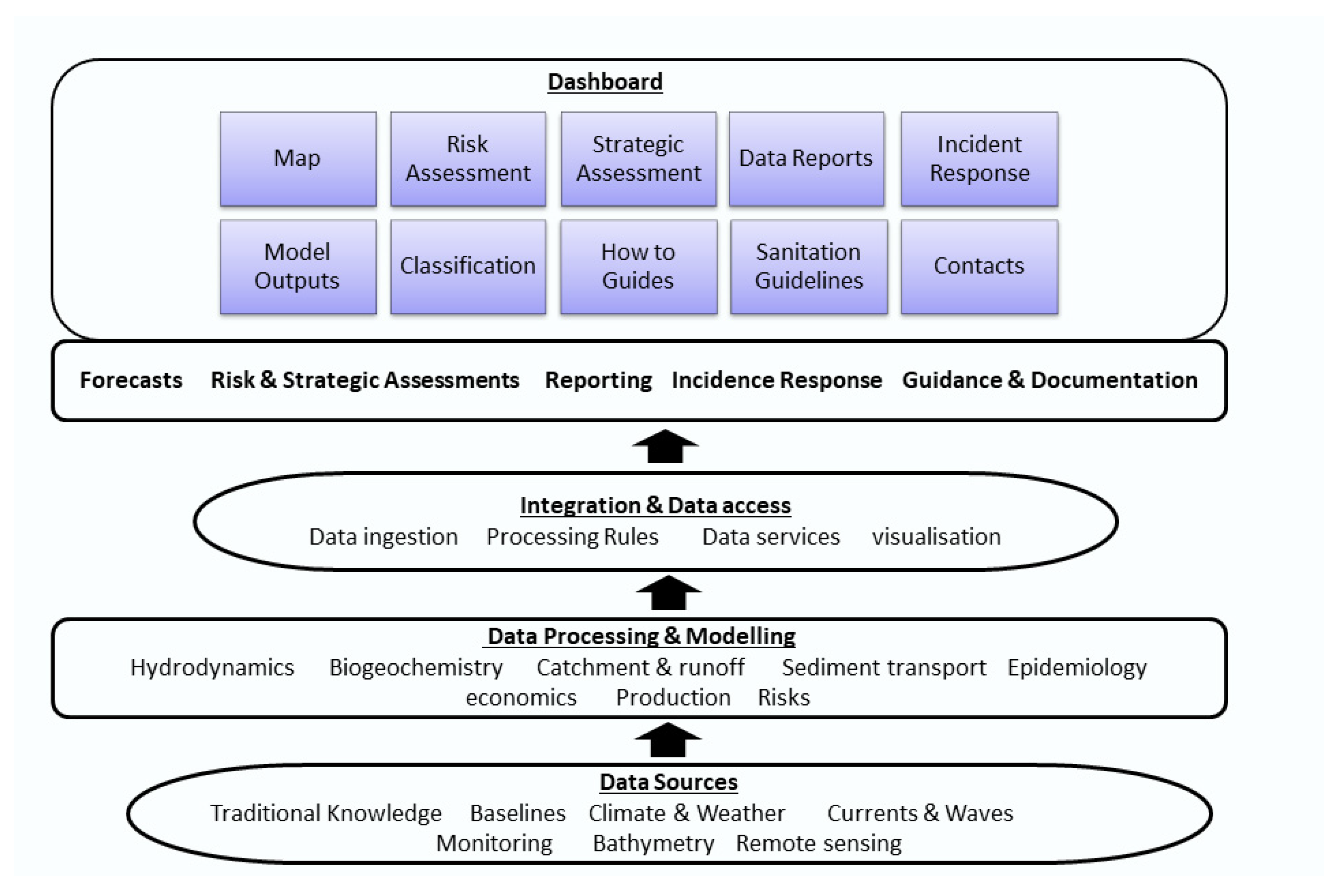
• Information systems can help end users. To integrate ecoforecasting into decision making, an operational information system that synthesises observations and modelling to provide easy-access information delivered through cyberinfrastructure can be used as a powerful tool to communicate a complex forecast. Not all forecasts need to be developed by mechanism-based models, which tend to be more expensive to run. Sometimes empirical models relying on correlations of past events (which can be run very quickly) can be effective. The trade-off between these two types of models needs to be considered for optimal outcome. Similarly, not all forecasts need to be delivered by operational information systems, and in some situations, a simple alert or warning might be sufficient. However, in complex situations or when the model results need expert interpretation, an easy-to-use information system will be essential. Significant and ongoing investment in cyberinfrastructure is needed to support operational forecasting systems.
• Active engagement with end users is essential to ensure forecasts are reliable and useful, with their assumptions, uncertainties, and results clearly communicated, and the needs of decision makers addressed [16,23]. Effective partnerships should be formed between scientists and stakeholders. These could aim to develop effective communication tools that recognise stakeholders’ level of forecasting knowledge, priorities, and interests related to the forecast [39]. Ethical issues associated with forecasting should be considered to allow societal, ecological, and economic benefits (e.g., [15]).
• National ecoforecasting agencies are best able to support long-term delivery. The project-based funding model needs to be backed by strategic funding or commercial investment to execute ongoing delivery and operationalisation. Research projects and teams have delivered excellent forecast systems, but dedicated national programs to provide marine ecoforecasts (e.g., [24]) are needed to bring together scientists and resource managers together to solve resource management challenges in a rapidly changing world, and deliver consistent, timely, and reliable forecasts to a wide range of users. The Ecological Forecasting Initiative is a grass roots coordination approach connecting forecast developers in the USA, Canada, and Oceania regions, but is still supported by project-based funding. We proposed that funding agencies consider supporting a national agency responsible for coordinating existing monitoring, modelling, and dissemination capabilities for nationally important priority areas of ecoforecasting.
• Real-time data access will require new technologies. New technologies need to be developed to provide real-time in situ observation data and fit-for-purpose models (e.g., hydrodynamic, ecological, disease). For example, DNA-based techniques and data could inform ecological models, especially when cryptic, sporadic, remote, organisms are involved.

3.4. The Future of Forecasts in Supporting Sustainable Ocean Management

The case studies presented here highlight an innovative way of delivering forecasts through an information system, which integrates observations, modelling, and expert interpretation to produce forecasts that are easily understandable and accessible by the decision makers. The aquaculture case studies and NOAA’s approach of developing operational forecasts [92] are leading examples.

Adopting more sustainable ways of managing the ocean is a global priority. Near-term ecological forecasting is a valuable tool that supports rapid and science-based decision making. It empowers regulators and stakeholders to better manage marine resources, respond to environmental change, and address societal needs to proactively protect the environment and mitigate harm. A successful forecast relies on solid scientific foundation, but we cannot wait until the models are perfect and observations are complete. To overcome such limitations, more iterative forecasting practices could provide continuous improvement by incorporating evaluation and feedback to improve ecological theory, incorporate new observations and model enhancement, achieve better forecast outcomes, and continually improve forecast accuracy. By providing forecasts of ecosystem indicators or services/threats that are vital to management decision making (e.g., coral bleaching risks, habitat preferences of important fishery species, upcoming disease outbreaks in aquaculture, etc.), the forecasts will more likely be taken up by management authority and there may be a higher chance of securing sustained funding.

References

1. Hobday, A.J.; Pecl, G.T. Identification of global marine hotspots: Sentinels for change and vanguards for adaptation action. Rev. Fish Biol. Fish. 2014, 24, 415–425. [Google Scholar] [CrossRef]
2. Oliver, E.C.J.; Donat, M.G.; Burrows, M.T.; Moore, P.J.; Smale, D.A.; Alexander, L.V.; Benthuysen, J.A.; Feng, M.; Sen Gupta, A.; Hobday, A.J.; et al. Longer and more frequent marine heatwaves over the past century. Nat. Commun. 2018, 9, 1324. [Google Scholar] [CrossRef] [PubMed] [Green Version]
3. Smale, D.A.; Wernberg, T.; Oliver, E.C.J.; Thomsen, M.; Harvey, B.P.; Straub, S.C.; Burrows, M.T.; Alexander, L.V.; Benthuysen, J.A.; Donat, M.G.; et al. Marine heatwaves threaten global biodiversity and the provision of ecosystem services. Nat. Clim. Chang. 2019, 9, 306–312. [Google Scholar] [CrossRef] [Green Version]
4. Stuart-Smith, R.D.; Brown, C.J.; Ceccarelli, D.M.; Edgar, G.J. Ecosystem restructuring along the Great Barrier Reef following mass coral bleaching. Nature 2018, 560, 92–96. [Google Scholar] [CrossRef] [PubMed] [Green Version]
5. Babcock, R.C.; Bustamante, R.H.; Fulton, E.A.; Fulton, D.J.; Haywood, M.D.E.; Hobday, A.J.; Kenyon, R.; Matear, R.J.; Plagányi, E.E.; Richardson, A.J.; et al. Severe Continental-Scale Impacts of Climate Change Are Happening Now: Extreme Climate Events Impact Marine Habitat Forming Communities Along 45% of Australia’s Coast. Front. Mar. Sci. 2019, 6, 411. [Google Scholar] [CrossRef]
6. Wernberg, T.; Russell, B.D.; Thomsen, M.S.; Gurgel, C.F.D.; Bradshaw, C.J.; Poloczanska, E.S.; Connell, S.D. Seaweed Communities in Retreat from Ocean Warming. Curr. Biol. 2011, 21, 1828–1832. [Google Scholar] [CrossRef]
7. Pecl, G.T.; Araújo, M.B.; Bell, J.D.; Blanchard, J.; Bonebrake, T.C.; Chen, I.-C.; Clark, T.D.; Colwell, R.K.; Danielsen, F.; Evengård, B.; et al. Biodiversity redistribution under climate change: Impacts on ecosystems and human well-being. Science 2017, 355, eaai9214. [Google Scholar] [CrossRef]
8. Stuart-Smith, R.D. Climate change: Large-scale abundance shifts in fishes. Curr. Biol. 2021, 31, R1445–R1447. [Google Scholar] [CrossRef]
9. Halpern, B.S.; Frazier, M.; Afflerbach, J.; Lowndes, J.S.; Micheli, F.; O’Hara, C.; Scarborough, C.; Selkoe, K.A. Recent pace of change in human impact on the world’s ocean. Sci. Rep. 2019, 9, 11609. [Google Scholar] [CrossRef] [Green Version]
10. Dietze, M.C.; Fox, A.; Beck-Johnson, L.M.; Betancourt, J.L.; Hooten, M.B.; Jarnevich, C.S.; Keitt, T.H.; Kenney, M.A.; Laney, C.M.; Larsen, L.G.; et al. Iterative near-term ecological forecasting: Needs, opportunities, and challenges. Proc. Natl. Acad. Sci. USA 2018, 115, 1424–1432. [Google Scholar] [CrossRef]
11. Tulloch, A.I.T.; Hagger, V.; Greenville, A.C. Ecological forecasts to inform near-term management of threats to biodiversity. Glob. Chang. Biol. 2020, 26, 5816–5828. [Google Scholar] [CrossRef] [PubMed]
12. Hobday, A.J.; Spillman, C.M.; Eveson, J.P.; Hartog, J.R.; Zhang, X.; Brodie, S. A Framework for Combining Seasonal Forecasts and Climate Projections to Aid Risk Management for Fisheries and Aquaculture. Front. Mar. Sci. 2018, 5, 137. [Google Scholar] [CrossRef] [Green Version]
13. Dietze, M.C. Ecological Forcasting; Princeton University Press: Princeton, NJ, USA, 2017. [Google Scholar]
14. Tommasi, D.; Stock, C.A.; Hobday, A.J.; Methot, R.; Kaplan, I.C.; Eveson, J.P.; Holsman, K.; Miller, T.J.; Gaichas, S.; Gehlen, M.; et al. Managing living marine resources in a dynamic environment: The role of seasonal to decadal climate forecasts. Prog. Oceanogr. 2017, 152, 15–49. [Google Scholar] [CrossRef] [Green Version]
15. Hobday, A.J.; Hartog, J.R.; Manderson, J.P.; Mills, K.E.; Oliver, M.J.; Pershing, A.J.; Siedlecki, S. Ethical considerations and unanticipated consequences associated with ecological forecasting for marine resources. ICES J. Mar. Sci. 2019, 76, 1244–1256. [Google Scholar] [CrossRef]
16. Bodner, K.; Rauen Firkowski, C.; Bennett, J.R.; Brookson, C.; Dietze, M.; Green, S.; Hughes, J.; Kerr, J.; Kunegel-Lion, M.; Leroux, S.J.; et al. Bridging the divide between ecological forecasts and environmental decision making. Ecosphere 2021, 12, e03869. [Google Scholar] [CrossRef]
17. Lagabrielle, E.; Allibert, A.; Kiszka, J.J.; Loiseau, N.; Kilfoil, J.P.; Lemahieu, A. Environmental and anthropogenic factors affecting the increasing occurrence of shark-human interactions around a fast-developing Indian Ocean island. Sci. Rep. 2018, 8, 3676. [Google Scholar] [CrossRef] [Green Version]
18. Powell, G.; Versluys, T.M.M.; Williams, J.J.; Tiedt, S.; Pooley, S. Using environmental niche modelling to investigate abiotic predictors of crocodilian attacks on people. Oryx 2020, 54, 639–647. [Google Scholar] [CrossRef]
19. Rowley, O.C.; Courtney, R.; Northfield, T.; Seymour, J. Environmental drivers of the occurrence and abundance of the Irukandji jellyfish (Carukia barnesi). PLoS ONE 2022, 17, e0272359. [Google Scholar] [CrossRef]
20. HOBDAY, A.J.; HARTMANN, K. Near real-time spatial management based on habitat predictions for a longline bycatch species. Fish. Manag. Ecol. 2006, 13, 365–380. [Google Scholar] [CrossRef]
21. Howell, E.; Kobayashi, D.; Parker, D.; Balazs, G.; Polovina, J. TurtleWatch: A tool to aid in the bycatch reduction of loggerhead turtles Caretta caretta in the Hawaii-based pelagic longline fishery. Endanger. Species Res. 2008, 5, 267–278. [Google Scholar] [CrossRef]
22. Payne, M.R.; Hobday, A.J.; MacKenzie, B.R.; Tommasi, D.; Dempsey, D.P.; Fässler, S.M.M.; Haynie, A.C.; Ji, R.; Liu, G.; Lynch, P.D.; et al. Lessons from the First Generation of Marine Ecological Forecast Products. Front. Mar. Sci. 2017, 4, 289. [Google Scholar] [CrossRef]
23. Hobday, A.J.; Spillman, C.M.; Paige Eveson, J.; Hartog, J.R. Seasonal forecasting for decision support in marine fisheries and aquaculture. Fish. Oceanogr. 2016, 25, 45–56. [Google Scholar] [CrossRef]
24. NOAA (National Oceanic and Atmospheric Administration). A Strategic Vision for NOAA’s Ecological Forecasting Roadmap, 2015–2019; NOAA: Silver Spring, MD, USA, 2015.
25. Hazen, E.L.; Palacios, D.M.; Forney, K.A.; Howell, E.A.; Becker, E.; Hoover, A.L.; Irvine, L.; DeAngelis, M.; Bograd, S.J.; Mate, B.R.; et al. WhaleWatch: A dynamic management tool for predicting blue whale density in the California Current. J. Appl. Ecol. 2017, 54, 1415–1428. [Google Scholar] [CrossRef]
26. Malick, M.J.; Siedlecki, S.A.; Norton, E.L.; Kaplan, I.C.; Haltuch, M.A.; Hunsicker, M.E.; Parker-Stetter, S.L.; Marshall, K.N.; Berger, A.M.; Hermann, A.J.; et al. Environmentally Driven Seasonal Forecasts of Pacific Hake Distribution. Front. Mar. Sci. 2020, 7, 578490. [Google Scholar] [CrossRef]
27. Payne, M.R.; Hobday, A.J.; MacKenzie, B.R.; Tommasi, D. Editorial: Seasonal-to-Decadal Prediction of Marine Ecosystems: Opportunities, Approaches, and Applications. Front. Mar. Sci. 2019, 6, 100. [Google Scholar] [CrossRef] [Green Version]
28. Lewis, A.S.L.; Rollinson, C.R.; Allyn, A.J.; Ashander, J.; Brodie, S.; Brookson, C.B.; Collins, E.; Dietze, M.C.; Gallinat, A.S.; Juvigny-Khenafou, N.; et al. The power of forecasts to advance ecological theory. Methods Ecol. Evol. 2022. [Google Scholar] [CrossRef]
29. Hilborn, R.; Walters, C.J. Quantitative Fisheries Stock Assessment; Springer: Berlin/Heidelberg, Germany, 1992. [Google Scholar]
30. Steven, A.D.L.; Aryal, S.; Bernal, P.; Bravo, F.; Bustamante, R.H.; Condie, S.; Dambacher, J.M.; Dowideit, S.; Fulton, E.A.; Gorton, R.; et al. SIMA Austral: An operational information system for managing the Chilean aquaculture industry with international application. J. Oper. Oceanogr. 2019, 12 (Suppl. 2), S29–S46. [Google Scholar] [CrossRef] [Green Version]
31. Steven, A.D.L.; Baird, M.E.; Brinkman, R.; Car, N.J.; Cox, S.J.; Herzfeld, M.; Hodge, J.; Jones, E.; King, E.; Margvelashvili, N.; et al. eReefs: An operational information system for managing the Great Barrier Reef. J. Oper. Oceanogr. 2019, 12 (Suppl. 2), S12–S28. [Google Scholar] [CrossRef] [Green Version]
32. Capotondi, A.; Jacox, M.; Bowler, C.; Kavanaugh, M.; Lehodey, P.; Barrie, D.; Brodie, S.; Chaffron, S.; Cheng, W.; Dias, D.F.; et al. Observational Needs Supporting Marine Ecosystems Modeling and Forecasting: From the Global Ocean to Regional and Coastal Systems. Front. Mar. Sci. 2019, 6, 623. [Google Scholar] [CrossRef] [Green Version]
33. Stock, C.A.; Alexander, M.A.; Bond, N.A.; Brander, K.M.; Cheung, W.W.L.; Curchitser, E.N.; Delworth, T.L.; Dunne, J.P.; Griffies, S.M.; Haltuch, M.A.; et al. On the use of IPCC-class models to assess the impact of climate on Living Marine Resources. Prog. Oceanogr. 2011, 88, 1–27. [Google Scholar] [CrossRef]
34. Hicks, C.C.; Cohen, P.J.; Graham, N.A.J.; Nash, K.L.; Allison, E.H.; D’Lima, C.; Mills, D.J.; Roscher, M.; Thilsted, S.H.; Thorne-Lyman, A.L.; et al. Harnessing global fisheries to tackle micronutrient deficiencies. Nature 2019, 574, 95–98. [Google Scholar] [CrossRef] [PubMed] [Green Version]
35. Thiault, L.; Mora, C.; Cinner, J.E.; Cheung, W.W.L.; Graham, N.A.J.; Januchowski-Hartley, F.A.; Mouillot, D.; Sumaila, U.R.; Claudet, J. Escaping the perfect storm of simultaneous climate change impacts on agriculture and marine fisheries. Sci. Adv. 2019, 5, eaaw9976. [Google Scholar] [CrossRef] [PubMed] [Green Version]
36. Fernandes, J.A.; Kay, S.; Hossain, M.A.R.; Ahmed, M.; Cheung, W.W.L.; Lazar, A.N.; Barange, M. Projecting marine fish production and catch potential in Bangladesh in the 21st century under long-term environmental change and management scenarios. ICES J. Mar. Sci. 2015, 73, 1357–1369. [Google Scholar] [CrossRef] [Green Version]
37. Basson, M.; Hobday, A.J.; Eveson, J.P.; Patterson, T.A. Spatial Interactions among Juvenile Southern Bluefin Tuna at the Global Scale: A Large Scale Archival Tag Experiment; Final Report to the Australian Fisheries Research and Development Corporation, FRDC Project No. 2003/002; CSIRO: Canberra, Australia, 2012.
38. Eveson, J.; Hobday, A.; Hartog, J.; Spillman, C.; Rough, K. Forecasting Spatial Distribution of Southern Bluefin Tuna Habitat in the Great Australian Bight; FRDC Final report, FRDC Project No. 2012-239; Fisheries Research and Development Corporation: Canberra, Australia, 2014. [Google Scholar]
39. Eveson, J.P.; Hobday, A.J.; Hartog, J.R.; Spillman, C.M.; Rough, K.M. Seasonal forecasting of tuna habitat in the Great Australian Bight. Fish. Res. 2015, 170, 39–49. [Google Scholar] [CrossRef]
40. Eveson, J.P.; Hartog, J.; Spillman, C.; Rough, K. Forecasting Spatial Distribution of Southern Bluefin Tuna Habitat in the Great Australian Bight—Updating and Improving Habitat and Forecast Models. Final Report, FRDC Project No. 2018-194. 2021. Available online: https://www.frdc.com.au/sites/default/files/products/2018-194-DLD.pdf (accessed on 1 December 2022).
41. Hobday, A.J.; Hartog, J.R.; Timmiss, T.; Fielding, J. Dynamic spatial zoning to manage southern bluefin tuna (Thunnus maccoyii) capture in a multi-species longline fishery. Fish. Oceanogr. 2010, 19, 243–253. [Google Scholar] [CrossRef]
42. Scales, K.L.; Moore, T.S.; Sloyan, B.; Spillman, C.M.; Eveson, J.P.; Patterson, T.A.; Williams, A.J.; Hobday, A.J.; Hartog, J.R. Forecast-ready models to support fisheries adaptation to global variability and change. Fish. Oceanogr. 2022, submitted.
43. FAO. The State of World Fisheries and Aquaculture (SOFIA); FAO: Rome, Italy, 2020. [Google Scholar]
44. Quiñones, R.A.; Fuentes, M.; Montes, R.M.; Soto, D.; León-Muñoz, J. Environmental issues in Chilean salmon farming: A review. Rev. Aquac. 2019, 11, 375–402. [Google Scholar] [CrossRef]
45. Steven, A.D.L. Managing the societal uses of phytoplankton: Technology applications and needs. In Advances in Phytoplankton Ecology; Elsevier: Amsterdam, The Netherlands, 2022; pp. 265–297. [Google Scholar]
46. Cullen-Knox, C.; Fleming, A.; Lester, L.; Ogier, E. Publicised scrutiny and mediatised environmental conflict: The case of Tasmanian salmon aquaculture. Mar. Policy 2019, 100, 307–315. [Google Scholar] [CrossRef]
47. Wild-Allen, K.; Andrewartha, J.; Baird, M.; Bodrossy, L.; Brewer, E.; Eriksen, R.; Skerratt, J.; Revill, A.; Sherrin, K.; Wild, D. Macquarie Harbour Oxygen Process Model; CSIRO Oceans & Atmosphere: Hobart, Australia, 2020.
48. Chávez, C.; Dresdner, J.; Figueroa, Y.; Quiroga, M. Main issues and challenges for sustainable development of salmon farming in Chile: A socio-economic perspective. Rev. Aquac. 2019, 11, 403–421. [Google Scholar] [CrossRef] [Green Version]
49. Fulton, E.A. Appendix C Integrated system model content. In SIMA Austral. FIE V008-Integrated Ecosystem-Based Sanitary and Environmental Management System for Aquaculture. Final Report; Steven, A.D.L., Andrewartha, J.R., Bernal, P.A., Bravo, F., Bustamante, R.H., Condie, S.A., Crane, M., Dambacher, J.M., Dowideit, S., Eds.; CSIRO: Brisbane, Australia, 2018; p. 178. [Google Scholar]
50. Bravo, F.; Bustamante, R.H.E.F. Appendix J: Semi-Qualitative Risk Assessment at Marine Salmon Farm Sites; CSIRO: Brisbane, Australia, 2018.
51. Kudela, R.M.; Berdalet, E.; Enevoldsen, H.; Pitcher, G.; Raine, R.; Urban, E. GEOHAB—The Global Ecology and Oceanography of Harmful Algal Blooms Program: Motivation, Goals, and Legacy. Oceanography 2017, 30, 12–21. [Google Scholar] [CrossRef] [Green Version]
52. Hallegraeff, G.M.; Anderson, D.M.; Belin, C.; Bottein, M.-Y.D.; Bresnan, E.; Chinain, M.; Enevoldsen, H.; Iwataki, M.; Karlson, B.; McKenzie, C.H.; et al. Perceived global increase in algal blooms is attributable to intensified monitoring and emerging bloom impacts. Commun. Earth Environ. 2021, 2, 117. [Google Scholar] [CrossRef]
53. Stauffer, B.A.; Bowers, H.A.; Buckley, E.; Davis, T.W.; Johengen, T.H.; Kudela, R.; McManus, M.A.; Purcell, H.; Smith, G.J.; Vander Woude, A.; et al. Considerations in Harmful Algal Bloom Research and Monitoring: Perspectives From a Consensus-Building Workshop and Technology Testing. Front. Mar. Sci. 2019, 6, 399. [Google Scholar] [CrossRef] [Green Version]
54. Davidson, K.; Whyte, C.; Aleynik, D.; Dale, A.; Gontarek, S.; Kurekin, A.A.; McNeill, S.; Miller, P.I.; Porter, M.; Saxon, R.; et al. HABreports: Online Early Warning of Harmful Algal and Biotoxin Risk for the Scottish Shellfish and Finfish Aquaculture Industries. Front. Mar. Sci. 2021, 8, 631732. [Google Scholar] [CrossRef]
55. He, Z.; Yang, D.; Wang, Y.; Yin, B. Impact of 4D-Var data assimilation on modelling of the East China Sea dynamics. Ocean. Model. 2022, 176, 102044. [Google Scholar] [CrossRef]
56. Yang, D.; Yin, B.; Chai, F.; Feng, X.; Xue, H.; Gao, G.; Yu, F. The onshore intrusion of Kuroshio subsurface water from February to July and a mechanism for the intrusion variation. Prog. Oceanogr. 2018, 167, 97–115. [Google Scholar] [CrossRef]
57. Gao, H. Big Earth Data in Support of the Sustainable Development Goals; Chinese Academy of Sciences: Beijing, China, 2021. Available online: https://www.fmprc.gov.cn/mfa_eng/topics_665678/2030kcxfzyc/202109/P020211019152777729038.pdf (accessed on 1 December 2022).
58. Anderson, D.M.; Cembella, A.D.; Hallegraeff, G.M. Progress in Understanding Harmful Algal Blooms: Paradigm Shifts and New Technologies for Research, Monitoring, and Management. Annu. Rev. Mar. Sci. 2012, 4, 143–176. [Google Scholar] [CrossRef] [PubMed] [Green Version]
59. Condie, S.A.; Oliver, E.C.J.; Hallegraeff, G.M. Environmental drivers of unprecedented Alexandrium catenella dinoflagellate blooms off eastern Tasmania, 2012–2018. Harmful Algae 2019, 87, 101628. [Google Scholar] [CrossRef]
60. Turnbull, A.; Malhi, N.; Seger, A.; Harwood, T.; Jolley, J.; Fitzgibbon, Q.; Hallegraeff, G. Paralytic shellfish toxin uptake, tissue distribution, and depuration in the Southern Rock Lobster Jasus edwardsii Hutton. Harmful Algae 2020, 95, 101818. [Google Scholar] [CrossRef]
61. Xie, H.; Fischer, A.M.; Strutton, P.G. Generalized linear models to assess environmental drivers of paralytic shellfish toxin blooms (Southeast Tasmania, Australia). Cont. Shelf Res. 2021, 223, 104439. [Google Scholar] [CrossRef]
62. Condie, S.A. Settling regimes for non-motile particles in stratified waters. Deep. Sea Res. Part I Oceanogr. Res. Pap. 1999, 46, 681–699. [Google Scholar] [CrossRef]
63. Hughes, T.P.; Kerry, J.T.; Álvarez-Noriega, M.; Álvarez-Romero, J.G.; Anderson, K.D.; Baird, A.H.; Babcock, R.C.; Beger, M.; Bellwood, D.R.; Berkelmans, R.; et al. Global warming and recurrent mass bleaching of corals. Nature 2017, 543, 373–377. [Google Scholar] [CrossRef] [PubMed]
64. Baird, M.E.; Mongin, M.; Rizwi, F.; Bay, L.K.; Cantin, N.E.; Soja-Woźniak, M.; Skerratt, J. A mechanistic model of coral bleaching due to temperature-mediated light-driven reactive oxygen build-up in zooxanthellae. Ecol. Model. 2018, 386, 20–37. [Google Scholar] [CrossRef]
65. Baird, M.E.; Wild-Allen, K.A.; Parslow, J.; Mongin, M.; Robson, B.; Skerratt, J.; Rizwi, F.; Soja-Woźniak, M.; Jones, E.; Herzfeld, M.; et al. CSIRO Environmental Modelling Suite (EMS): Scientific description of the optical and biogeochemical models (vB3p0). Geosci. Model Dev. 2020, 13, 4503–4553. [Google Scholar] [CrossRef]
66. Baird, M.E.; Mongin, M.; Rizwi, F.; Bay, L.K.; Cantin, N.E.; Morris, L.A.; Skerratt, J. The effect of natural and anthropogenic nutrient and sediment loads on coral oxidative stress on runoff-exposed reefs. Mar. Pollut. Bull. 2021, 168, 112409. [Google Scholar] [CrossRef] [PubMed]
67. Condie, S.A.; Anthony, K.R.N.; Babcock, R.C.; Baird, M.E.; Beeden, R.; Fletcher, C.S.; Gorton, R.; Harrison, D.; Hobday, A.J.; Plagányi, É.E.; et al. Large-scale interventions may delay decline of the Great Barrier Reef. R. Soc. Open Sci. 2021, 8, 201296. [Google Scholar] [CrossRef] [PubMed]
68. Heron, S.F.; Eakin, C.M.; Douvere, F.; Anderson, K.; Day, J.C.; Geiger, E.; Hoegh-Guldberg, O.; van Hooidonk, R.; Hughes, T.; Marshall, P.; et al. Impacts of Climate Change on World Heritage Coral Reefs: A First Global Scientific Assessment; UNESCO World Heritage Centre: Paris, France, 2017. [Google Scholar]
69. Pratchett, M.S.; Caballes, C.F.; Rivera-Posada, J.A.; Sweatman, H.P.A. Limits to understanding and managing outbreaks of crown-of-thorns starfish (Acanthaster spp.). Oceanogr. Mar. Biol. Annu. Rev. 2014, 52, 133–200. [Google Scholar]
70. Mellin, C.; Matthews, S.; Anthony, K.R.N.; Brown, S.C.; Caley, M.J.; Johns, K.A.; Osborne, K.; Puotinen, M.; Thompson, A.; Wolff, N.H.; et al. Spatial resilience of the Great Barrier Reef under cumulative disturbance impacts. Glob. Chang. Biol. 2019, 25, 2431–2445. [Google Scholar] [CrossRef]
71. Osborne, K.; Dolman, A.M.; Burgess, S.C.; Johns, K.A. Disturbance and the Dynamics of Coral Cover on the Great Barrier Reef (1995–2009). PLoS ONE 2011, 6, e17516. [Google Scholar] [CrossRef] [Green Version]
72. De’ath, G.; Fabricius, K.E.; Sweatman, H.; Puotinen, M. The 27–year decline of coral cover on the Great Barrier Reef and its causes. Proc. Natl. Acad. Sci. USA 2012, 109, 17995–17999. [Google Scholar] [CrossRef] [Green Version]
73. Pratchett, M.S.; Caballes, C.F.; Wilmes, J.C.; Matthews, S.; Mellin, C.; Sweatman, H.P.A.; Nadler, L.E.; Brodie, J.; Thompson, C.A.; Hoey, J.; et al. Thirty Years of Research on Crown-of-Thorns Starfish (1986–2016): Scientific Advances and Emerging Opportunities. Diversity 2017, 9, 41. [Google Scholar] [CrossRef] [Green Version]
74. Westcott, D.A.; Fletcher, C.S.; Kroon, F.J.; Babcock, R.C.; Plagányi, E.E.; Pratchett, M.S.; Bonin, M.C. Relative efficacy of three approaches to mitigate Crown-of-Thorns Starfish outbreaks on Australia’s Great Barrier Reef. Sci. Rep. 2020, 10, 12594. [Google Scholar] [CrossRef] [PubMed]
75. Kelleher, G. A management approach to the COTS question. In The Possible Cause and Consequences of Outbreaks of the Crown-of-Thorns Starfish; Great Barrier Reef Marine Park Authority: Townsville, Australia, 1993; pp. 157–160. [Google Scholar]
76. Plagányi, É.E.; Babcock, R.C.; Rogers, J.; Bonin, M.; Morello, E.B. Ecological analyses to inform management targets for the culling of crown-of-thorns starfish to prevent coral decline. Coral Reefs 2020, 39, 1483–1499. [Google Scholar] [CrossRef]
77. Hock, K.; Wolff, N.H.; Ortiz, J.C.; Condie, S.A.; Anthony, K.R.N.; Blackwell, P.G.; Mumby, P.J. Connectivity and systemic resilience of the Great Barrier Reef. PLoS Biol. 2017, 15, e2003355. [Google Scholar] [CrossRef] [PubMed]
78. Condie, S.A.; Plagányi, É.E.; Morello, E.B.; Hock, K.; Beeden, R. Great Barrier Reef recovery through multiple interventions. Conserv. Biol. 2018, 32, 1356–1367. [Google Scholar] [CrossRef]
79. Hock, K.; Wolff, N.H.; Beeden, R.; Hoey, J.; Condie, S.A.; Anthony, K.R.N.; Possingham, H.P.; Mumby, P.J. Controlling range expansion in habitat networks by adaptively targeting source populations. Conserv. Biol. 2016, 30, 856–866. [Google Scholar] [CrossRef]
80. Fenner, P.; Carney, I. The Irukandji syndrome. A devastating syndrome caused by a north Australian jellyfish. Aust. Fam. Physician 1999, 28, 1131–1137. [Google Scholar]
81. Gershwin, L.-A.; Condie, S.A.; Mansbridge, J.V.; Richardson, A.J. Dangerous jellyfish blooms are predictable. J. R. Soc. Interface 2014, 11, 20131168. [Google Scholar] [CrossRef]
82. Gershwin, L.-A.; De Nardi, M.; Winkel, K.D.; Fenner, P.J. Marine Stingers: Review of an Under-Recognized Global Coastal Management Issue. Coast. Manag. 2010, 38, 22–41. [Google Scholar] [CrossRef]
83. McCullagh, P.; Nelder, J. Generalized Linear Models, 2nd ed.; Chapman and Hall/CRC: Boca Raton, FL, USA, 1989. [Google Scholar]
84. Condie, S.; Condie, R. Retention of plankton within ocean eddies. Glob. Ecol. Biogeogr. 2016, 25, 1264–1277. [Google Scholar] [CrossRef]
85. Hock, K.; Wolff, N.H.; Condie, S.A.; Anthony, K.R.N.; Mumby, P.J. Connectivity networks reveal the risks of crown-of-thorns starfish outbreaks on the Great Barrier Reef. J. Appl. Ecol. 2014, 51, 1188–1196. [Google Scholar] [CrossRef]
86. Condie, S.A.; Herzfeld, M.; Hock, K.; Andrewartha, J.R.; Gorton, R.; Brinkman, R.; Schultz, M. System level indicators of changing marine connectivity. Ecol. Indic. 2018, 91, 531–541. [Google Scholar] [CrossRef]
87. Hock, K.; Doropoulos, C.; Gorton, R.; Condie, S.A.; Mumby, P.J. Split spawning increases robustness of coral larval supply and inter-reef connectivity. Nat. Commun. 2019, 10, 3463. [Google Scholar] [CrossRef] [PubMed] [Green Version]
88. Gershwin, L.A.; Richardson, A.J.; Winkel, K.D.; Fenner, P.J.; Lippmann, J.; Hore, R.; Avila-Soria, G.; Brewer, D.; Kloser, R.J.; Steven, A.; et al. Biology and ecology of Irukandji jellyfish (Cnidaria: Cubozoa). Adv. Mar. Biol. 2013, 66, 1–85. [Google Scholar] [CrossRef] [PubMed]
89. Mouquet, N.; Lagadeuc, Y.; Devictor, V.; Doyen, L.; Duputié, A.; Eveillard, D.; Faure, D.; Garnier, E.; Gimenez, O.; Huneman, P.; et al. REVIEW: Predictive ecology in a changing world. J. Appl. Ecol. 2015, 52, 1293–1310. [Google Scholar] [CrossRef]
90. Maina, J.; Kithiia, J.; Cinner, J.; Neale, E.; Noble, S.; Charles, D.; Watson, J.E.M. Integrating social–ecological vulnerability assessments with climate forecasts to improve local climate adaptation planning for coral reef fisheries in Papua New Guinea. Reg. Environ. Chang. 2016, 16, 881–891. [Google Scholar] [CrossRef] [Green Version]
91. Cooper, G.S.; Dearing, J.A. Modelling future safe and just operating spaces in regional social-ecological systems. Sci. Total Environ. 2019, 651, 2105–2117. [Google Scholar] [CrossRef]
92. National Oceanic and Atmospheric Administration. Process Paper, Satellite Products and Services Review Board, 2018, SPSRB Improvement Working Group, ver. 17, Department of Commerce, NOAA/NESDIS 23 July 2018. Available online: https://ecoforecast.org/wp-content/uploads/2019/11/SPSRB-Process-Paper_August-21-2018-_Final.pdf (accessed on 1 December 2022).
Figure 1. Conceptual diagram of SIMA (Spanish for Integrated Management System for Aquaculture) information platform showing user-level functionality and the SIMA models and databases to be implemented (adapted from Figure 1 in [30], see Section 2.2.2 for details).
Forecasting 04 00057 g001
Figure 2. (Left) Sea surface temperature (SST) forecast (in °C) for February 2022 as predicted by the Bureau of Meteorology’s seasonal forecasting system ACCESS-S on 15 January 2022. (Middle) Areas predicted to contain preferred habitat for age 2 southern bluefin tuna in February 2022 based on the SST forecast on the left; colour corresponds to level of preference, where a value >1 indicates preferred habitat (up to a maximum of 3). (Right) Same as the middle panel except for fish ages 3–4.
Forecasting 04 00057 g002
Figure 3. (a) Data and delivery steps for an SBT habitat report: southern bluefin tuna are tagged in the study region, and from these tags, temperature at depth data is matched with real-time oceanographic data to produce a habitat nowcast, which is then used by fisheries managers to implement spatial management zones; (b) Seasonal forecast of habitat zones: The monthly mean position of the boundaries between core and buffer zones (lower line), and buffer and OK zones (upper line) for 1994–2013 is indicated by the yellow band. The blue lines indicate the maximum northerly and southerly extent of these boundaries recorded during the period. The position of the habitat boundaries in the current year (2014) up to the date of the current habitat nowcast is depicted by the red band. Red stars represent forecasts from a seasonal forecast model for the location of the southern habitat boundary for future months; (c) relative contributions of each of the oceanographic variables included in the boosted regression tree forecasting models for swordfish for all regions (ALL = whole region; EAC= East Australia Current dominated region; CS = Coral Sea; WCP = Western Central Pacific; NZ = New Zealand) for all years in the validation dataset (2016–2020) for SWO; (d) example ecoforecast of predicted catch per unit effort for swordfish in the EAC area.
Forecasting 04 00057 g003aForecasting 04 00057 g003b
Figure 4. Interactive dashboard of model results displays: (a) depth layer and timeseries of dissolved oxygen concentration at sites of interest in Tasmania’s Macquarie Harbour; (b) depth resolved transects of modelled water quality suitable for salmonoids [favourable—green; unfavourable—red].
Forecasting 04 00057 g004
Figure 5. Piscirickettsiosis dynamics as a function of the week of the salmon farming cycle for the SIMA Chile system, showing predicted (lines) and observed (dots) exposure scenarios. In both cases, temperature, salinity, and stocking week of the farm were assumed to be constant. Adapted from [50].
Forecasting 04 00057 g005
Figure 6. Distribution of macroalgal blooms in the Yellow Sea, China, derived from remote-sensing data in 2021 for 18 May, 28 May, 7 June, and 23 June (adapted from [57]).
Forecasting 04 00057 g006aForecasting 04 00057 g006b
Figure 7. Timeseries of the meteorological risk factor (MRF), which broadly represents the ratio of the meteorological energy inputs enhancing stratification to the energy inputs eroding stratification. Specifically, MFR is defined as the maximum of average daily rainfall and weighted daily minimum air temperature (high values enhance ocean stratification) divided by the average cubed windspeed (high values erode ocean stratification), calculated monthly for the bloom season (June to October) and then annually averaged for 2008–2018 for four locations along the Tasmanian east coast. Locations are colour-coded and bubble area is proportional to observed paralytic shellfish toxin levels from 2012–2018. MFR is also plotted prior to 2012 and for years after 2012 when no toxin data was available (crosses) to demonstrate the longer-term upward trend in MFR and associated toxic bloom risk. Adapted from [59].
Forecasting 04 00057 g007
Figure 8. Water colour and zooxanthellae expulsion rate in coral polyps on the 26 February (new moon), 4 March (1st quarter), 10 March (full moon), and 17 March (3rd quarter), 2020, for the Great Barrier Reef. The water colour is the simulated true colour, a model-generated estimate of the colour of the ocean as seen from above, based on the normalised water leaving radiance of red, green, and blue light, that has been calculated considering the 20+ optically active constituents in the marine model [65]. The water looks greener due to suspended particles such as inorganic particulates and phytoplankton. Each model pixel with a reef community is assigned a colour and rendered on top of the true colour image. White is used to show reefs that are too deep (z > 20 m) in the 1 km resolution model to bleach. Grey shows pixels that are shallower than 20 m, but with reactive oxygen concentrations less than that initiated zooxanthellae expulsion. Yellow to red shows increasing rates of expulsion.
Forecasting 04 00057 g008
Figure 9. (a) COTS outbreak consuming live staghorn coral. (b) Management scenario effects on coral cover on the GBR showing coral cover with no interventions, with regional shading of reefs, and with regional shading combined with CoTS control (adapted from [67]).
Forecasting 04 00057 g009
Figure 10. (a) Steady state coral cover values (shaded area) under varying scenarios of coral cover and COTS density as measured by CPUE (from Figure 6 in [76]); (b) Predicted importance of reefs on the GBR for seeding outbreaks on other reefs (from Figure 3 in [79]).
Forecasting 04 00057 g010
Figure 11. (a) Beach closure on the northern Great Barrier Reef (Photograph: S. Condie). (b) Geographical distribution of Irukandji stings on the Great Barrier Reef and adjacent coast. There are sting hotspots where swimmers are most common. Also shown are seasonal patterns for the three main tourism regions, with stings peaking in late December and January, or slightly later to the south. Prevailing wind conditions over the few days prior to stings tend to be directed onshore and favour downwelling circulation.
Forecasting 04 00057 g011