Improved Brain Tumor Segmentation via Registration-Based Brain Extraction

Abstract

Automated brain tumor segmenters typically run a “skull-stripping” pre-process to extract the brain from the 3D image, before segmenting the area of interest within the extracted volume. We demonstrate that an effective existing segmenter can be improved by replacing its skull-stripper component with one that instead uses a registration-based approach. In particular, we compare our automated brain segmentation system with the original system as well as three other approaches that differ only by using a different skull-stripper—BET, HWA, and ROBEX: (1) Over scans of 120 patients with brain tumors, our system’s segmentation accuracy (Dice score with respect to expert segmentation) is 8.6% (resp. 2.7%) better than the original system on gross tumor volumes (resp. edema); (2) Over 103 scans of controls, the new system found 92.9% (resp. 57.8%) fewer false positives on T1C (resp. FLAIR) volumes. (The other three methods were significantly worse on both tasks). Finally, the new registration-based approach is over 15% faster than the original, requiring on average only 178 CPU seconds per volume.

1. Introduction

Segmenting brain tumors within Magnetic Resonance Imaging (MRI) is an important challenge in computer vision; segmentation is required for treatment planning and other tasks and is currently performed by clinicians in a time-consuming and subjective manner [1]. The challenges for segmenters arise from the inhomogeneity of tumors, as well as natural variance within brains and noise within MRI [2].

Here, we describe a system for automatically segmenting cerebral abnormalities (specifically high grade astrocytoma) using the two standard MRI modalities used in a modern clinic: as is practiced in the clinic, edema (swelling within and around the tumor) is segmented primarily using FLAIR (Fluid Attenuated Inversion Recovery) images and the gross tumor volume (GTV) primarily using T1C (T1-weighted after injection of the contrast agent gadolinium) images; see Figure 1. Accurate segmentation of these two regions is useful to treatment and diagnosis [3].

Automatic segmenters are approaching the level of manual segmentation by clinicians for many cases [4,5], but are not used clinically due to sizable errors in infrequent cases. These segmentation errors often occur due to errors in brain extraction (also known as “skull-stripping”), a key preprocessing step of many segmenters that removes all non-brain tissue (skull, skin, eyes, eye sockets, sinuses, etc.) from consideration before segmenting the abnormal region. Skull, skin, and other non-brain tissues can have image intensity profiles that are similar to brain tumors, which is why it is a common practice to remove all non-brain tissue from consideration, as this will simplify the challenge of tumor segmentation. It should be noted that any segmenter that uses skull-stripping as a preprocessing step risks having any extracerebral tumor extensions removed; we do not consider such tumors here.

We build upon an earlier, very effective Automated Brain Segmentation system, ABS(CBE, AS); here, we view the overall segmentation system in terms of just two components: a skull extraction module (CBE) and an automatic segmenter which acts upon the skull-stripped patient image (AS). CBE is an active contour-based brain extraction component, which is run as a pre-processing step, and AS (which identifies abnormal areas in the skull-stripped volume using thresholds derived from histograms of the intensities present) is run afterward to find the GTV and edema [4]. (Appendix A provides a short summary of this algorithm). Here, we replace that CBE with a registration-based brain extractor, RBE, and show that the resulting ABS(RBE, AS) system produces significantly better segmentations.

In addition to those results [4], we also evaluated the segmenter AS on the skull-stripped volumes that were used for the 2012 Brain Tumor Segmentation challenge (BRATS 2012) [6] held by the Medical Image Computing and Computer Assisted Intervention Society, where its results were comparable to the winners of the competition (BRATS ranked competitors by Dice score between segmentations generated and expert segmentations). While simple registration-to-atlas skull-stripping approaches have previously been suggested [7,8], an exhaustive literature search did not unearth any study that quantitatively compares this to other skull-stripping methods in the context of segmentation of unhealthy brains, which is especially challenging as standard rigid registration is problematic due to abnormalities within such unhealthy brains.

Furthermore, while many other skull-stripping pipelines have been suggested [9,10,11,12,13], none provide a comprehensive quantitative evaluation involving the considerable challenge of brain tumors. Some only consider healthy brains [9,12], or rely on artificial lesions or artificial datasets [9,10]; others evaluate on very small datasets [10,12] or fail to address the mass effect of brain tumors [7,9,10,11,12,13], which is the principle challenge to a brain extraction pipeline used in our domain. The most similar study to this one is by Chaddad and Tanougast [14], who show skull-stripping results for two popular skull-strippers in comparison to the authors’ method (Chaddad–Tanougast), and show tumor segmentation results using only the Chaddad–Tanougast method; the skull-stripping results show the Chaddad–Tanougast method achieving equivalent results to the BET method that we compare to here, and superior results to the brain surface extractor (BSE) [15] method that we have omitted. Our work rectifies the shortcomings of the previous studies by testing on two large datasets of real patients, a set of brain tumor patients as well as a control set with tumor-free brains.

We consider ABS(e, AS) for five different brain extraction tools e: the RBE and CBE mentioned above, as well as three well-known skull-strippers, Brain Extraction Tool (BET) [16], Hybrid Watershed Algorithm (HWA) [17], and Robust Brain Extraction (ROBEX) [18].

CBE [4] strips the skull using two active contours applied after thresholding and morphological operations. The first contour is initialized to the borders of the image and then propagates inward, settling on the boundary between the skull and the background; in effect shrink-wrapping the head. The second contour starts where the first one stopped, and once again propagates inward, this time stopping in the interior of the skull/skin. Under certain circumstances, these contours can be led astray, leading to erroneous skull-stripping and poor quality downstream tumor segmentations (see Figure 2).

BET strips the skull by iteratively evolving a surface mesh that grows to model the brain, using an estimated brain/non-brain threshold, starting with a sphere localized around the center of gravity of the head. BET works on multiple modalities, so it is applied to both T1C and FLAIR separately in this study.

ROBEX strips the skull using a shape model trained on healthy brains to fit a triangular mesh to the probabilistic output of a Random Forest brain boundary classifier. It then uses graph cuts to refine the resulting contour.

Finally, HWA uses a watershed algorithm to create an initial model of the white matter and then uses this model in deforming a smooth surface to fit the brain. As HWA is optimized for T1-weighted MR images, it is only applied to the T1C volumes; co-registration is used to obtain the FLAIR results.

Although previous work has shown the use of computed tomography (CT) scans in combination with MRI to be beneficial in both skull-stripping and in tumor segmentation [19], we consider only MRI here as CTs were not available for all patients, and both the existing segmenter AS and BRATS segmenters only make use of standard MRI images.

Section 2 introduces our skull-stripping method, RBE, and Section 3 evaluates the resulting systems on two large datasets: the first dataset contains T1C and FLAIR images of 120 high-grade tumor patients, while the second dataset contains T1C and FLAIR images of 103 brain-tumor-free individuals.

2. Materials and Methods

This section summarizes our RBE approach. RBE uses a brain atlas created by the Montreal Neurological Institute, called MNI-152, which was created by nonlinearly aligning 152 T1 brain volumes and their accompanying T2 volumes in a way that prevents bias toward any particular brain [20,21]. It is essentially a spatial average of 152 brains into which we can transform the MRI volumes of a new patient. Crucially, the MNI provides a corresponding brain mask, Atlas${}_{\mathrm{BrainMask}}$, that identifies brain tissue within the volume.

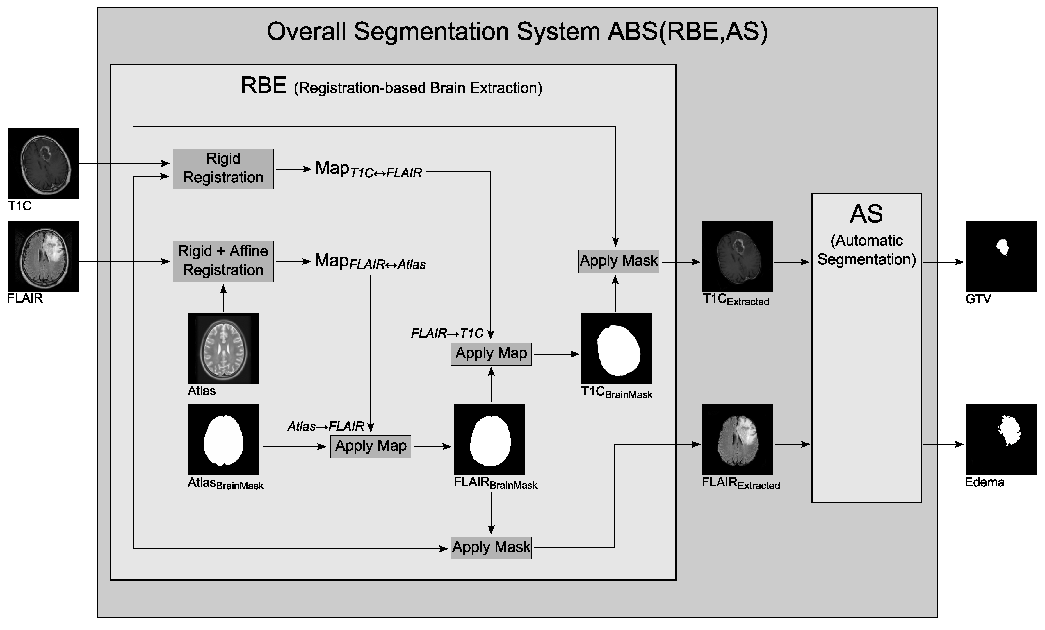
Figure 3 illustrates how RBE identifies brain tissue within the T1C and FLAIR images. Given a volume of T1C images and a corresponding volume of FLAIR images of a patient’s brain, RBE begins by registering the T1C volume to the FLAIR. These two modalities are acquired on the same date and are of the same brain, so rigid registration is sufficient, producing the transformation denoted Map${}_{\mathrm{T}1\mathrm{C}\to \mathrm{FLAIR}}$. After this co-registration step, the volumes are in FLAIR-space.

The FLAIR volume is then registered to the T2-weighted MNI-152 atlas to obtain a transform from the FLAIR-space to atlas-space, for which a brain mask is provided. As the patient brain may not have the same size and shape as the atlas, rigid and affine registration are used to achieve the best possible fit while preserving easy invertibility of the resulting transform, Map${}_{\mathrm{FLAIR}\to \mathrm{Atlas}}$.

We considered a more general class of deformable transformations but found it did not work as well: as tumor and skull had similar pixel intensity, general models tended to be confused by local features such as tumors, which resulted in larger misclassification error.

The segmenter AS has been optimized for unmodified MR images, so the atlas brain mask is transformed into the FLAIR-space to be applied to the original images; this is achieved by inverting Map${}_{\mathrm{FLAIR}\to \mathrm{Atlas}}$, and applying this inverse transformation (Map${}_{\mathrm{Atlas}\to \mathrm{FLAIR}}$) to the atlas brain mask. The resulting FLAIR brain mask is then transformed by the inverse of Map${}_{\mathrm{T}1\mathrm{C}\to \mathrm{FLAIR}}$ to produce a brain mask for the original unregistered T1C volume. The two brain masks, FLAIR${}_{\mathrm{BrainMask}}$ and T1C${}_{\mathrm{BrainMask}}$, are applied to the original FLAIR and T1C volumes to provide skull-stripped brains for AS to segment.

Our empirical studies found that registration of patient FLAIR volumes to the T2 atlas resulted in fewer registration errors than T1C to T1, which is why RBE co-registers the patient’s T1C to the FLAIR, and then registers the FLAIR to the atlas. All registration steps are performed using the freely available BRAINSFit and BRAINSResample command line modules provided with the 3D Slicer application (http://www.slicer.org) [22].

All methods are evaluated over two datasets. The Tumor Dataset contains the T1C and FLAIR brain volumes of 120 unique patients with high grade astrocytoma, as well as corresponding ground truths for edema and GTV (provided by a human expert) for each patient. The Control Dataset contains the T1C and FLAIR brain volumes of 103 control subjects with no apparent brain tumors (these subjects had cancer in other parts of the body and had brain MRIs to rule out metastasis). All scans were done with a 1.5 T magnet, at a spatial resolution of 0.45 mm × 0.45 mm × 5 mm. FLAIR scans had an echo time (TE) of 110 ms and a repetition time (TR) of 9525 ms; the T1C scans had TE ranging from 11 ms to 12 ms and TR ranging from 460 ms to 528 ms. All data was used with Institutional Review Board approval.

3. Results

Each of the skull-stripping methods considered here $e\in${RBE, CBE, BET, HWA, ROBEX} is used as the first step of the ABS(e, AS) segmentation system, all using the same segmenter, AS. Let $V_e\left(p\right)$ be the segmented volume (say GTV) returned when running the ABS(e, AS) on patient p, and $V^{*}\left(p\right)$ be the true segmentation (manually created by an expert). To evaluate the brain extractor e with respect to a patient p, we use the Dice value:

$$D(e,p)=\frac{2|V_e\left(p\right)\cap V^{*}\left(p\right)|}{|V_e\left(p\right)|+|V^{*}\left(p\right)|}.$$

We will then use the average value over a population of patients to evaluate the extractor e. A Dice value of 1 indicates that two regions are identical, while a value of 0 indicates that there is no overlap. To put these scores in perspective, we found the mean Dice agreement achieved between our two experts (MDs) over 19 cases was 0.85 for GTV and 0.79 for edema. This agrees with average inter-operator variability observed in previous studies [1].

3.1. Qualitative Analysis

Infrequently, CBE fails when the active contour meant to shrink to the inner border of the skull does not stop and proceeds into the interior of the brain, as seen in Figure 2a,b; in this case, the region between the contours will be removed and a large amount of tumor tissue is unavailable for the segmenter to find. RBE performs well, much more consistently than CBE. Of the 223 FLAIR volumes considered, only two were poor quality registrations: one in the Tumor Dataset and one in the Control Dataset. These two cases failed to strip parts of the eye sockets, which were then erroneously segmented as tumors.

As previously shown [23], HWA often removes brain tissue along with the skull, but rarely fails to strip non-brain tissue. This helps the performance of ABS(HWA, AS) on the Control dataset but hurts its performance on the Tumor dataset. It occasionally avoids large tumors altogether, only extracting the brain tissue of one hemisphere of the brain due to the presence of a large abnormality in the other. Conversely, BET is much less sensitive, often including the eyes and other non-brain tissues in the stripped image that is provided to the segmenter. This is greatly penalized on the Control dataset, since these areas can then be mistakenly segmented as tumors. ROBEX is also more likely to include non-brain tissue than to strip brain tissue, which means it will often mistakenly include eye sockets and other non-brain areas. Our empirical analysis confirmed that BET, HWA, and ROBEX are problematic within the context of a tumor segmenter.

Figure 4 shows some results of these algorithms, in order to illustrate examples of where each failed.

3.2. Tumor Dataset

On the Tumor Dataset, segmentation errors can occur either due to the skull-stripper or the segmenter; a false positive could occur because a portion of skull that the skull-stripper failed to remove, is mistaken for a tumor, or because the segmenter mis-labels some healthy brain tissue as tumor. A false negative also indicates either a failure of the skull-stripper (when it excludes an area of brain that would otherwise have been segmented as tumor) or the segmenter (when it fails to detect some part of a tumor in the brain tissue).

Figure 5 displays the Dice value results for each of the 120 volumes in the Tumor Dataset. The cases in each chart are sorted such that the Dice value of the RBE method is increasing; RBE is compared separately against CBE, BET, HWA and ROBEX to avoid clutter. In Figure 5a (Top), every point where the dark line is above the light line is an instance where ABS(RBE, AS) outperforms ABS(CBE, AS); conversely, each point where the light line is above the dark line is a case where ABS(CBE, AS) outperforms ABS(RBE, AS). 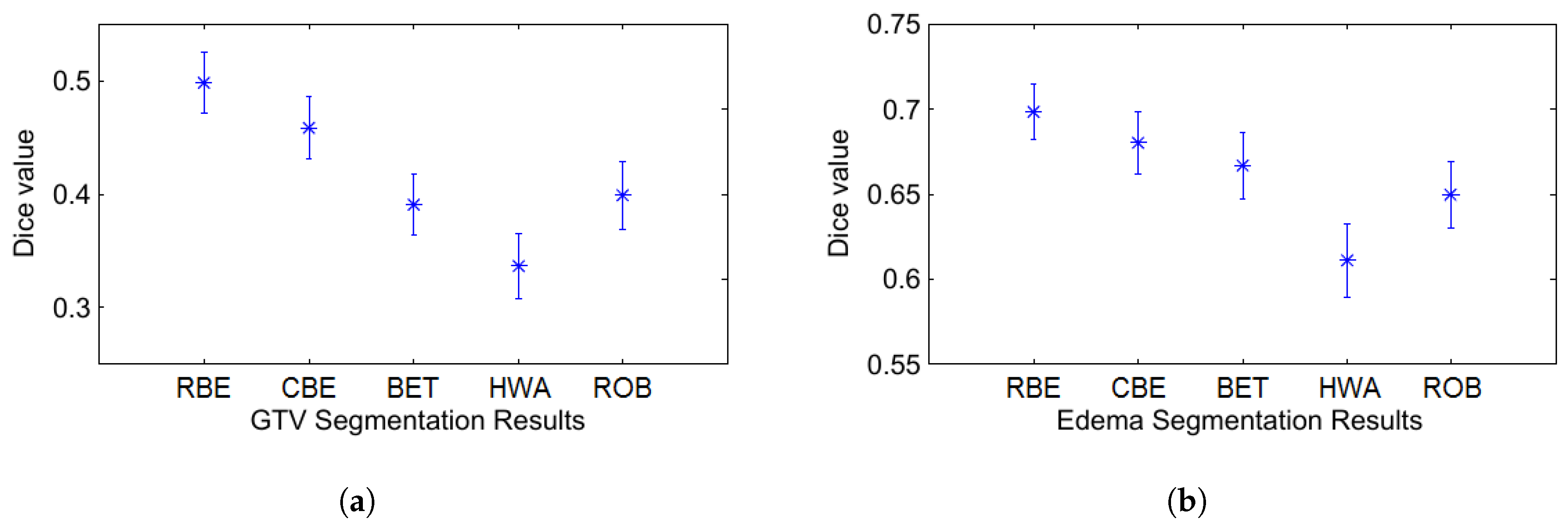To simplify notation in the following discussion, we use e as a shorthand for ABS(e, AS). For the T1C volumes, there are 91 cases where both RBE and CBE produce roughly equivalent segmentations (Dice value within 0.02), four cases where CBE slightly outperforms RBE (mean difference in Dice of 0.04 with a max of 0.06), and 25 cases where RBE performs significantly better than CBE (mean difference in Dice of 0.20 with a max of 0.57). This is easy to see, by noting that there are only a few “bumps” where the light green line is above the dark line, but many places where that green line is far below the dark one. On the T1C volumes overall, RBE achieves a mean Dice value of 0.4983 and CBE achieves 0.4587 (see Figure 6). This difference is significant in a paired t-test at p < 0.01. We observed similar results for the FLAIR volumes, with RBE achieving a mean Dice value of 0.6985 and CBE achieving 0.6803, which is significant at p < 0.05.

With default parameter settings, six patients could not be processed by one or both of BET and HWA (either on the T1C or the FLAIR volume), but a comparison was possible over the remaining 114 patients. For the “process-able” T1C volumes, HWA achieves a mean dice value of 0.3367 and BET achieves 0.3908. Over the corresponding FLAIR volumes, HWA achieves a mean dice value of 0.6112 and BET achieves 0.6669. ROBEX achieves a mean Dice value of 0.4046 over all 120 T1C volumes and a mean Dice value of 0.6396 over the corresponding FLAIR volumes; see Figure 6. In paired t-tests with RBE, each of HWA, BET and ROBEX are significantly worse at p < 0.01, indicating that BET, HWA, and ROBEX are not suitable skull-strippers within the context of a tumor segmenter.

These results were based on the default setting of the various algorithms. We then explored whether they would produce better results, with other settings. We could not change ROBEX, as it was a black box that did not permit any variation in parameters. For BET, we re-ran our study while varying the f parameter for both the Robust and Standard versions of the algorithm, following [3]. For HWA, we adjusted the two parameters: whether or not to use the AtlasCorrection feature, and whether to use Less Restriction or More Restriction. In every case, we found that these modifications produce identical results—that is, they converged to the exact same segmentation (although some modifications led to slightly shorter runtimes, and others, slightly longer). We think this may be because the available BET and HWA parameters are basically designed to reduce the inclusion of extraneous tissue such as neck and shoulder regions (which are almost never present in our datasets), but not to help avoid the skull.

3.3. Control Dataset

While our primary goal is to increase performance of the segmenter on the Tumor Dataset, it is useful to compare the segmenters on a dataset of control patients; on these patients, an ideal tumor segmenter should detect nothing—i.e., 0 voxels of GTV and 0 of edema. In practice, a segmenter with perfect skull-stripping may occasionally find abnormalities due to natural variance in the brain or noise in the MR images. However, with poor skull removal, a segmenter may find abnormalities more frequently.

Over 103 control subject T1C volumes, CBE identified “tumors” in 28 cases, while RBE incorrectly identified tumors in just two cases—one was a failure of the skull-stripper (parts of the eyes were not stripped and were identified as abnormal brain tissue) and the other a failure of the segmenter (some dura mater was segmented). Errors were more common in FLAIR volumes, with CBE falsely identifying 45 cases of edema and RBE falsely identifying 19. For both T1C and FLAIR volumes, the results were significantly different at p < 0.01.

The alternative skull-strippers, BET and HWA, ran to completion on 102 of the 103 cases in the Control Dataset. Over those 102 T1C volumes, the BET-based segmenter produced 85 false positives and the HWA-based segmenter produced 39. Over the corresponding 102 FLAIR volumes, BET resulted in 87 false positives and HWA in 46. ROBEX ran to completion in all 103 cases, and produced 32 false positives over the T1C volumes and 41 false positives over the corresponding FLAIR volumes. See Figure 7.

Once again, varying the parameters did not change the BET and HWA results—they again converged to the same final answer.

3.4. Runtime

It is critical that our segmenter be accurate—i.e., find the correct skull regions. It is also important that it finds these regions quickly; a primary reason for developing strong automatic segmenters is to save clinicians and researchers the time they spend doing manual segmentation; previous studies have shown that experts require an average of 7 to 12 min to segment a single patient [24]. While computer processing time is certainly less valuable than a clinician’s time, it is still important for these methods to be reasonably fast if they are to be used in practice.

We considered the runtime over only the 216 cases that all skull-strippers could process to completion. The mean runtime of the skull-stripping component RBE over these 216 cases (both Tumor and Control datasets) was 98.84 s for each case, compared to 131.16 for CBE (All experiments were performed on an Intel Xeon dual core 2 GHz processor with 8 GB RAM, running Ubuntu). ROBEX was the slowest, taking 154 s on average to complete each skull strip. While BET and HWA are very fast, at 13.74 s and 47.10 s, respectively, the results of the previous sections indicate that they should not be used for tumor segmentation, so we only compare RBE and CBE in the remaining discussion.

Table 1. Runtime breakdown of RBE and CBE in seconds.

RBE      (Total 98.84)
	Step 1: Register FLAIR to Atlas	93.07
	Step 2: Back transform to FLAIR	3.20
	Step 3: Back transform to T1C	2.57
CBE      (Total: 131.16)
	Step 1: Get FLAIR features	0.48
	Step 2: Get T1C features	0.60
	Step 3: Compute initial threshold	28.29
	Step 4: Active Contour propogation	98.92
	Step 5: Back transform to T1C	2.88

shows the time consumption of the major steps of each algorithm; operations common to each, such as co-registration of FLAIR and T1C, are not included. The time taken by the segmentation component AS (acting upon the skull-stripped volumes) is relatively low, requiring only 15.38 s on average. In total (including steps common to both algorithms as well as file conversions and other tasks), ABS(RBE, AS) requires 178 s to skull-strip and segment a tumor patient, while ABS(CBE, AS) requires 215 s, meaning that our registration-based RBE is faster than the active contour approach CBE, as well as producing more accurate segmentation results.

4. Conclusions

Effective skull-stripping is a key component of many automatic tumor segmenters. The experiments presented here demonstrate that a simple atlas-based approach to skull-stripping can achieve segmentation results that are significantly more accurate than an active-contour-based approach. Although the use of rigid registration suggests that the atlas and brain mask may not be perfectly matched to the patient, our two studies show the registration-based approach to be very robust within the context of segmenting tumors in glioma patients, and greatly reduces the spurious segmentation of nonexistent tumors in controls. Moreover, the registration-based approach runs faster than the active contour approach. We anticipate that this system will be a useful tool in the treatment and study of brain tumors.