

Transient Behavior Analysis of Microgrids in Grid-Connected and Islanded Modes: A Comparative Study of LVRT and HVRT Capabilities
Abstract
:1. Introduction
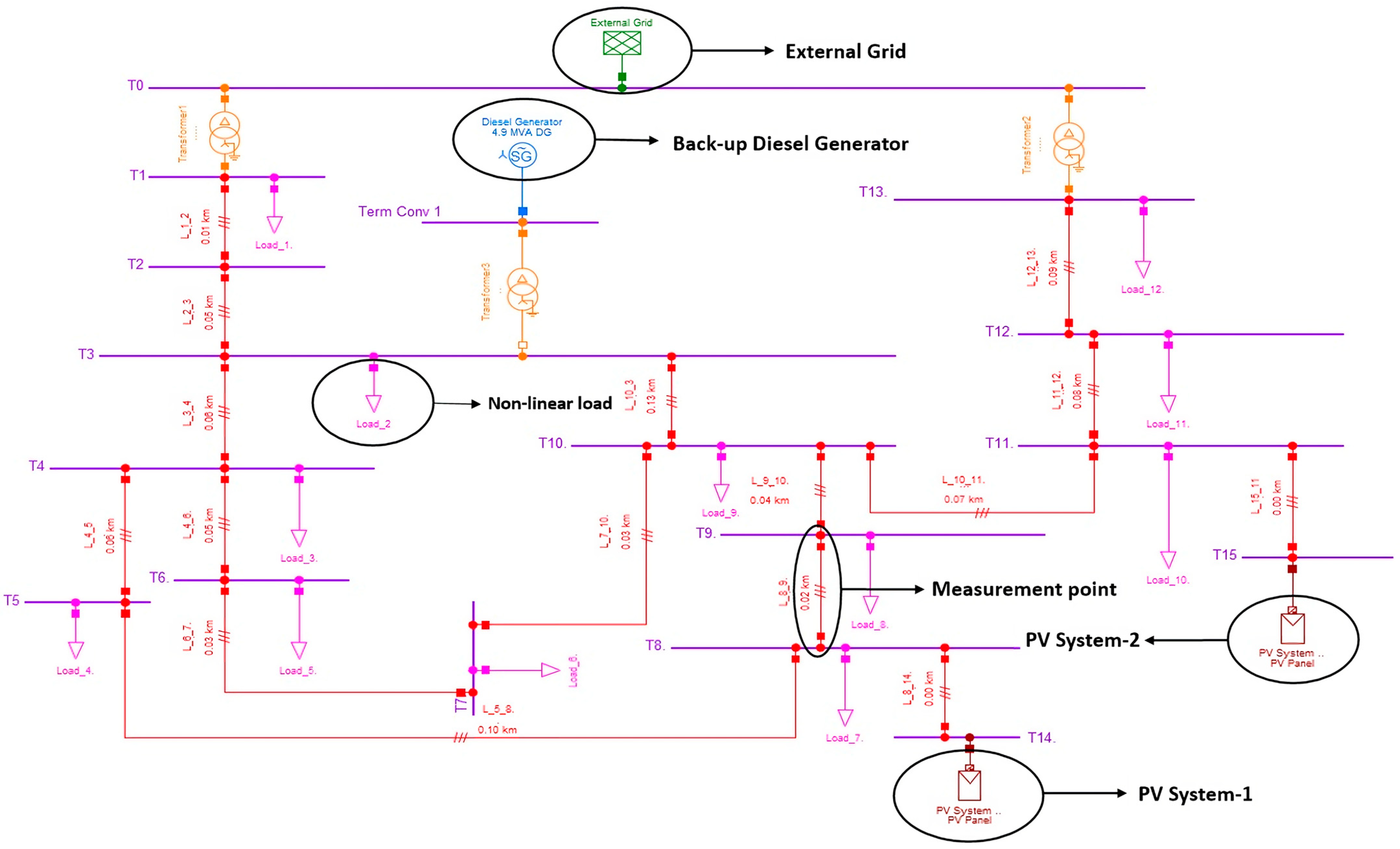
2. Microgrid Model Description
2.1. Lines
2.2. Loads
2.3. Transformers
2.4. Busbars
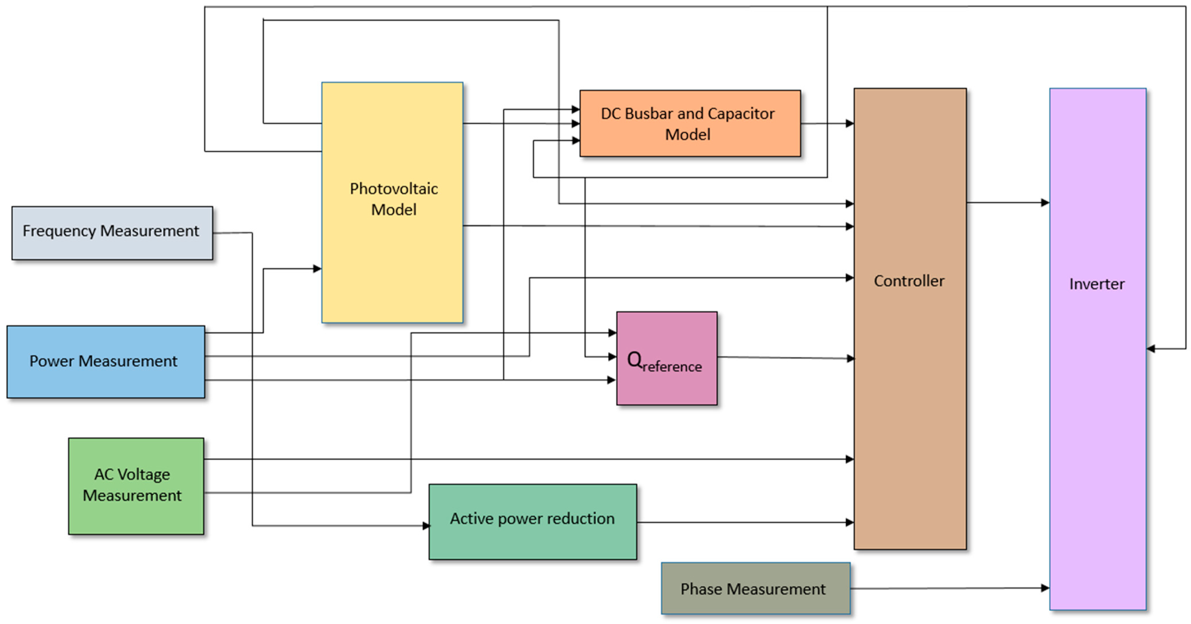
2.5. PV System
2.5.1. Photovoltaic Model
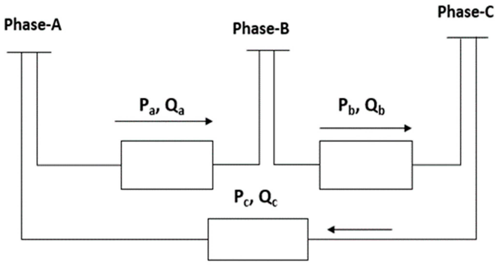
2.5.2. Power Measurement
2.5.3. A.C. Voltage Measurement
2.5.4. Phase Measurement
2.5.5. Frequency Measurement, Active Power Reduction, and DC Busbar and Capacitor Model
2.5.6. Qreference and Controller
2.5.7. Inverter
2.6. Diesel Generator
3. Results and Discussion
3.1. Grid-Connected Mode
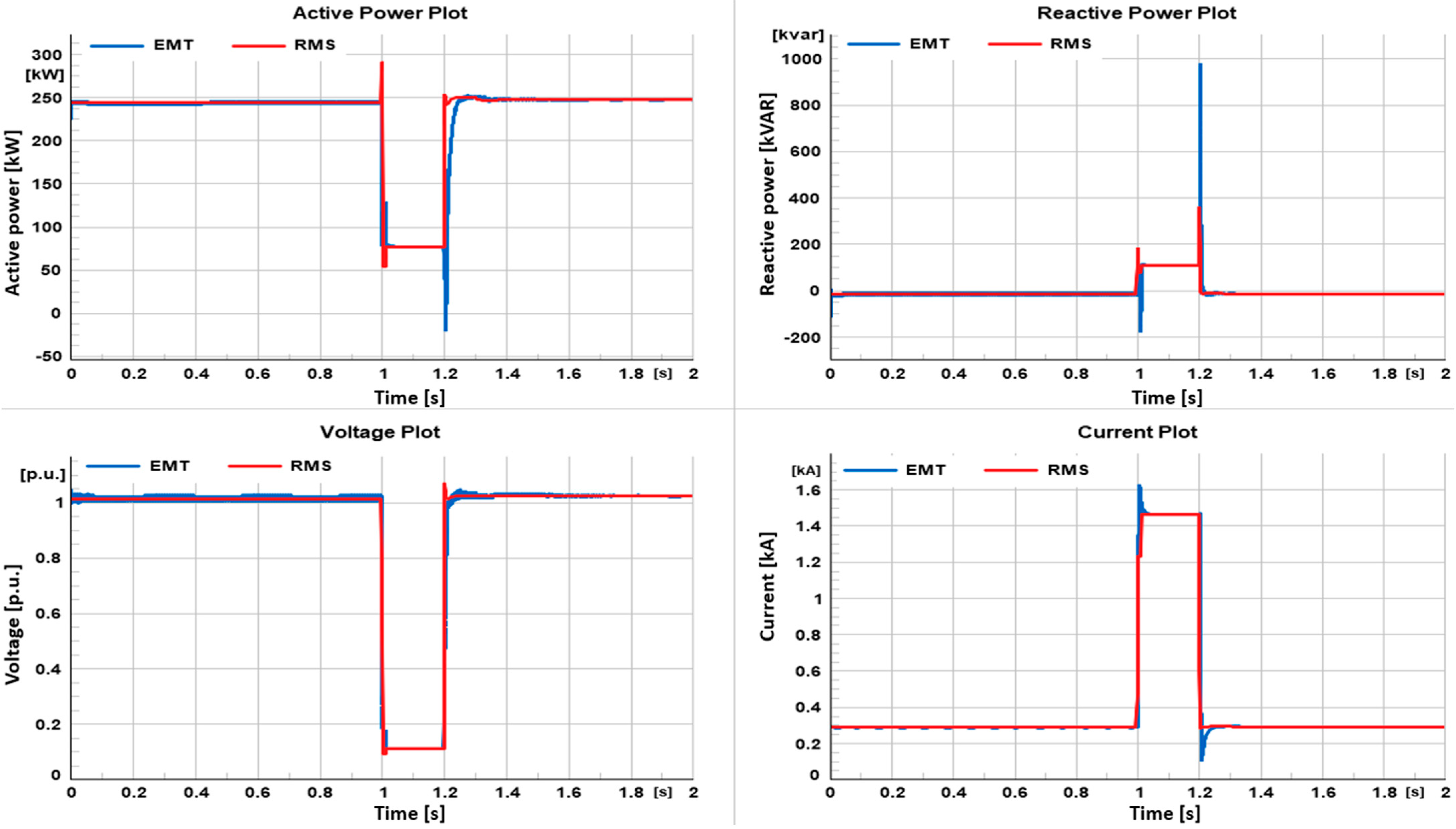
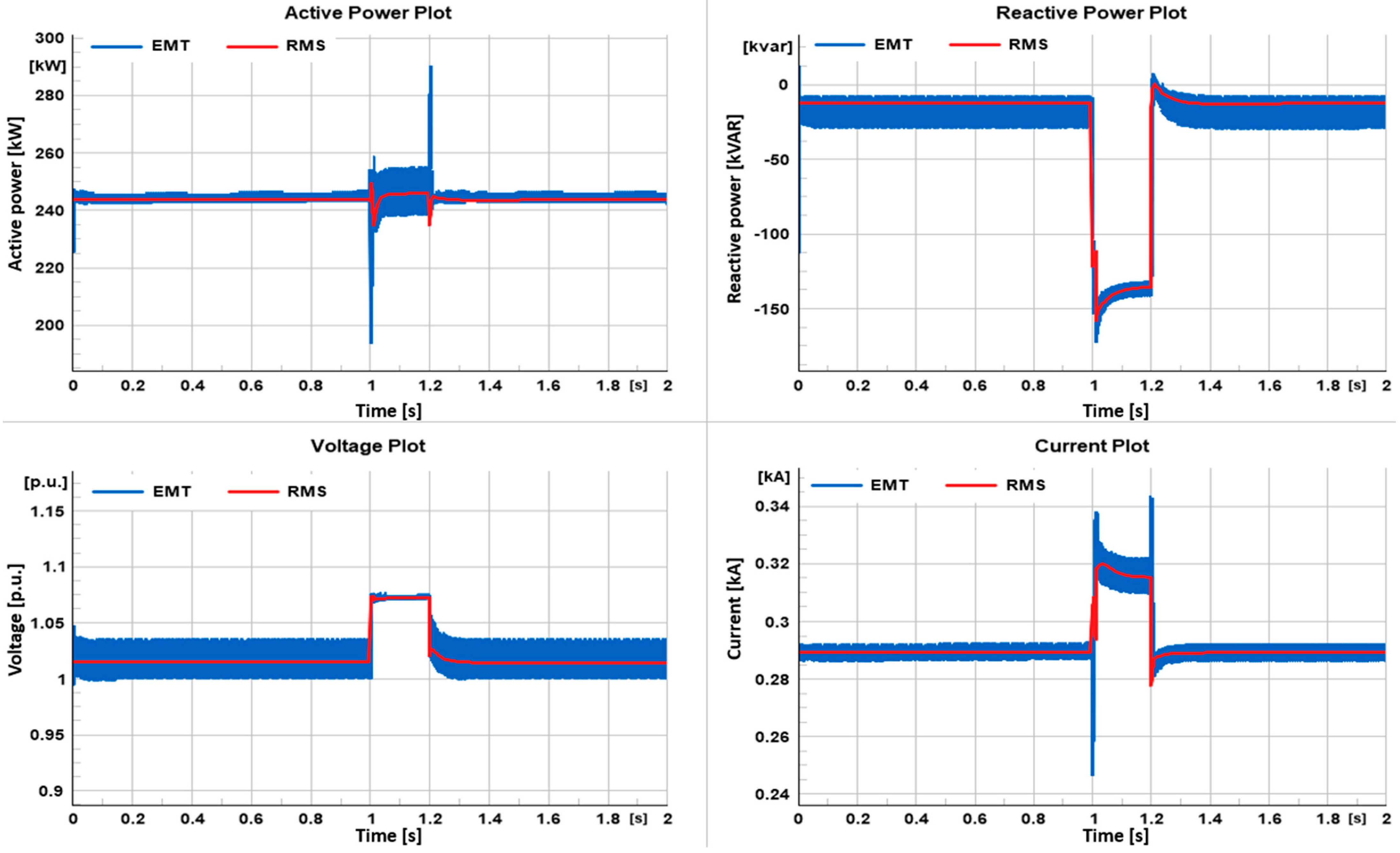
3.1.1. LVRT Case Scenario
3.1.2. HVRT Case Scenario
3.2. Islanded Mode
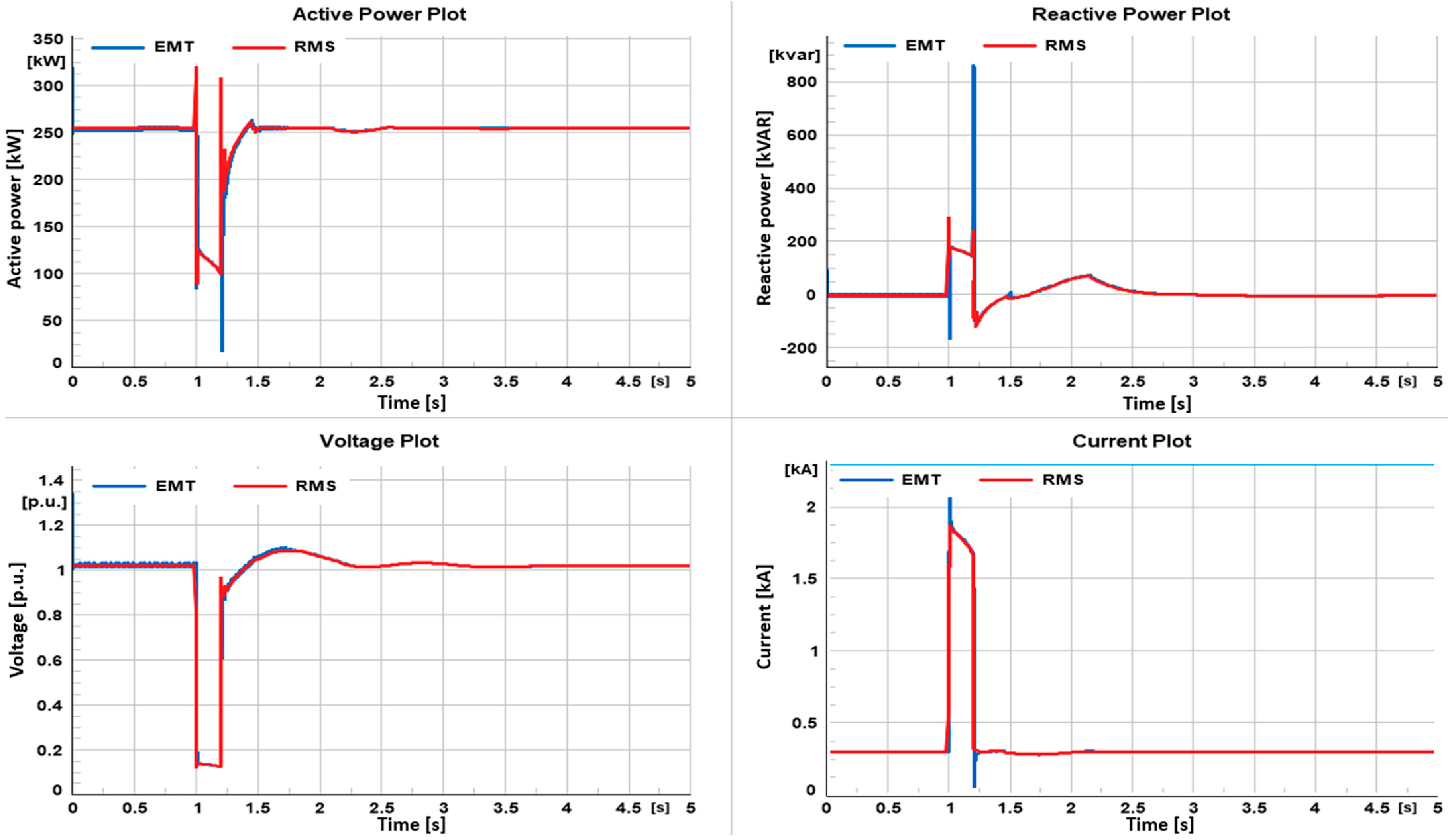
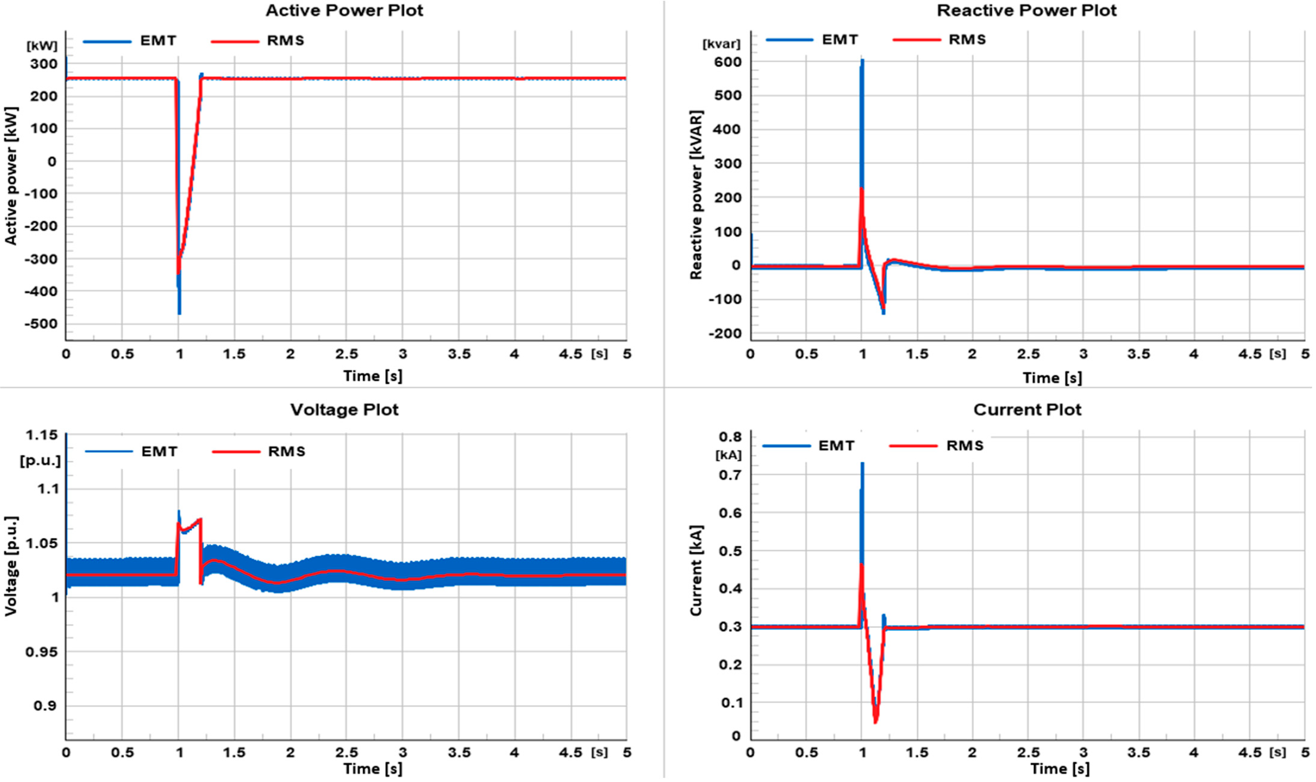
3.2.1. LVRT Case Scenario
3.2.2. HVRT Case Scenario
4. Conclusions
- The microgrid demonstrates the ability to manage LVRT and HVRT events effectively in both grid-connected and islanded modes.
- Notable differences exist in the system’s transient behavior in grid-connected and islanded modes. In particular, the transient recovery time is longer in islanded mode, attributable to the system’s dependence on a single diesel generator for stabilization.
- While computationally more demanding, EMT simulations provide a more nuanced and detailed understanding of high-frequency transient phenomena, validating their utility for advanced studies. RMS simulations, on the other hand, offer a quicker but less granular insight, affirming their appropriateness for generalized, lower-resolution studies.
Author Contributions
Funding
Institutional Review Board Statement
Informed Consent Statement
Conflicts of Interest
References
- Lopes, J.A.P.; Hatziargyriou, N.; Mutale, J.; Djapic, P.; Jenkins, N. Integrating Distributed Generation into Electric Power Systems: A Review of Drivers, Challenges and Opportunities. Electr. Power Syst. Res. 2007, 77, 1189–1203. [Google Scholar] [CrossRef]
- Venkataramanan, G.; Marnay, C. A Larger Role for Microgrids. IEEE Power Energy Mag. 2008, 6, 78–82. [Google Scholar] [CrossRef]
- REN21. Renewables 2022 Global Status Report. Available online: https://www.ren21.net/gsr-2022 (accessed on 29 August 2023).
- Lidula, N.W.A.; Rajapakse, A.D. Microgrids Research: A Review of Experimental Microgrids and Test Systems. Renew. Sustain. Energy Rev. 2011, 15, 186–202. [Google Scholar] [CrossRef]
- Katiraei, F.; Iravani, R.; Hatziargyriou, N.; Dimeas, A. Microgrids Management. IEEE Power Energy Mag. 2008, 6, 54–65. [Google Scholar] [CrossRef]
- Sepasi, S.; Toledo, S.; Kobayashi, J.; Roose, L.R.; Matsuura, M.M.; Tran, Q.T. A Practical Solution for Excess Energy Management in a Diesel-Backed Microgrid with High Renewable Penetration. Renew. Energy 2023, 202, 581–588. [Google Scholar] [CrossRef]
- Reihani, E.; Sepasi, S.; Roose, L.R.; Matsuura, M. Energy Management at the Distribution Grid Using a Battery Energy Storage System (BESS). Int. J. Electr. Power Energy Syst. 2016, 77, 337–344. [Google Scholar] [CrossRef]
- Nasri, M.; Hossain, M.R.; Ginn, H.L.; Moallem, M. Distributed Control of Converters in a DC Microgrid Using Agent Technology. In Proceedings of the 2016 Clemson University Power Systems Conference (PSC), Clemson, SC, USA, 8–11 March 2016; pp. 1–6. [Google Scholar]
- Sarfi, V.; Niazazari, I.; Livani, H. Multiobjective Fireworks Optimization Framework for Economic Emission Dispatch in Microgrids. In Proceedings of the 2016 North American Power Symposium (NAPS), Denver, CO, USA, 18–20 September 2016; pp. 1–6. [Google Scholar]
- Tran, Q.T.; Davies, K.; Sepasi, S. Isolation Microgrid Design for Remote Areas with the Integration of Renewable Energy: A Case Study of Con Dao Island in Vietnam. Clean Technol. 2021, 3, 804–820. [Google Scholar] [CrossRef]
- Foruzan, E.; Algrain, M.C.; Asgarpoor, S. Low-Voltage Ride-through Simulation for Microgrid Systems. In Proceedings of the 2017 IEEE International Conference on Electro Information Technology (EIT), Lincoln, NE, USA, 14–17 May 2017; pp. 260–264. [Google Scholar]
- Davies, K.L.; Tran, T.; Sepasi, S.; Roose, L.R. Distribution Grid Monitoring. U.S. Patent No. 11,146,103, 12 October 2021. [Google Scholar]
- Truong, D.-N.; Thi, M.-S.N.; Le, H.-G.; Do, V.-D.; Ngo, V.-T.; Hoang, A.-Q. Dynamic Stability Improvement Issues with a Grid-Connected Microgrid System. In Proceedings of the 2019 International Conference on System Science and Engineering (ICSSE), Dong Hoi, Vietnam, 20–21 July 2019; pp. 214–218. [Google Scholar]
- Niranjan, P.; Gupta, P.K.; Ahmad, P.; Choudhary, N.K.; Singh, N.; Singh, R.K. Protection Coordination Scheme in Microgrid with Common Optimal Settings of User-Defined Dual-Setting Overcurrent Relays. In Proceedings of the 2023 5th International Conference on Energy, Power and Environment: Towards Flexible Green Energy Technologies (ICEPE), Shillong, India, 15–17 June 2023; pp. 1–5. [Google Scholar]
- Sepasi, S.; Talichet, C.; Pramanik, A.S. Power Quality in Microgrids: A Critical Review of Fundamentals, Standards, and Case Studies. IEEE Access 2023, 11, 108493–108531. [Google Scholar] [CrossRef]
- Machowski, J.; Lubosny, Z.; Bialek, J.W.; Bumby, J.R. Power System Dynamics: Stability and Control, 3rd ed.; Wiley: Hoboken, NJ, USA, 2020; Available online: https://www.wiley.com/en-us/power+system+dynamics%3a+stability+and+control%2c+3rd+edition-p-9781119526360 (accessed on 29 August 2023).
- Cigré; CIRED. Modelling of Inverter-Based Generation for Power System Dynamic Studies; Conseil International des Grands Réseaux Électriques, Congrès International des Réseaux Électriques de Distribution, Eds.; CIGRÉ: Paris, France, 2018; ISBN 978-2-85873-429-0. [Google Scholar]
- Favuzza, S.; Musca, R.; Zizzo, G. A Comparison between RMS and EMT Grid-Forming Implementations in MATLAB/Simscape for Smart Grids Dynamics. In Proceedings of the 2022 IEEE 21st Mediterranean Electrotechnical Conference (MELECON), Palermo, Italy, 14–16 June 2022; pp. 1079–1084. [Google Scholar]
- Acosta, M.A.C.; Soares, B.M.M.; Abildgaard, H.; Parrini, D.R.; Shattuck, A.; Da Costa, I.C.; da Rosa, T. Wind Power Plant Modelling Benchmark of RMS vs EMT Simulation Models for the Electric Reliability Council of Texas (ERCOT) Market. In Proceedings of the 20th International Workshop on Large-Scale Integration of Wind Power into Power Systems as well as on Transmission Networks for Offshore Wind Power Plants (WIW 2021), Online, 29–30 September 2021; Volume 2021, pp. 503–508. [Google Scholar]
- Subedi, S.; Rauniyar, M.; Ishaq, S.; Hansen, T.M.; Tonkoski, R.; Shirazi, M.; Wies, R.; Cicilio, P. Review of Methods to Accelerate Electromagnetic Transient Simulation of Power Systems. IEEE Access 2021, 9, 89714–89731. [Google Scholar] [CrossRef]
- Teodorescu, R.; Liserre, M.; Rodriguez, P. Grid Converters for Photovoltaic and Wind Power Systems; IEEE eBooks; Wiley-IEEE Press: Hoboken, NJ, USA, 2007; Available online: https://ieeexplore.ieee.org/book/5732788 (accessed on 29 August 2023).
- Clark, A.; Mitra, P.; Johansson, N.; Ghandhari, M. Development of a Base Model in RMS and EMT Environment to Study Low Inertia System. In Proceedings of the 2021 IEEE Power & Energy Society General Meeting (PESGM), Washington, DC, USA, 25–29 July 2021; pp. 1–5. [Google Scholar]
- Liu, P.; Zhu, G.; Ding, L.; Gao, X.; Jia, C.; Ng, C.; Terzija, V. High-Voltage Ride-through Strategy for Wind Turbine with Fully-Rated Converter Based on Current Operating Range. Int. J. Electr. Power Energy Syst. 2022, 141, 108101. [Google Scholar] [CrossRef]
- Jayawardena, A.V. Contributions to the Development of Microgrids: Aggregated Modelling and Operational Aspects. Ph.D. Thesis, University of Wollongong, Wollongong, NSW, Australia, 2015. [Google Scholar]
- Safaei, A.; Hosseinian, S.H.; Abyaneh, H.A. Enhancing the HVRT and LVRT Capabilities of DFIG-Based Wind Turbine in an Islanded Microgrid. Eng. Technol. Appl. Sci. Res. 2017, 7, 2118–2123. [Google Scholar] [CrossRef]
- Steinhaeuser, L.; Coumont, M.; Weck, S.; Hanson, J. Comparison of RMS and EMT Models of Converter-Interfaced Distributed Generation Units Regarding Analysis of Short-Term Voltage Stability. In Proceedings of the NEIS 2019 Conference on Sustainable Energy Supply and Energy Storage Systems, Hamburg, Germany, 19–20 September 2019; pp. 1–6. [Google Scholar]
- Conti, S.; Greco, A.M.; Messina, N.; Vagliasindi, U. Intentional Islanding of MV Microgrids: Discussion of a Case Study and Analysis of Simulation Results. In Proceedings of the Automation and Motion 2008 International Symposium on Power Electronics, Electrical Drives, Ischia, Italy, 11–13 June 2008; pp. 422–427. [Google Scholar]
- Perumal, P.; Ramasamy, A.K.; Teng, A.M. Performance Analysis of the DigSILENT PV Model Connected to a Modelled Malaysian Distribution Network. IJCA 2016, 9, 75–88. [Google Scholar] [CrossRef]
- Arraño-Vargas, F.; Konstantinou, G. Development of Real-Time Benchmark Models for Integration Studies of Advanced Energy Conversion Systems. IEEE Trans. Energy Convers. 2020, 35, 497–507. [Google Scholar] [CrossRef]
- Yap, K.Y.; Lim, J.M.-Y.; Sarimuthu, C.R. A Novel Adaptive Virtual Inertia Control Strategy under Varying Irradiance and Temperature in Grid-Connected Solar Power System. Int. J. Electr. Power Energy Syst. 2021, 132, 107180. [Google Scholar] [CrossRef]
- Li, F.; Liu, M.; Wang, Y.; Zhang, X. Research on HIL-Based HVRT and LVRT Automated Test System for Photovoltaic Inverters. Energy Rep. 2021, 7, 405–412. [Google Scholar] [CrossRef]
- D. GmbH. DIgSILENT PowerFactory 2022 MV Microgrid Model; DIgSILENT: Gomaringen, Germany, 2022. [Google Scholar]
- D. GmbH. DIgSILENT PowerFactory 2022 User Mannual; DIgSILENT: Gomaringen, Germany, 2022. [Google Scholar]
- D. GmbH. DIgSILENT PowerFactory 2022 Technical Reference for General Load Model; DIgSILENT: Gomaringen, Germany, 2022. [Google Scholar]
- D. GmbH. DIgSILENT PowerFactory 2022 Technical Reference for 3-Phase, 2-Windings Transformer Models; DIgSILENT: Gomaringen, Germany, 2022. [Google Scholar]
- D. GmbH. DIgSILENT PowerFactory 2022 Technical Reference for Power Measurement; DIgSILENT: Gomaringen, Germany, 2022. [Google Scholar]
- D. GmbH. DIgSILENT PowerFactory 2022 Technical Reference for Voltage Measurement; DIgSILENT: Gomaringen, Germany, 2022. [Google Scholar]
- D. GmbH. DIgSILENT PowerFactory 2022 Technical Reference for Phase Measurement; DIgSILENT: Gomaringen, Germany, 2022. [Google Scholar]
- D. GmbH. DIgSILENT PowerFactory 2022 Technical Reference for Static Generator; DIgSILENT: Gomaringen, Germany, 2022. [Google Scholar]
- D. GmbH. DIgSILENT PowerFactory 2022 Technical Reference for Synchronous Machine Models; DIgSILENT: Gomaringen, Germany, 2022. [Google Scholar]
- D. GmbH. DIgSILENT PowerFactory 2022 Technical Reference for External Grid; DIgSILENT: Gomaringen, Germany, 2022. [Google Scholar]


| Element | RMS | EMT |
|---|---|---|
| Resistor | ||
| Inductor | ||
| Capacitor |
| Cable | Length (km) | Resistance-1,2 Sequence (Ohm/km) | Resistance-0 Sequence (Ohm/km) | Reactance-1,2 Sequence (Ohm/km) | Reactance-0 Sequence (Ohm/km) | Susceptance-1,2 Sequence (μS/km) | Susceptance-0 Sequence (μS/km) | Rated Voltage (kV) | Rated Current (kA) |
|---|---|---|---|---|---|---|---|---|---|
| Line 1_2 | 0.01 | 0.501 | 0.817 | 0.716 | 1.598 | 47.493 | 37.994 | 0.48 | 1 |
| Line 2_3 | 0.045 | 0.501 | 0.817 | 0.716 | 1.598 | 47.493 | 37.994 | 0.48 | 1 |
| Line 3_4 | 0.061 | 0.501 | 0.817 | 0.716 | 1.598 | 47.493 | 37.994 | 0.48 | 1 |
| Line 4_5 | 0.056 | 0.501 | 0.817 | 0.716 | 1.598 | 47.493 | 37.994 | 0.48 | 1 |
| Line 4_6 | 0.045 | 0.501 | 0.817 | 0.716 | 1.598 | 47.493 | 37.994 | 0.48 | 1 |
| Line 5_8 | 0.10 | 0.501 | 0.817 | 0.716 | 1.598 | 47.493 | 37.994 | 0.48 | 1 |
| Line 6_7 | 0.033 | 0.501 | 0.817 | 0.716 | 1.598 | 47.493 | 37.994 | 0.48 | 1 |
| Line 7_10 | 0.032 | 0.501 | 0.817 | 0.716 | 1.598 | 47.493 | 37.994 | 0.48 | 1 |
| Line 8_9 | 0.024 | 0.501 | 0.817 | 0.716 | 1.598 | 47.493 | 37.994 | 0.48 | 1 |
| Line 8_14 | 0.002 | 0.501 | 0.817 | 0.716 | 1.598 | 47.493 | 37.994 | 0.48 | 1 |
| Line 9_10 | 0.04 | 0.501 | 0.817 | 0.716 | 1.598 | 47.493 | 37.994 | 0.48 | 1 |
| Line 10_3 | 0.13 | 0.501 | 0.817 | 0.716 | 1.598 | 47.493 | 37.994 | 0.48 | 1 |
| Line 15_11 | 0.002 | 0.501 | 0.817 | 0.716 | 1.598 | 47.493 | 37.994 | 0.48 | 1 |
| Line 10_11 | 0.07 | 0.51 | 0.658 | 0.366 | 1.611 | 3.172 | 1.28 | 0.48 | 1 |
| Line 11_12 | 0.08 | 0.51 | 0.658 | 0.366 | 1.611 | 3.172 | 1.28 | 0.48 | 1 |
| Line 12_13 | 0.09 | 0.51 | 0.658 | 0.366 | 1.611 | 3.172 | 1.28 | 0.48 | 1 |
| Load | Apparent Power (kVA) | Active Power (kW) | Reactive Power (kVar) | Power Factor |
|---|---|---|---|---|
| Load1 | 200 | 190 | 62.44 | 0.95 |
| Load2 (nonlinear load) | 122 | 100 | 38.08 | 0.82 |
| Load3 | 50 | 47.5 | 15.61 | 0.95 |
| Load4 | 70 | 66.5 | 21.86 | 0.95 |
| Load5 | 35 | 33.25 | 10.93 | 0.95 |
| Load6 | 80 | 76 | 24.98 | 0.95 |
| Load7 | 45 | 42.75 | 14.05 | 0.95 |
| Load8 | 13 | 12.35 | 4.06 | 0.95 |
| Load9 | 72 | 68.40 | 22.48 | 0.95 |
| Load10 | 55 | 52.25 | 17.17 | 0.95 |
| Load11 | 5 | 4.75 | 1.56 | 0.95 |
| Load12 | 75 | 71.25 | 23.42 | 0.95 |
| Names | Positive Sequence Impedance- Reactance/Resistance (p.u.) | Zero Sequence Impedance- Reactance/Resistance (p.u.) | Rated Power (KVA) | Rated Voltage- HV/LV (kV) | Vector Group HV/LV | Copper Losses (kW) | Nominal Frequency (Hz) |
|---|---|---|---|---|---|---|---|
| Transformer-1 | 0.0618/0.0106 | 0.0494/0.0851 | 2500 | 12.47/0.48 | D/YN | 26.5 | 60 |
| Transformer-2 | 0.0618/0.0106 | 0.0494/0.0851 | 2500 | 12.47/0.48 | D/YN | 26.5 | 60 |
| Transformer-3 | 0.0599/0.0014 | 0.04792/0.0011 | 2000 | 10.5/0.48 | D/YN | 2 | 60 |
| Parameter | Values |
|---|---|
| Open-circuit voltage of module at STC (V) | 43.8 |
| MPP voltage of module at STC (V) | 35 |
| MPP current of module at STC (A) | 4.58 |
| Short-circuit current of module at STC (A) | 5 |
| Number of modules in series | 20 |
| Over-sizing factor for PV plant | 1 |
| Name | Unit | Description | Value |
|---|---|---|---|
| Kp | - | Gain of active-power PI controller | 0.005 |
| Tr | s | Measurement delay | 0.001 |
| Tmpp | s | Time-delay MPP tracking | 5 |
| KFRT | - | Gain for dynamic AC voltage support | 2 |
| Kpq | - | Gain of reactive-power PI controller | 0.1 |
| Tpick | s | Pick-up time for fault detection | 0.01 |
| Ulvrt | p.u. | Voltage threshold for LVRT detection | 0.95 |
| Uhvrt | p.u. | Voltage threshold for HVRT detection | 1.05 |
| Tdyn_max | s | Max. duration fault mode | 5 |
| iq_min | p.u. | Minimum reactive current limit | −1 |
| iq_max | p.u. | Maximum reactive current limit | 1 |
| Id_max | p.u. | Maximum active current limit | 1 |
| Title 1 | Title 2 |
|---|---|
| Rated apparent power (MW) | 4.855 |
| Rated voltage (kV) | 10.5 |
| Rated power factor | 0.8 |
| Connection | 3-phase YN |
| Local controller type | Constant V [40] |
Disclaimer/Publisher’s Note: The statements, opinions and data contained in all publications are solely those of the individual author(s) and contributor(s) and not of MDPI and/or the editor(s). MDPI and/or the editor(s) disclaim responsibility for any injury to people or property resulting from any ideas, methods, instructions or products referred to in the content. |
© 2023 by the authors. Licensee MDPI, Basel, Switzerland. This article is an open access article distributed under the terms and conditions of the Creative Commons Attribution (CC BY) license (https://creativecommons.org/licenses/by/4.0/).
Share and Cite
Pramanik, A.S.; Sepasi, S. Transient Behavior Analysis of Microgrids in Grid-Connected and Islanded Modes: A Comparative Study of LVRT and HVRT Capabilities. Clean Technol. 2023, 5, 1287-1303. https://doi.org/10.3390/cleantechnol5040065
Pramanik AS, Sepasi S. Transient Behavior Analysis of Microgrids in Grid-Connected and Islanded Modes: A Comparative Study of LVRT and HVRT Capabilities. Clean Technologies. 2023; 5(4):1287-1303. https://doi.org/10.3390/cleantechnol5040065
Chicago/Turabian StylePramanik, Abrar Shahriar, and Saeed Sepasi. 2023. "Transient Behavior Analysis of Microgrids in Grid-Connected and Islanded Modes: A Comparative Study of LVRT and HVRT Capabilities" Clean Technologies 5, no. 4: 1287-1303. https://doi.org/10.3390/cleantechnol5040065