Heat Recovery Potential in a Semi-Closed Greenhouse for Tomato Cultivation

Abstract

This study first presents the development and the experimental validation of a numerical model of a semi-closed greenhouse using a dynamic thermal simulation. The second objective was to identify the influential parameters on the indoor climate and to calculate the heating demand of the greenhouse. The model reproduced the behavior of a full-scale experimental greenhouse in Carquefou (France). The comparison with experimental measurements recorded over an entire season of tomato cultivation validated the numerical model. The result of the simulated energy consumption was 310 kWh/m²/year with a relative error of 3.5%. The parametric study identified that the evapotranspiration power and ventilation rate were the most influential input variables, accounting for 50% and 32%, respectively, of the heating demand. The most sensitive output variable was indoor humidity. The presence of a thermal buffer zone all around the greenhouse reduced the energy consumption by 48%, and thermal/shading screens reduced it by 30%. The final objective was to assess the amount of heat recovery potential over the year and each week, depending on the energy storage strategy. Around 43 kWh/m²/year can be recovered over the year, leading to a potential energy savings of 24%.

1. Introduction

Construction and operating costs are two important criteria to define an optimal greenhouse [1,2]. The design of a greenhouse is a demanding task because many constraints must be considered, such as the variation of the plants’ needs according to their different phases of growth, the protection of the plants from extreme climatic conditions, or the choice of construction materials that must guarantee an ideal thermal and hygric environment. Greenhouses accelerate agricultural cultivation under favorable weather conditions and protect the cultures under adverse ones. They enable the control of air temperature, relative humidity, and CO₂ concentration for optimal plant growth [3]. In particular, it is necessary to heat the greenhouse when outdoor temperatures are below 10 °C. Ventilation must be sufficient to avoid excessive temperatures and/or humidity ratios inside the greenhouse, and it is necessary to cool the greenhouse when the outdoor temperatures are above 27 °C [4]. The relative humidity is an important variable to control for plants’ growth. Indeed, greenhouse growers are often forced to evacuate moisture by increasing the ventilation flow rate in conventional greenhouses. They act on the openings, and at the same time, they increase the heating power to compensate the heat losses due to higher ventilation rates. Hou et al. concluded that the development of crops also affects the indoor air temperature, relative humidity, and solar radiation inside the greenhouse [5].

In the literature, indoor hygrothermal behavior in greenhouses has often been examined by numerical simulations. Depending on the climatic conditions and the parameters of the greenhouse components, the numerical modeling can be either a steady-state energy calculation or a transient thermal simulation. Several studies have been successfully conducted using TRNSYS [6] to understand, analyze, and predict indoor climate and energy consumptions. Mashonjowa et al. modeled the thermal performance of a naturally ventilated greenhouse in Zimbabwe [4]. Rasheed et al. simulated the energy-saving options of multi-span greenhouses without taking into account the presence of the plants [7]. Different parameters are tested as the presence of a thermal screen, the glazing type, the greenhouse orientation, and the level of thermal inertia. The authors found that changing the northern glazed wall by an opaque one would only bring 5% energy savings. In another study, TRNSYS software shows high flexibility and capacity to simulate the effect of different thermal screen materials on the energy requirement of greenhouses [8]. The results showed that a multi-layer thermal screen can reduce the heating energy demand by 20% in comparison with a thermal screen made of polyester. In the study conducted by Patil et al., TRNSYS was found to successfully simulate certain types of energy storage systems inside a greenhouse [9]. Thermal modeling of a geothermal system was performed using TRNSYS with results close to the experimental data by Chargui et al. [10]. Candy et al. modeled a greenhouse built in a cold and remote area in Nepal [11]. Using TRNSYS, they were able to describe the variation of the indoor humidity and temperature of the greenhouse, by modeling the phenomenon of evapotranspiration that occurs when solar radiation hits the leaves of the plants. Three types of greenhouses exist: conventional, semi-closed, and closed. The performances of the three types were compared and analyzed using TRNSYS software by Banakar et al. [12]. The results showed that the thermal demand in the closed greenhouse compared with the conventional greenhouse was about twice lower, and the cooling requirement in this type of greenhouse was about three times higher than in the conventional greenhouse. A semi-closed greenhouse with a good ventilation management seemed to be the best greenhouse type in terms of energy consumption. Chahidi et al. developed a dynamic energy model in the EnergyPlus environment of a high-efficiency greenhouse located in northwestern Italy [13]. The studied greenhouse was equipped with a ground-coupled heat pump, borehole heat exchangers, and an electric energy production by photovoltaic panels. The authors concluded that the model could be useful for analyzing new strategies of energy management and for optimizing the greenhouse system. A typical Mediterranean greenhouse located in Almería, in the southeast of Spain, was successfully modeled using mass and energy balances in the object-oriented Modelica language and the Dymola library [14]. A sub-model was developed and validated independently for each quarter of the greenhouse. The components were then linked, and the whole model was validated based on the data obtained from in situ measurements. Constantino et al. proposed an energy model for greenhouse dynamic simulation that considered the building’s dynamic hygrothermal behavior, as well as the reaction of the grown crops depending on changes in solar radiation [15]. When the crops grow, they create a shade on the crops behind them. A variable shading factor was used to take this phenomenon into account. They employed this model as a tool to adequately address energy efficiency optimization in mechanically ventilated greenhouses. The evaluation of heat and mass transfer functions in an innovative solar greenhouse with thermal screen was highlighted by Taki et al. using numerical and experimental approaches [16]. Results on a greenhouse employing thermal screens at night in autumn demonstrated that such an operation could reduce the consumption of fossil fuels by up to 58%, minimizing costs and air pollution due to fuel burning. A dynamic model calculating the air temperature and humidity was developed by Van Beveren [17]. The model was validated by comparison with experimental measurements. The authors defined the upper and lower limits of the indoor temperature and humidity in the greenhouse to have an optimal energy consumption. However, heating, cooling, and ventilation systems are not considered in the optimization. Esen and Yuksel conducted an experimental investigation of the indoor climatic conditions in a greenhouse heated by biogas, solar, and ground energy in Elazig, Turkey [18]. According to their experimental tests, a biogas reactor could be used as an efficient heating device to maintain a temperature of around 23 °C and reduce the environmental impact. Another system based on an earth pipe air heat exchanger (EAHE) for heating the air in a closed greenhouse was studied by Hepbasli [19]. It included modeling, analysis, and evaluation without experimental validation. As the reference ambient temperature increased inside the greenhouse from 0 to 18 °C, the exergy efficiency of the entire EAHE system dropped from 19.18% to 0.77%. In order to estimate the air temperature, vapor pressure, and canopy temperatures in a greenhouse for flowers, Kumar et al. created a simplified dynamic model [20]. The model’s sensitivity analysis revealed that the size of the side openings and the angle of the roof vent had a significant impact on the model’s performance. Berroug et al. examined the thermal properties of the northern wall of an east–west-oriented greenhouse containing a phase change material (PCM) [21]. Due to the integration of a PCM having a thickness of 4 cm in the northern wall as a storage medium, there is an increase of 6 to 12 K in plant and indoor air temperature, a decrease of 4 to 5 K in cover temperature at night, and a relative humidity decrease of 10 to 15%. A dynamic model was created by Mobtaker et al. to analyze six greenhouse shapes from the perspective of solar radiation availability, including uneven span, even span, single span, and arch type [22]. The greenhouse’s indoor air, ground surface, and northern wall temperatures are predicted by the model. They found that an east–west-oriented greenhouse with a single span received roughly 8% more solar energy over the entire year. Additionally, it was shown that placing a brick wall on the greenhouse’s northern wall can reduce the radiation energy loss.

Table 1. Research studies about modeling and experimental studies on greenhouses.

Authors	Case Study	Numerical Model	Experimental Validation and Presented Measurements
Rasheed et al. [7,8]	Building energy and simulation model for analyzing energy-saving options of multi-span greenhouses	Transient model using TRNSYS	20 days 20–29 August, 1–10 December
Banakar et al. [12]	Energy performance investigation of three types of greenhouses: conventional, semi-closed, and closed	Transient model using TRNSYS	4 days 17 January, 15 May, 17 July, and 14 November
Chahidi et al. [13]	Study of a greenhouse equipped by a ground with heat pump and photovoltaic panels in roof	Simulations with EnergyPlus	56 days 1–31 March, 20 August to 13 September
Costantino et al. [15]	Energy consumption of a new fully mechanical ventilation-controlled greenhouse	Model workflow	31 days July
Taki et al. [16]	Six geometries of semi-solar greenhouse are analyzed	MATLAB software	2 days 2 November and 30 November
Van Beveren et al. [17]	Development and validation of a dynamic air temperature model for greenhouse in order to optimize energy consumption	PROPT–MATLAB Optimal Control Software	7 days 13 to 20 April
Mobtaker et al. [22]	Analysis of the greenhouse shape effect on heat losses and solar radiation gains	MATLAB Software	1 day 29 November

summarizes the previously cited numerical studies that were experimentally validated. This table clearly shows a lack of detailed experimental data for model validation covering the entire cultivation season. According to this literature review on greenhouse research, the design regarding the geometry and orientation of glazed surfaces as well as adequate selection of envelope materials enables the optimization of the energy consumption while ensuring favorable conditions for the plants’ growth. However, greenhouses generally remain very energy demanding and highly dependent on fossil fuels, leading to a strong impact on the environment. Nevertheless, greenhouse gas emissions are limited because a large amount of CO₂ produced to heat the greenhouses is consumed by the plants during photosynthesis. Soil-less crops grown in heated greenhouses are very productive while using few or no chemical inputs. Although they are economical in terms of phytosanitary products and water, the overall balance is unsatisfactory because of their higher energy demand. Therefore, a research effort is still necessary to design greenhouses that consume less fossil fuel. It is becoming necessary in the context of the recent and continuous increase in energy cost. The design of new energy-efficient greenhouses requires the use of models that are able to accurately reproduce the hygrothermal behavior of a greenhouse, in order to serve as a parametric analysis tool for choosing various envelope and system characteristics. Previous studies showed that the important input parameters seem to be the greenhouse’s geometry and materials; the influential variables are solar irradiance, ventilation rates, internal heat, and humidity gains by the plants; and the main output variables are temperature, humidity ratios, and energy consumptions.

This article intends to provide a contribution to both experimental and numerical aspects. A complete database on an entire season of a full-scale experimental greenhouse is presented and used as a reference for the development of a numerical twin. As it is widely used by the scientific community, the commercial software TRNSYS was chosen to model the experimental CTIFL greenhouse. The following sections describe the experimental greenhouse, the model, the validation process, and the determination of influential parameters using a parametric study. The contributions of heat losses through the envelope, due to evapotranspiration and ventilation, are first investigated. The effects of the glazing type, thermal inertia, thermal buffer zone, and thermal/shading screens are assessed. Thermal and shading screens are now commonly used in semi-closed greenhouses. A possibly hot thermal zone is created above the screens. A lot of heat can be recovered and stored. Depending on the storage duration, different storage systems can be employed. A previous study reviewed the storage systems available depending on the storage time [23].

Table 2. Review summary on energy storage systems.

Storage Time	Article	System	Power	Energy Storage Capacity	Round-Trip Efficiency
Very low	Rahman et al. [24]	Flywheel	20 MW	5 MWh	90%
	Barnhart and Benson [25]	Batteries	Not provided	4–12 h	75–90%
	Odukomaiya et al. [26]	Batteries	kW–MW scale	180–1800 MJ/m3	63–90%
	Barnhart and Benson [25]	Flow batteries	Not provided	4–12 h	64–71%
Low	Hunt et al. [27]	PHES	100 MW	1 day to several years	Not provided
	Cavazzini [28]	PHES	Over 7400 MW	Not provided	65–80%
	Pujades et al. [29]	PHES	Not provided	Up to 2 days	Not provided
	Connolly et al. [30]	PHES	360 MW pump 300 MW turbine	2 GWh	85% (92% pumping 92% generating)
	Odukomaiya et al. [26]	PHES	GW scale	0.72–7.2 MJ/m3	65–87%
Medium	Olabi et al. [31]	CAES	3 kW to 1 GW	100 kWh–1 GWh	40–70%
	Odukomaiya et al. [26]	CAES	kW–GW scale	7.2–21.6+ MJ/m3	30–70%
	Tallini et al. [32]	CAES	33–100 kW	Not provided	Not provided
	Bi et al. [33]	CAES-PHES	Not provided	Not provided	21.7–22.6%
	Odukomaiya et al. [26]	CAES-PHES	3 kW	2.46–3.59 MJ/m3	66–82%
	Dib et al. [34]	AA-CAES	23.5 kW	188 kWh 54.6 MJ/m3	33.7%
	Kandezi et al. [35]	LAES	5300 kW	762 MJ/m3	65.7%
	Georgiou et al. [36]	LAES	12 MW	50 MWh	55%
	Steinmann et al. [37]	PTES	Multi-MW	Up to 200,000 m3	70%
	Mercangöz et al. [38]	PTES	50 MW	1 MWh	65%
	McTigue et al. [39]	PTES	2 MW	200 MJ/m3	70%
	Georgiou et al. [36]	PTES	2 MW	11.5 MWh	75%
	Siemens Gamesa [40]	PTES	100 MW	130 MWh	50%
High	Hu et al. [41]	Hydrogen and synthetized gas	7 kW to 1 MW	2360–4600 MJ/m3	19–45%

summarizes the results of this literature review. Flywheel, batteries, and flow batteries had very low storage times compared with the targeted application. The losses were too high if the heat was kept longer. Pumped hydro energy storage (PHES) can also be considered as a low-time storage system between 1 and 30 h. Compressed air energy storage and advanced adiabatic compressed air energy storage systems (CAES and AA-CAES), liquid air energy storage (LAES), and pumped thermal energy storage (PTES) can become interesting solutions for longer storage times between 1 week and 1 month. If a longer storage time is needed, hydrogen and synthetic gas production can be envisaged. The power and the storage capacity of the systems grossly increase as the storage time increases. The round-trip efficiency is the multiplication of the conversion efficiency from the source to the storage by the conversion efficiency from the storage to the use. It decreases as the size, power, and capacity of the storage increase. According to this non-exhaustive list, energy storage systems exist in various forms and could be employed in the greenhouse energy management system. The final objective of the present article is to evaluate the amount of energy recoverable over the year and over a week that could be stored and reused to reduce energy consumptions.

2. Materials and Methods

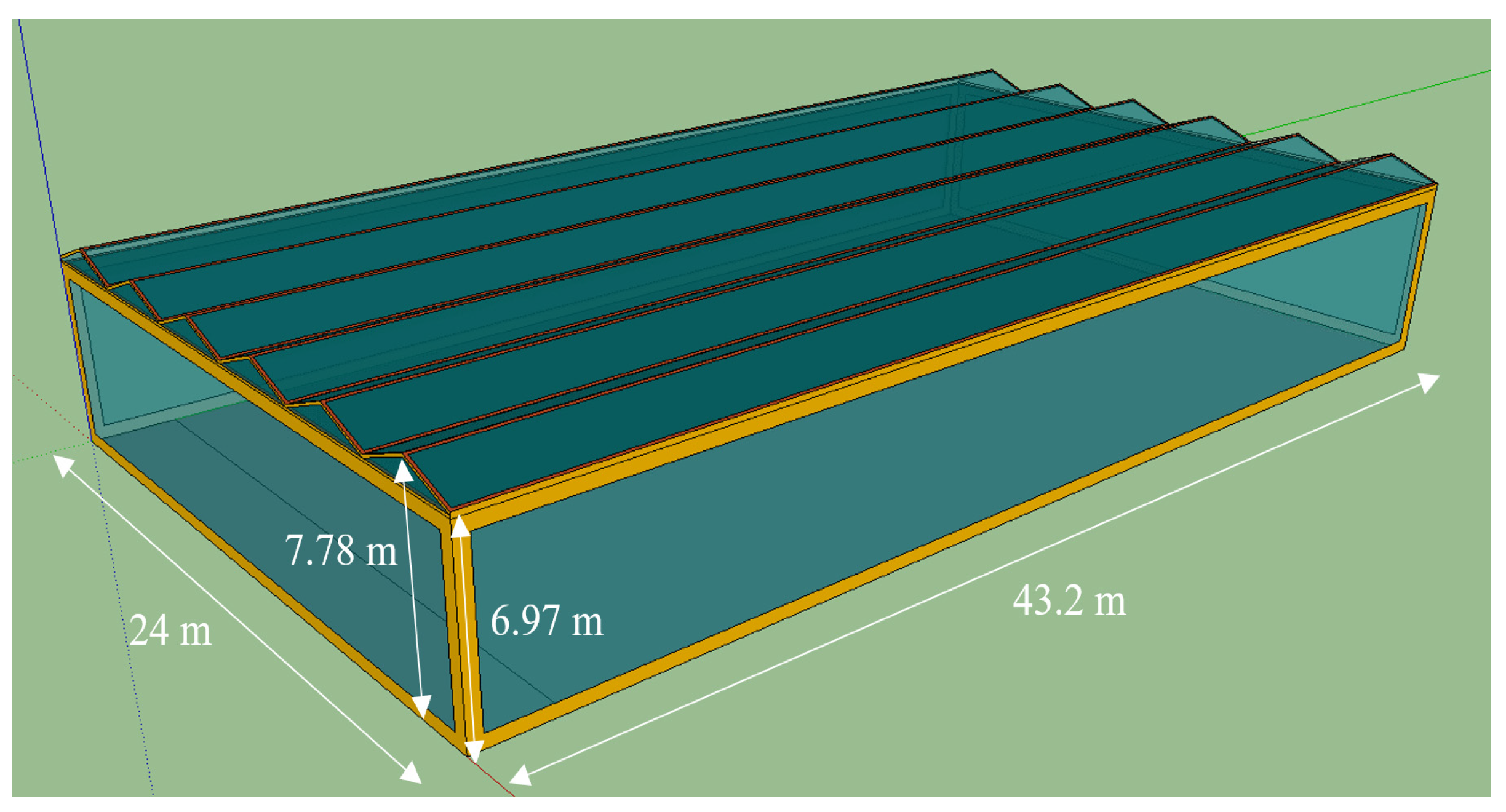
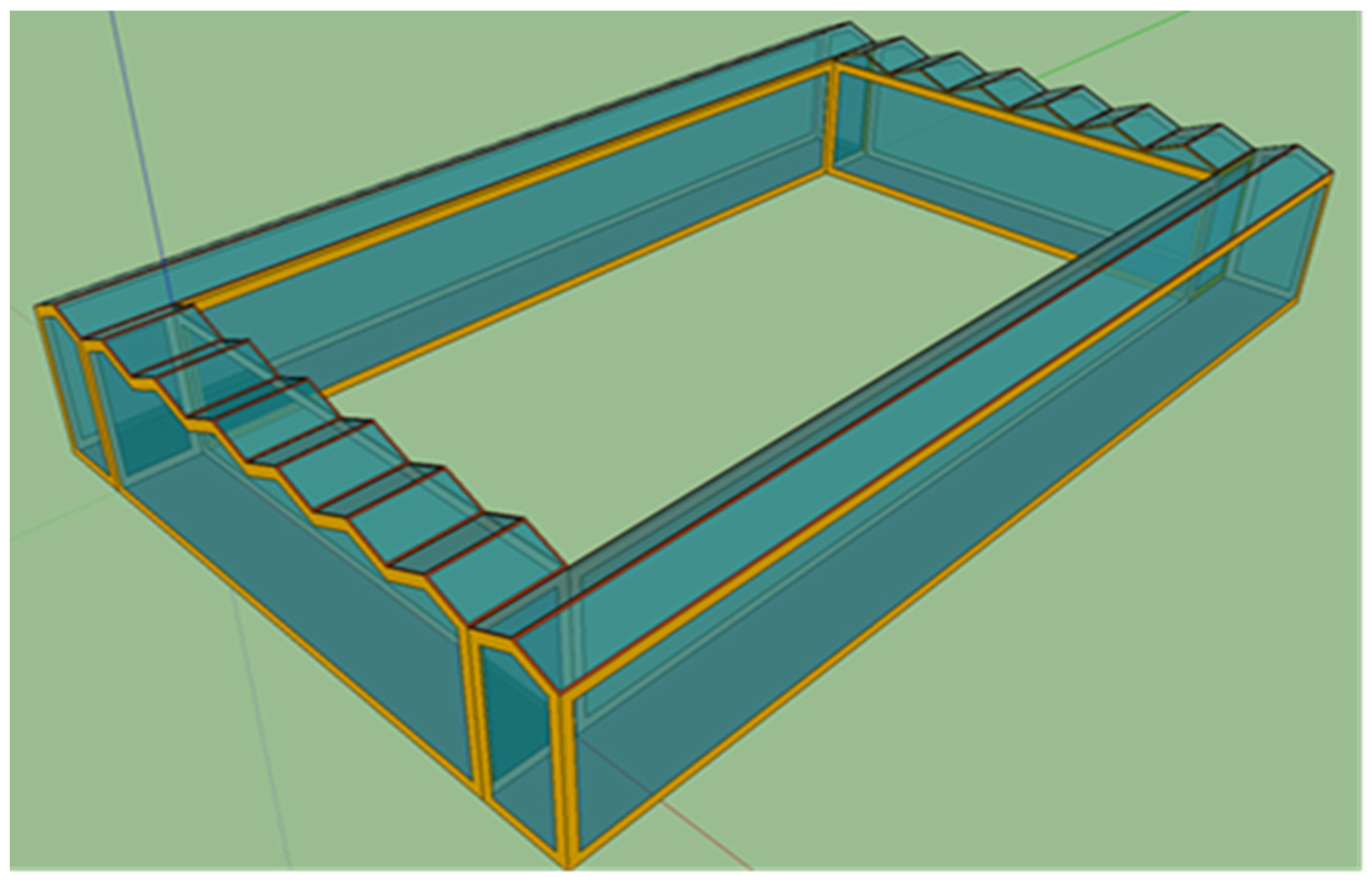
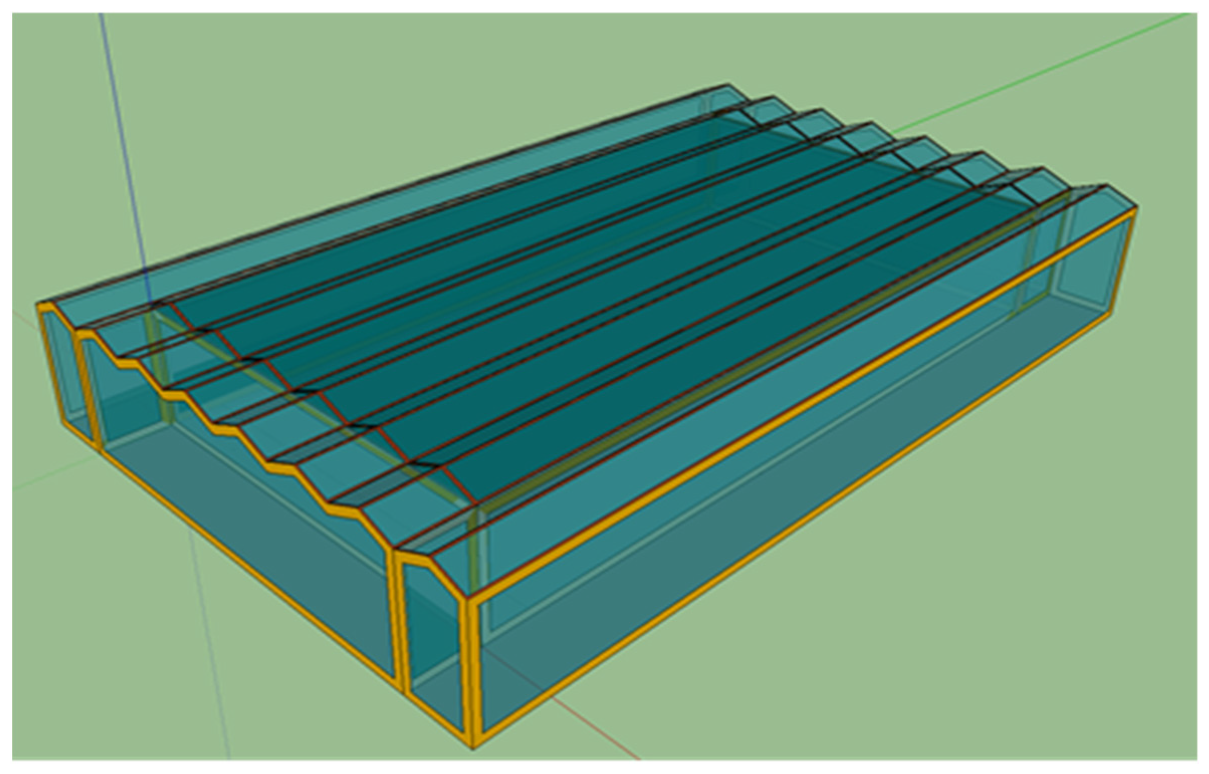
2.1. Greenhouse Geometry and Materials

The CTIFL (Centre Technique Interprofessionnel des Fruits et Légumes) semi-closed greenhouse is a six-bay Venlo-type greenhouse used for the cultivation of tomatoes. It is located in Carquefou, in the west of France, near Nantes. The climate is oceanic. Figure 1 shows the CTIFL experimental greenhouse drawn with Sketchup 3D. It consists of six chapels having the following dimensions: 4.00 m wide, 43.20 m long, 7.78 m ridge height, and 6.97 m eave height. The interior floor area is 1037 m².

The equipment installed in the CTIFL greenhouse enabled the maintenance of an indoor environment suitable for the plants’ growth. The heating and ventilation systems controlled the temperatures between 13 °C and 30 °C and the relative humidity between 60% and 80%.

Figure 2 shows the thermal buffer zone that surrounds the greenhouse. With a width equal to the one of a chapel (4 m), it served on one hand for the circulation of employees and equipment, and on the other hand, it created a thermal buffer zone between the indoor climate and the outdoor climate to reduce horizontal heat exchanges.

In Figure 3, the thermal buffer zone and the greenhouse compartments are merged. Two thermal zones were created inside the greenhouse, below and above the thermal and shading screens both installed on the same cables at eave height. The shading screen was rolled out over the crops during strong solar radiation, and the thermal screen was rolled out at night to limit heat losses during cold nights. Inside the thermal buffer zone, four sub-zones (north, south, east, and west) were created.

The materials used in the models have the thermophysical characteristics shown in

Table 3. Properties of materials and ground composition.

Element	Composition	Thickness (m)	Properties
Frame wall	Aluminum	0.05	ρ = 2700 kg·m−3 C = 860 J·kg−1·K−1 λ = 256 W·m−1·K−1 hci = 3 W·m−2·K−1 hce =17 W·m−2·K−1
Window	Glass tempered	0.004	g-value = 0.9 τsol = 0.896 ρsol = 0.080 τL= 0.907 hci = 3 W·m−2·K−1 hce = f(V, Text,Tglass) as presented in Section 2.2.1
Concrete floor	Concrete	0.250	ρ = 2200 kg·m−3 C = 880 J·kg−1·K−1 λ = 0.331 W·m−1·K−1 hci = 3 W·m−2·K−1
Ground floor	Soil White tarpaulin	0.250 0.005	For soil ρ = 3200 kg·m−3 C = 840 J·kg−1·K−1 λ = 2.4 W·m−1·K−1	For tarpaulin ρ = 120 kg·m−3 C = 484 J·kg−1·K−1 λ = 0.04 W·m−1·K−1
			hci = 3 W·m−2·K−1
Themal screen XLS-10 ULTRA REVOULUX	Aluminium strips	0.004	Energy savings = 47% Direct light transmission = 85% Diffuse light transmission = 76%
Shading screen XLS-35F HARMONY REVOULUX	Polyster	0.004	Energy savings = 15% Direct light transmission = 65% Diffuse light transmission = 63%

. A ground model was used to define the soil temperature at a depth of 25 cm, at which the variations between winter and summer were modeled by a sinusoidal temperature profile based on the average temperature of the past 30 years. The average soil temperature over the 10-month period was equal to 12.4 °C, the minimum soil temperature in January was equal to 6.7 °C, and the maximum soil temperature in July was equal to 16.7 °C. The simple glazing type was taken from the TRNSYS database. Input files allowed the consideration of the variation of the optical and energetic coefficients of transmission, absorption, and reflection of the glazing according to the orientation of the direct solar radiation. The frames chosen in the simulations were made of aluminum. The thickness, composition, and heat conductance of each part of the greenhouse envelope and the characteristics of the glazing are listed in Table 3. The ground was covered by a white tarpaulin acting as a thin insulation layer in order to limit the hygrothermal transfer between the ambiance and the soil. For the calculation of the radiative heat exchange coefficient, the internal calculation of TRNSYS was used. It was based on the form factors of the surfaces using the standard model Starnet (or Star Network). This model simply uses a ratio of surfaces for the distribution of infrared radiation exchanges.

2.2. Modeling of Specific Phenomena

Other thermal phenomena are not correctly considered in the existing model library of TRNSYS and require an independent calculation. They are modeled by open “Equation” modules allowing the description of any behavior. The following three specific phenomena are described in Section 2.2.1, Section 2.2.2 and Section 2.2.3:

• The convection heat exchange coefficient with outdoor air for transparent walls (the heat exchange by thermal infrared radiation being low because of the high reflectivity of the glass greenhouse surfaces, no specific coefficient is needed);
• The evapotranspiration by plants as heat and moisture gain;
• The air infiltrations in a greenhouse-type structure and the voluntary ventilation by a specific management of the openings.

2.2.1. External Heat Exchange Coefficient by Convection

For transparent greenhouse walls, the external convective heat transfer coefficient h can be modeled based on measurements by Yazdanian and Klems taken at the Mobile Window Thermal Test (MoWiTT) facility [42]. This exchange coefficient depends on the wind speed at a certain height above the ground and the temperature difference between the outer wall surface and the outside air. In addition, the model distinguishes between the windward and leeward exposure of the opening. It applies to vertical surfaces of moderate height and is not suitable for rough surfaces. Equation (1) presents the calculation of the convective heat exchange coefficient between the transparent walls of the greenhouse and the outdoor environment.

$$h_{ce}=\sqrt{{\left(0.84\Delta T_e{}^{\frac{1}{3}}\right)}^2+{\left(a{V}_z{}^b\right)}^2}$$

(1)

with

• $\Delta T_e$ = $T_{glass}-T_{ext}$;
• $V_z$ = the vertical component of the wind speed (m/s);
• a = 2.38 on the windward side and a = 2.86 on the leeward side;
• b = 0.89 on the windward side and b = 0.62 on the leeward side.

2.2.2. Evapotranspiration

Several empirical methods have been developed to estimate evapotranspiration by plants and their substrate as a function of different climatic variables. The equations are often subject to local adjustments and have shown a limited global validity. For a greenhouse radiative transmittance of 65%, Hamer proposes a formulation to calculate the evapotranspiration rate Tr in W·m⁻² using the outdoor solar radiation Re (W·m⁻²) and the vapor pressure deficit VPD (kPa) [43].

$$\mathrm{Tr} =0.174\cdot \mathrm{Re}+\frac{693.6\cdot (1-\exp \left(0.00225\cdot \mathrm{Re}\right)\cdot \mathrm{VPD}}{f\left(\mathrm{VPD}\right)}$$

(2)

with

$$f\left(\mathrm{VPD}\right)=\frac{4}{(1+255\cdot \exp {\left(-5.55\cdot \mathrm{VPD}\right)}^{0.25}}$$

(3)

Another model based on incident solar radiation on the crop Ri (W·m⁻²) and the VPD (kPA) was established by Boulard and Jemaa to calculate the evapotranspiration Tr (W·m⁻²) following Equation (4) [44].

$$\mathrm{Tr} = \mathrm{A}\cdot \mathrm{Ri} + \mathrm{B}\cdot \mathrm{VPD}$$

(4)

Using experimental data, Boulard and Jemaa [44] and Jemaa et al. [45] managed to define the values of parameters A and B as presented in

Table 4. Parameters of the evapotranspiration formula of Boulard and Jemaa.

Coefficient	Day	Night	References
A	0.7	0.15	Boulard and Jemaa [44]
B (W·m−2·kPa−1)	88	55	Boulard and Jemaa [44]
A	0.6	0.2	Jemaa et al. [45]
B (W·m−2·kPa−1)	100–140	40–60	Jemaa et al. [45]

.

Medrano et al. expressed evapotranspiration of plants Tr in W·m⁻² using the indoor radiation Ri in W·m⁻² (ground area) and the vapor pressure deficit VPD in kPa according to Equation (5). LAI is the leaf area index in m² per m² of ground surface [46].

$$\mathrm{Tr} = \mathrm{A}\cdot \left[1-\exp \left(-0.4\cdot \mathrm{LAI}\right)\right]\cdot \mathrm{Ri} + \mathrm{B}\cdot \mathrm{LAI}\cdot \mathrm{VPD}$$

(5)

with

• A = 0.58 during the day;
• B = 17.2 W·m⁻²·kPa⁻¹ during the night;
• A = irrelevant during the night (Ri = 0);
• B = 11.6 during the night.

The Hamer model [43] was developed for a glazing transmittance of 65%, which was not the case in our greenhouse (characteristics are presented in Table 2). For the model of Boulard and Jemaa [44], the evapotranspiration depends on the vapor pressure deficit between the plant and the indoor air and the incident solar radiation without introducing the leaf area index (plant development). These two models can be useful in the case of a simulation over a short period of time where the leaf area is almost constant. This was the situation of each literature study reported in Table 1. The present study regarded the whole development process of the tomato crop. For this reason, the model presented by Medrano et al. is the only suitable model to consider the evapotranspiration rate during the growth of the plants [46].

2.2.3. Infiltration and Voluntary Ventilation

The total air change rate is the sum of the contributions of air change by infiltration and by voluntary ventilation. For all simulations, a change rate f_l in m³·s⁻¹.m⁻² of air at outdoor temperatures due to infiltration through wall leakage was calculated as a function of wind speed according to Vanthoor et al. [47]. Equation (6) uses C_l, being the leakage coefficient depending on the construction and the age of the envelope. In this study as in Vanthoor’s for four different climates, a C_l coefficient of 10⁻⁴ was chosen.

$$f_l=\{\begin{array}{cc}0.25\cdot C_l& \mathrm{si} V_z<0.25 \mathrm{m}/\mathrm{s}\\ C_l\cdot V_z& \mathrm{si} V_z\ge 0.25 \mathrm{m}/\mathrm{s}\end{array}$$

(6)

For Venlo-type greenhouses, De Zwart defines the air flow in m³/s through a sash as the vectoral sum of the flow caused by thermal effects and by wind effect (Equation (7)) [48].

$${\varphi }_{openings}=\sqrt{{\varphi }_t^2+{\varphi }_v^2}$$

(7)

The airflow due to thermal effects is defined using Equation (8).

$${\varphi }_t=0.6 \frac{L}{3}\sqrt{g\cdot b\cdot \Delta T}\cdot H^{1.5}$$

(8)

The air flow caused by the effects of the wind is split into two parts (Equations (9)–(11)) in order to separate the flow of windward openings ${\varphi }_w\left(\beta \right)$ from the flow of leeward openings ${\varphi }_l\left(\alpha \right)$.

$${\varphi }_v=A_0\cdot V_z\cdot \left({\varphi }_w\left(\beta \right)+{\varphi }_l\left(\alpha \right)\right)$$

(9)

$${\varphi }_w\left(\beta \right)=1.2\cdot {10}^{-3}\cdot \beta \cdot e^{\left(\beta /211\right)}$$

(10)

$${\varphi }_l\left(\alpha \right)=2.29\cdot {10}^{-2}\cdot \left(1-e^{\left(-\alpha /21.1\right)}\right)$$

(11)

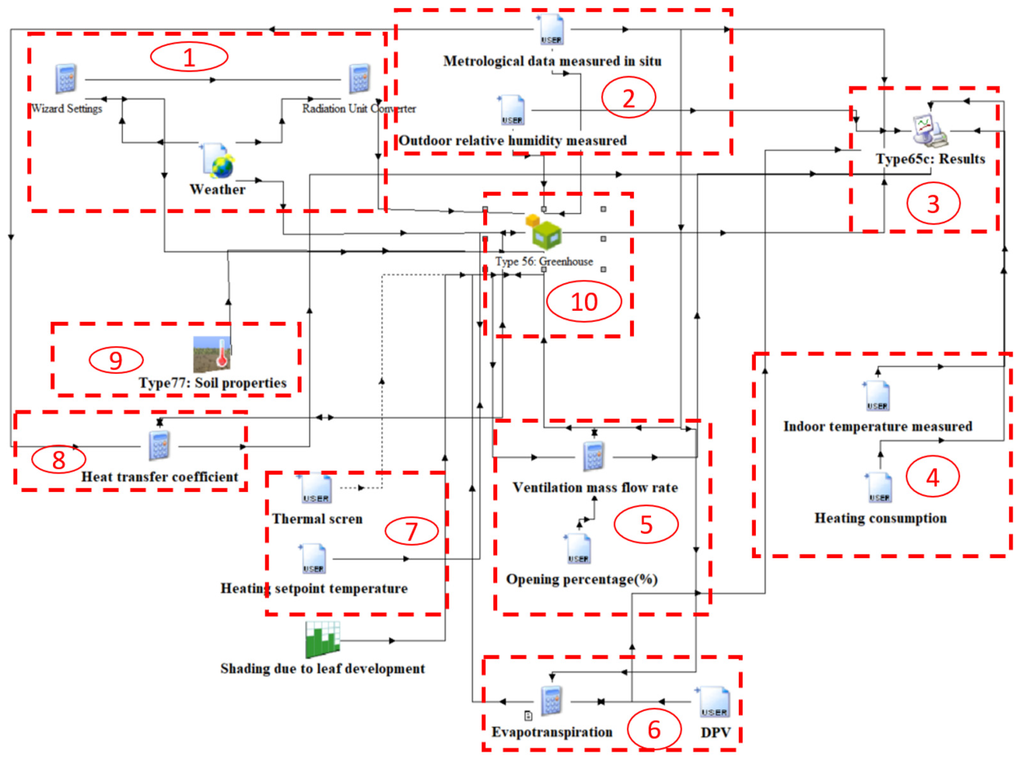
2.3. Simulation Model

2.3.1. Modeling Procedure

The first step of the modeling was to create a TRNSYS 3D building Multizone model file, in which the SketchUp 3D greenhouse drawing was imported. The volumes, the floor areas, the wall types, and the orientations of each surface of every zone were carefully respected.

Type56 of the TRNSYS software integrated modules for the calculation of thermal demands in heating and cooling, hygric needs, losses due to infiltration, and internal heat gains. A part of the electric consumption by LED lighting and equipment constituted free heat gains and slightly contributed to the reduction in the heating consumption. It was assumed that 30% of the electric consumption was converted into heat. This internal gain was nevertheless negligible compared with the global heating consumption of the CTIFL greenhouse. Figure 4 shows the TRNSYS scheme of the CTIFL greenhouse.

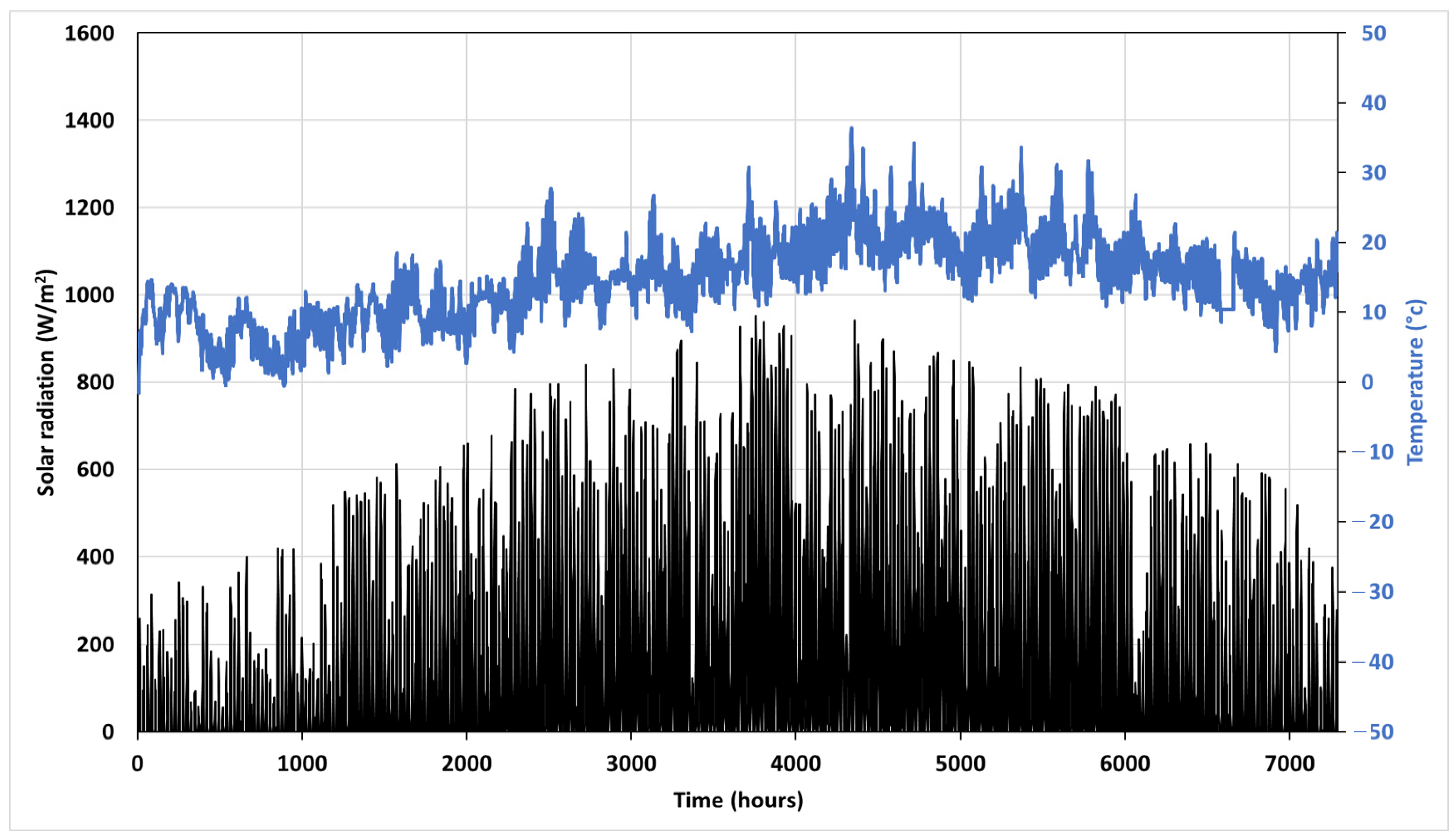
2.3.2. Weather Data File

The simulations were performed under the oceanic climatic conditions from the Meteonorm TRNSYS weather data file of Nantes and the experimental data measured on the site of CTIFL in Carquefou (at 20 km from Nantes’ meteorological station) over a period from 1 January 2015 at 00:00 until 31 October 2015 at 23:00 (Figure 5). This period corresponded to a complete period of cultivation, the end of the year being used for the cleaning and the preparation of the next year.

The TRNSYS environment had a database of TMY (Typical Meteorological Year) files that simulated typical years based on 30-year records for each site. These files took into account the usual colder or warmer periods of the year. The data used in these meteorological files included dry and humid air temperatures; air humidity; sky temperature; direct, diffuse, and total solar radiation; wind speed; and direction. Meteorological data were also collected by CTIFL on their site. A comparison of the two datasets showed a very strong similarity (

Table 5. Comparison of experimental and simulated monthly outdoor temperature and solar radiation.

Month	Mean Monthly External Temperature (°C)			Mean Monthly External Solar Radiation (W/m2)
	TRNSYS File	Experimental Data	Absolute Deviation	TRNSYS File	Experimental Data	Relative Deviation
January	7.9	5.2	2.7	41.8	42.6	−1.9%
February	6.5	5.8	0.6	74.0	79.1	−6.4%
March	10.2	8.0	2.3	119.4	118.8	0.5%
April	14.3	10.1	4.3	177.4	185.2	−4.2%
May	15.6	13.6	1.9	201.6	202.2	−0.3%
June	19.6	16.6	3.1	248.6	264.1	−5.9%
July	20.6	19.1	1.5	243.6	217.9	11.8%
August	20.8	18.5	2.3	211.3	191.0	10.6%
September	16.6	16.2	0.4	157.9	166.7	−5.3%
October	13.4	12.8	0.6	94.1	96.3	−2.3%

). The average absolute difference for temperatures was 1.97 K, and the average relative difference for relative humidity was −0.34%. This showed that the climate during the period of the measurements was close to that of a typical meteorological year. Some pieces of data from the TMY model were used to complete the experimental data because they were missing in the CTIFL file, namely, the decomposition of the solar radiation into direct and diffuse radiation shares, the sky temperature, the (angular) height of the sun, and the soil reflectance. The CTIFL meteorological data were taken in priority, completed with data from the TRNSYS TMY file.

3. Results and Discussion

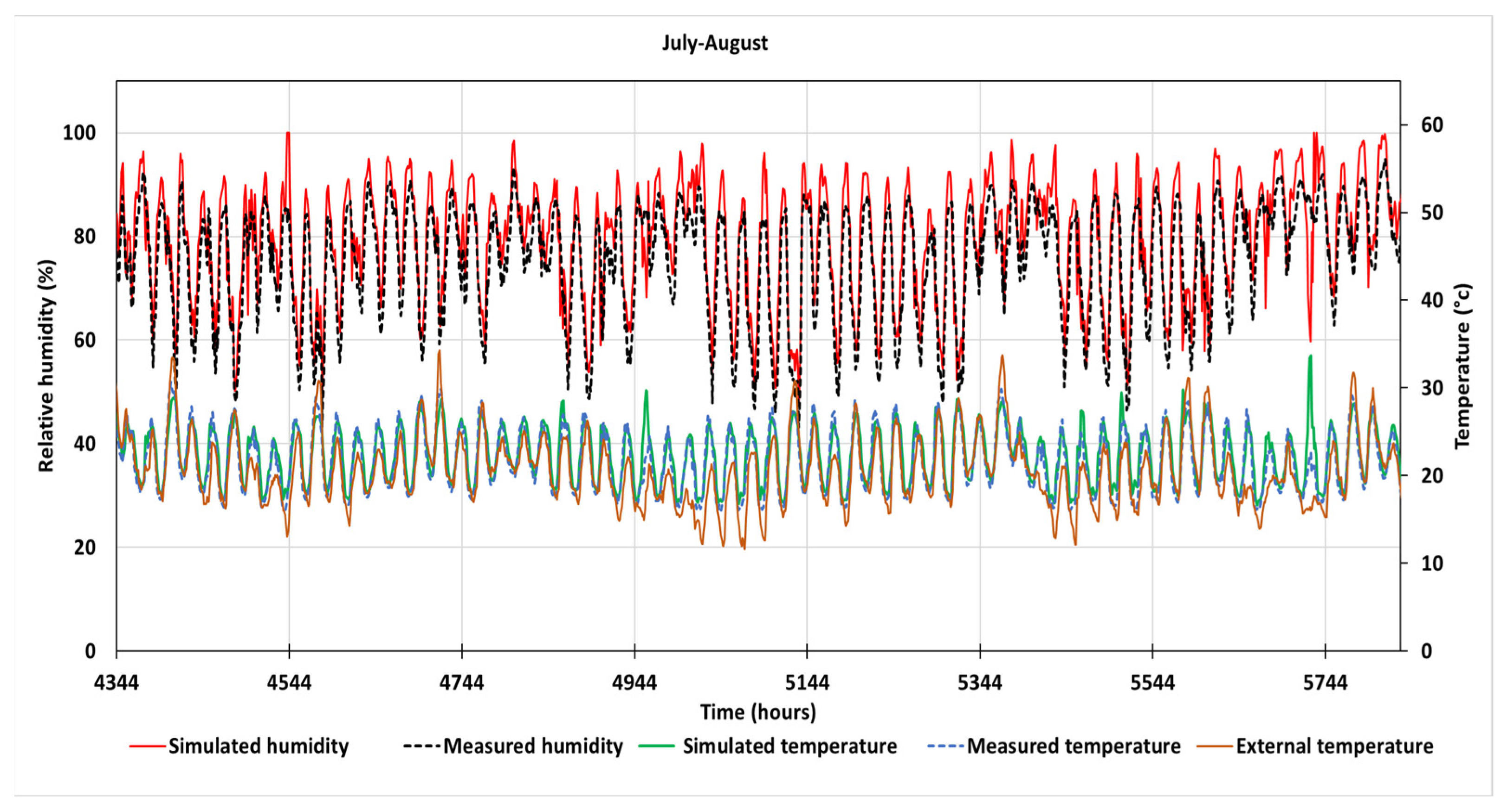
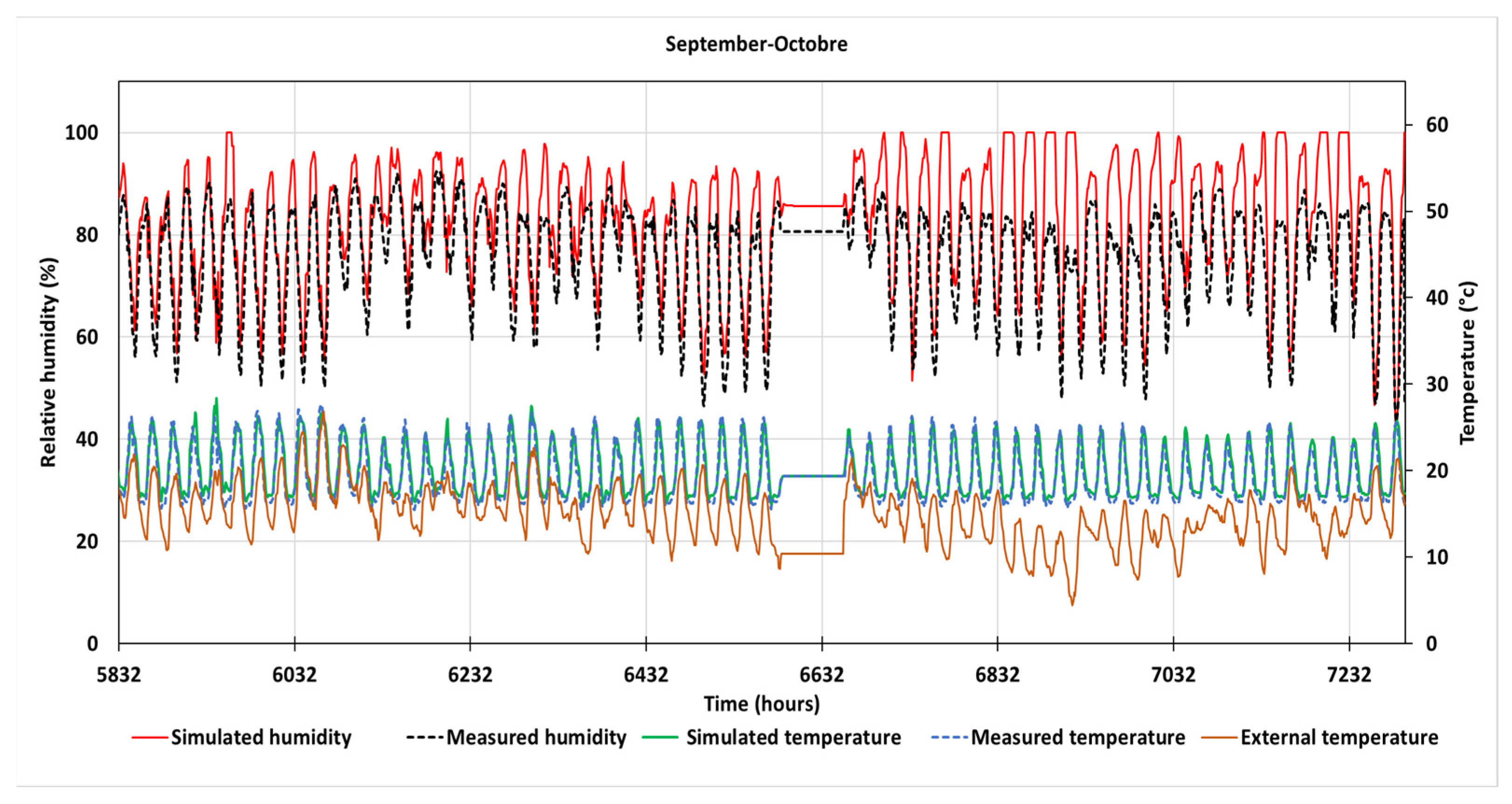
3.1. Model Validation by Comparison of Simulated and Experimental Results

3.1.1. Experimental Data

The CTIFL greenhouse was equipped by different systems of measurement and control in order to monitor the plants’ growth. The heating process was ensured using a ground rail pipe, a double vegetation pipe, and a polyethylene substrate pipe. An energy screen (Svensson XLS 10 Ultra Revolux) with a direct light transmission of 85% was installed at a height of 6.97 m from the ground floor. In addition, a screen (Svensoon XLS 35F Harmony Revolux) was used for shading with a direct light transmission of 65%. The two screens were driven by motor gearboxes (Ridder RW243). The ventilation was carried out by openings on the roof of the greenhouse: 72 main openings of 1.5 m × 1.4 m plus 12 openings on the sides of 0.675 m × 1.4 m. Two motor gearboxes (Ridder RW240) drove the support system. The software MultiMa (Ridder) was used to control the openings and the screens. The external climate data (temperature, humidity, wind velocity, and direction) were monitored using a weather station (Ridder). The indoor climate (air temperature and relative humidity) and vapor pressure deficit (VPD) were monitored during 10 months with a time step of 5 min. The main characteristics of sensors are summarized in

Table 6. Instruments used to monitor the greenhouse indoor climate.

	Sensor Type	Measuring Range	Uncertainty
Temperature	PT100	−10 to 50 °C	$\pm$0.1 °C
Relative humidity	HMP110	0 to 100%	$\pm$1.5%
VPD	Infra-red OPTRIS (OPTCTLT 15 CFCB8)	−50 °C to 975 °C	$\pm$1 °C

. For energy consumption monitoring, standard electric and gas counters were used. The outdoor and indoor solar radiations were measured using two digital pyranometers (Hukesflux SR05) with 95% as a measurement confidence level. The different Ridder modules were linked together using the Synopta interface to control the indoor climate, the lighting strategy, the CO₂ injection, and eventually the plants’ development.

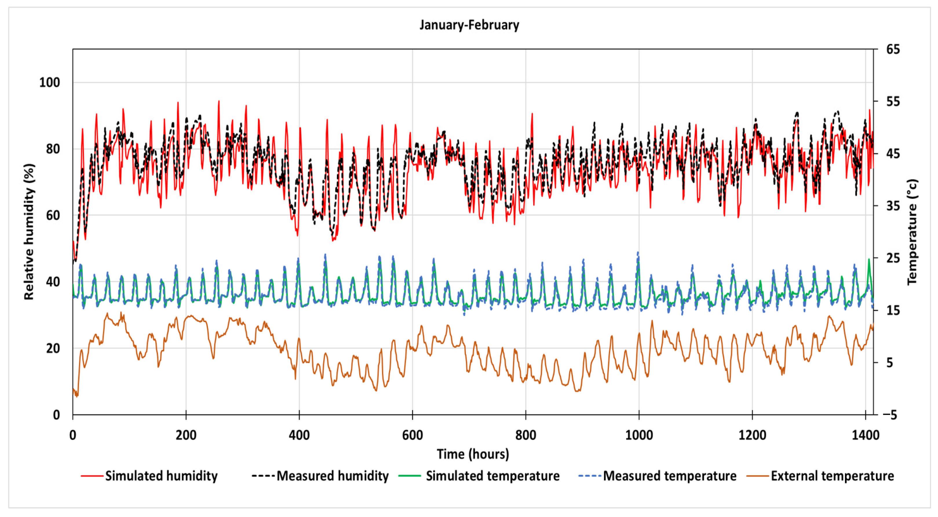
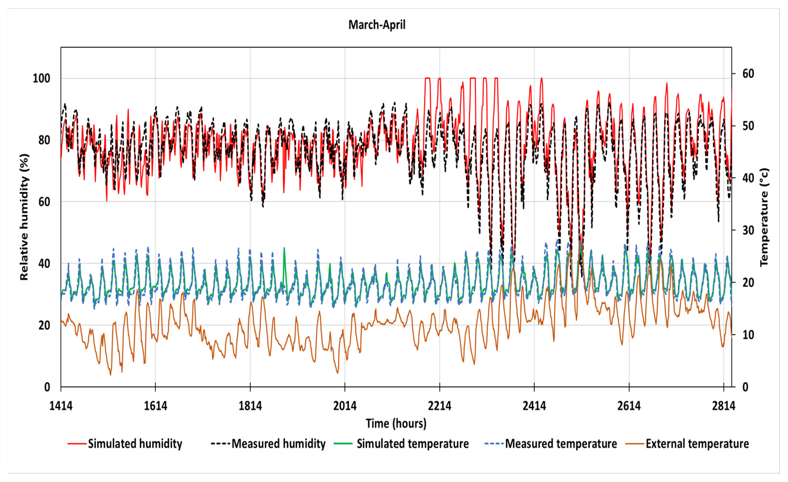
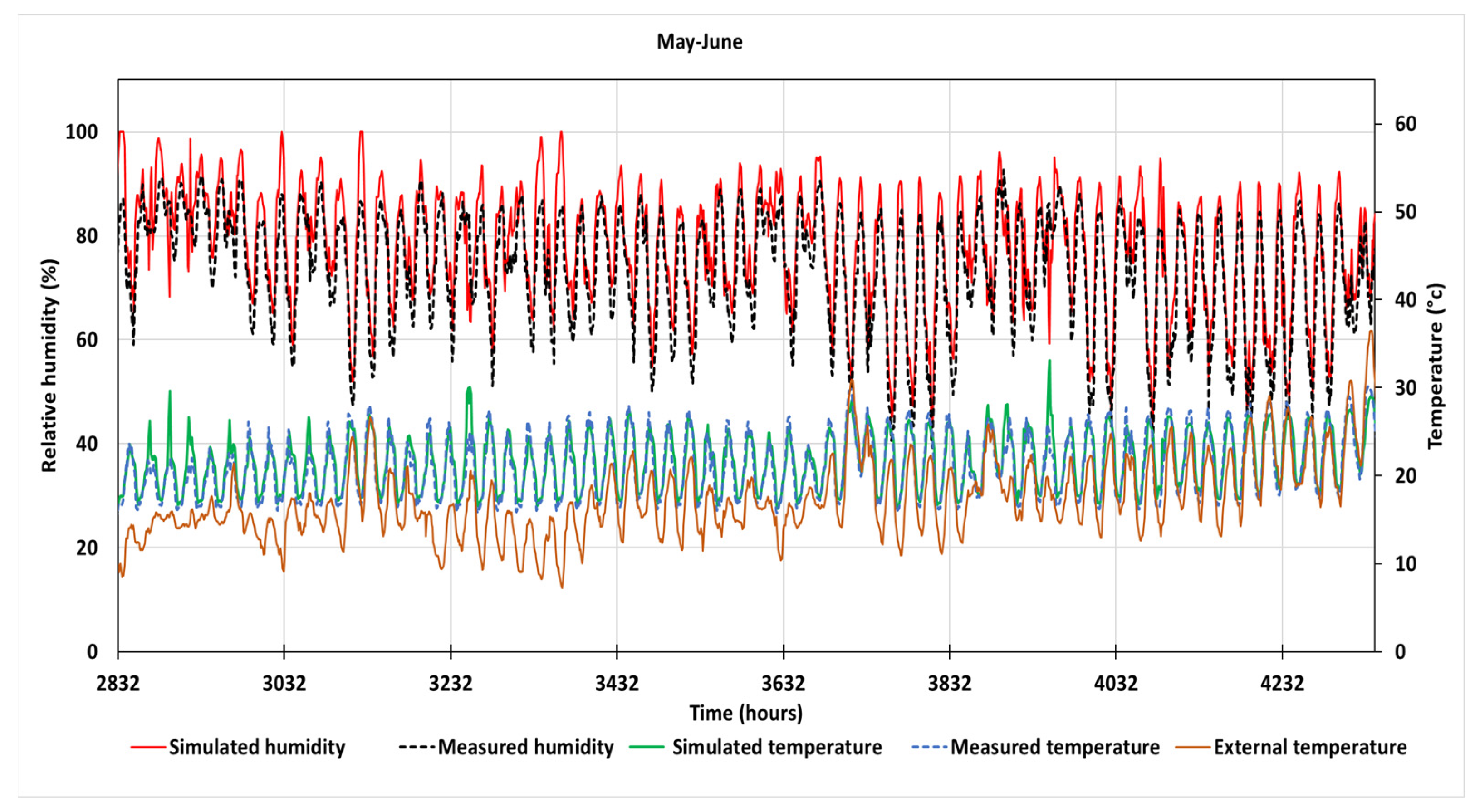
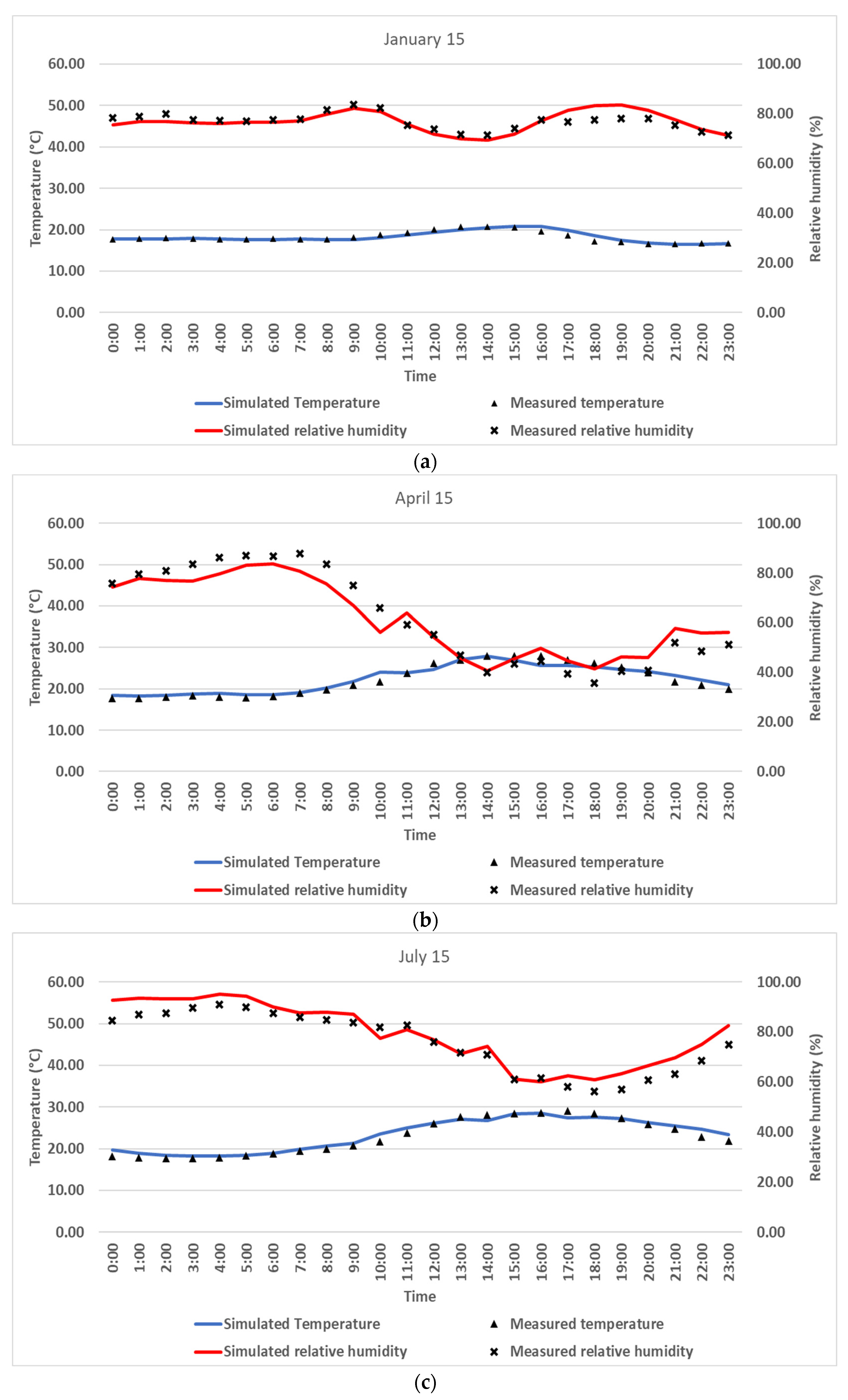
3.1.2. Model Validation

Figure 6, Figure 7, Figure 8, Figure 9 and Figure 10 show a comparison between the experimental and simulation results of two consecutive months. The air temperature inside the greenhouse calculated by the simulation was generally in good agreement with the experimental measurements. Nevertheless, the model overestimated the temperature by 5 K punctually at temperature peaks for a few days (7 days over the season). These peaks occurred when the solar irradiance was at its maximum. At these times of high solar radiation, a special manual action was performed on the real greenhouse to limit the temperature, such as a higher ventilation rate achieved by wide door openings. The indoor relative humidity variation calculated by the model slightly differed from the experimental data. The difference was attributed to the low accuracy of the camera used to measure the leaf area index (LAI) and the vapor pressure deficit (VPD) and to the high sensitivity of these parameters in Equation (5) calculating the evapotranspiration rate. The difference remained acceptable with respect to other studies that attempted to predict the relative humidity in greenhouses [1,49].

Table 7. Comparison of experimental and simulated monthly temperature and relative humidity.

Month	Mean Monthly Temperature (°C)			Mean Monthly Relative Humidity (%)
	Simulation Results	Experimental Data	Absolute Deviation (K)	Simulation Results	Experimental Data	Relative Deviation (%)
January	18.1	18.0	0.1	72.7	74.2	2%
February	18.0	17.7	0.3	75.0	77.1	3%
March	19.4	19.2	0.2	77,2	78.8	2%
April	20.5	20.3	0.2	79.5	73.7	8%
May	21.0	20.4	0.6	80,3	75.7	6%
June	22.3	22.0	0.3	74.4	70.3	6%
July	22.4	21.8	0.6	78.9	74.6	6%
August	22.3	21.6	0.7	79.7	75.7	5%
September	20.4	19.8	0.6	80.8	75.8	7%
October	19.6	19.1	0.5	84.5	75.7	12%

shows the monthly average indoor temperature and relative humidity and the monthly average absolute and relative differences between the simulated and experimental results. The monthly average values of the measured and calculated temperatures were very close. The average absolute deviation was generally lower than 0.7 K for the temperature, and the average relative deviation was generally lower than 8% for the relative humidity. In October, the interruption of the measurements due to a punctual failure of the acquisition system could explain the increase in the relative deviation between the measurement and prediction on the relative humidity, also visible in Figure 10. Apart from this particular period of October, and as specified above, the observed differences on relative humidity could be explained by the lack of precision of the method of measurement of VPD and of the exact leaf area and by the limits and high sensitivity of the empirical laws of evapotranspiration calculation.

In order to complete the validation and to give more credit to the model, the comparison of the simulated and experimental results was carried out for three days, one in winter, one in inter-seasons, and one in summer (Figure 11). Figure 11a–c show discrepancies between measured and simulated relative humidity. These errors came from the lack of acuteness of the model to exactly reproduce the variations due to the real indoor climate management system.

Table 8. Comparison of experimental and simulated temperature and relative humidity for three days (15 January, 15 April, and 15 July).

	Mean Temperature (°C)			Mean Relative Humidity (%)
	Simulation Results	Experimental Data	Absolute Deviation (K)	Simulation Results	Experimental Data	Relative Deviation (%)
15 January	18.2	18.2	0.0	76.8	76.9	0%
15 April	22.4	22.2	0.2	61.6	62.1	−1%
15 July	23.3	23.0	0.4	79.0	75.6	4%

shows the mean errors for temperature and humidity. The corresponding root mean square errors on each day were lower than 1.04 K for the temperature and lower than 5.38% for the relative humidity.

The energy consumption predicted by the TRNSYS simulation, for heating the CTIFL greenhouse between 1 January and 31 October, was 310 kWh·m⁻². The consumption measured experimentally was 300 kWh·m⁻², which corresponded to a relative difference of 3.5%. In the light of these results, the model was considered as validated to reproduce the hygrothermal behavior of the CTIFL greenhouse.

3.2. Parametric Study

The objectives of this section were to identify the shares of energy consumption due to the compensation of heat losses through the envelope, due to evapotranspiration and ventilation (1), and to evaluate the effects of changing the glazing type for a double-glazing in the roof (2), varying the thermal inertia of the ground (3) and suppressing the thermal buffer zone (4) and the thermal/shading screens (5).

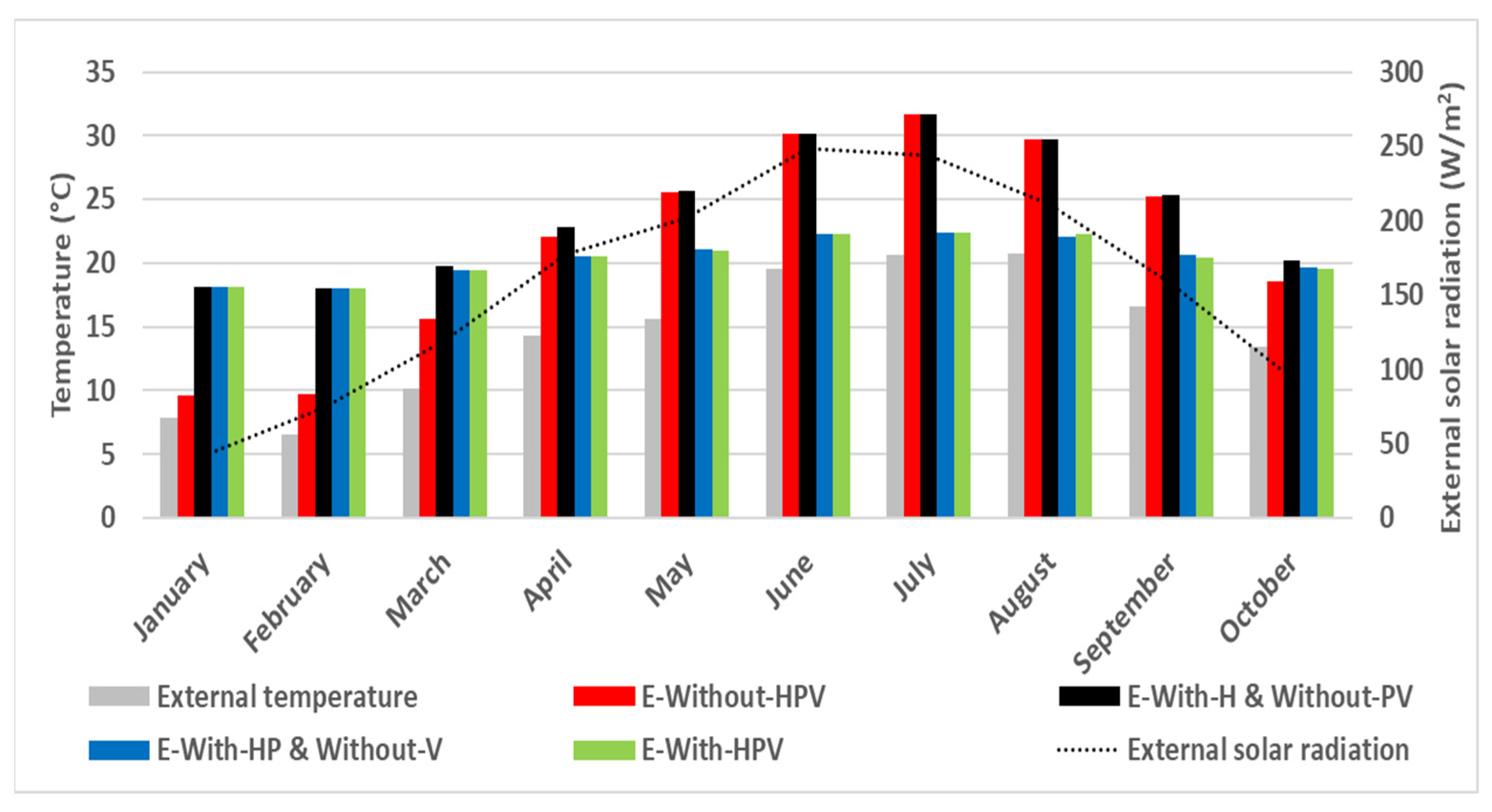
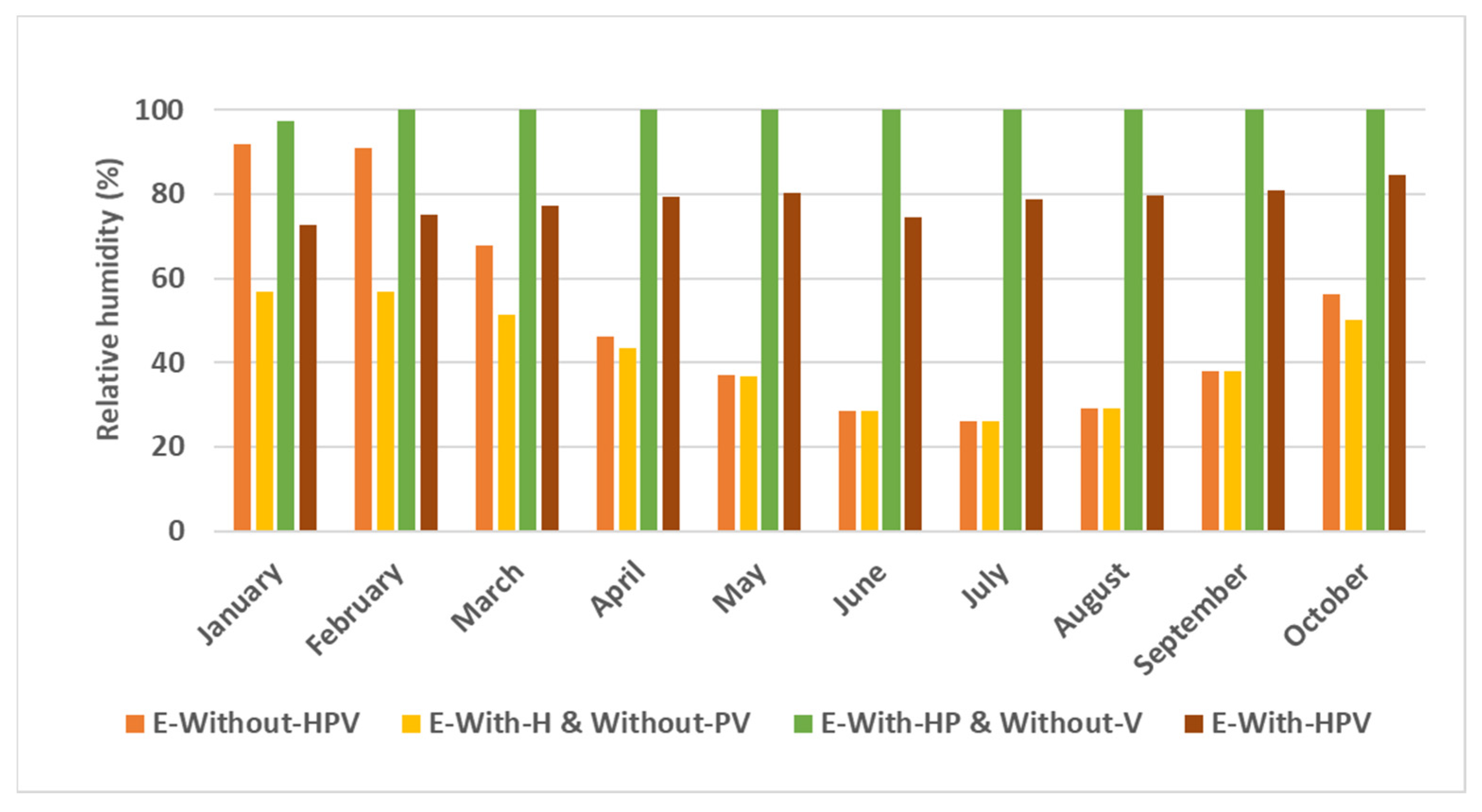
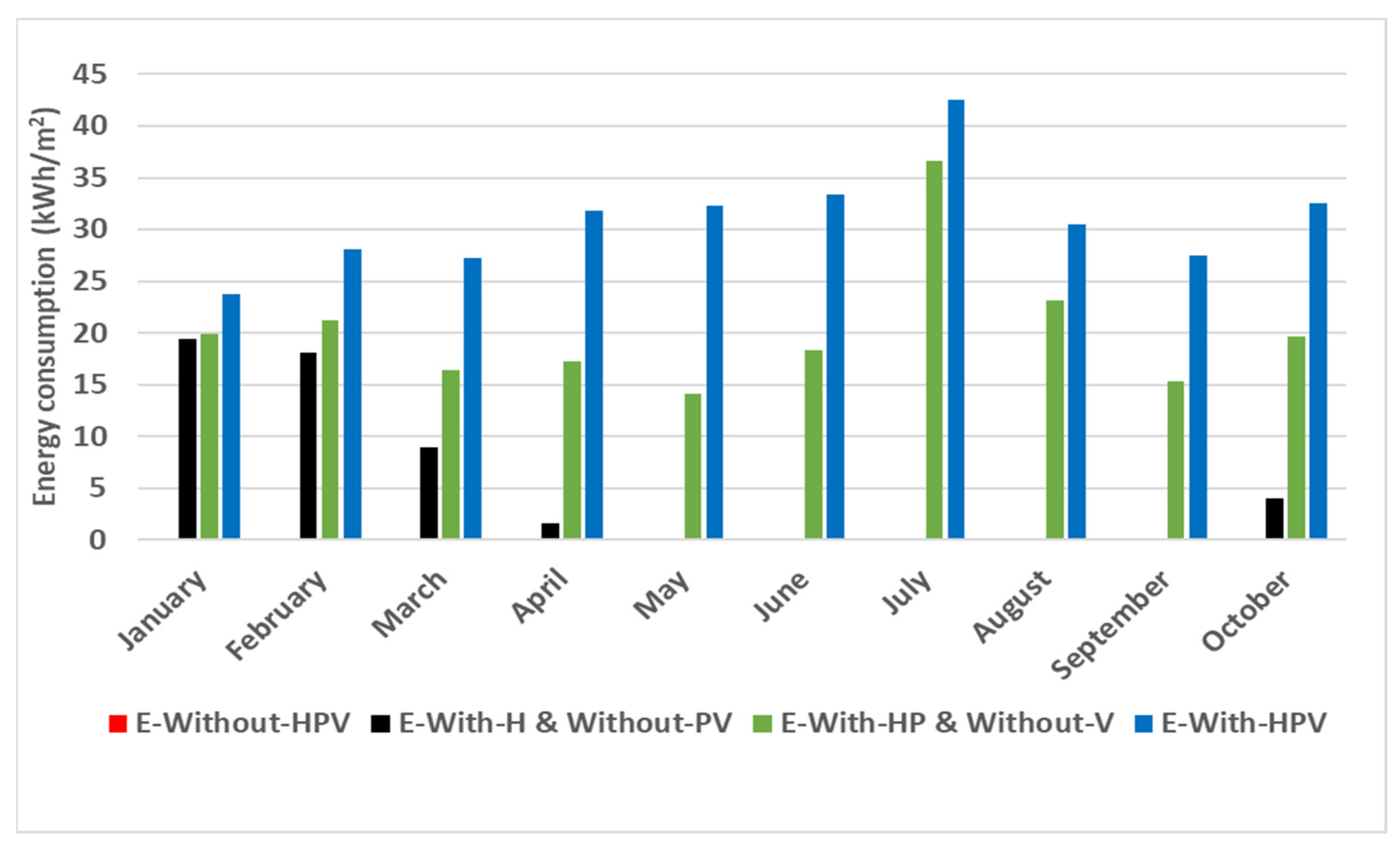
3.2.1. Identification of Different Contributions in Energy Consumption

Four simulations with different combinations of contributions to heating consumption were conducted. The contributions were combined as follows:

• Envelope in free evolution without heating, plants, and ventilation (E-Without-HPV);
• Envelope with heating to maintain real CTIFL annual air temperature variation, without plants and ventilation (E-With-H&Without-PV);
• Envelope with heating to maintain real CTIFL annual air temperature variation, with plants and without ventilation (E-With-HP&Without-V);
• Envelope with heating to maintain real CTIFL annual air temperature variation, with plants and ventilation (E-With-HPV).

Figure 12 and Figure 13 show the variations of monthly average temperature and relative humidity, respectively, for the four cases. When the greenhouse envelope was considered in free evolution (E-Without-HPV), the indoor air temperature was only influenced by the average external air temperature and solar radiation variations. The monthly average air temperature in the greenhouse was always warmer than the monthly average outside air, with a difference ranging from 2 to 12 K. The solar radiation captured by the greenhouse resulted in a temperature difference between the greenhouse and the outside, which exceeded 10 K during the summer. The heating system enabled increasing the indoor air temperature when necessary (E-With-H&Without-PV). The evapotranspiration of the tomato plants reduced the indoor temperature during the summer (E-With-HP&Without-V). However, the relative humidity stayed very high over the entire the year (in agreement with the results of Hou et al. [5]). The ventilation by the openings reduced relative humidity to an acceptable level around 80% (E-With-HPV).

Figure 14 shows the heating energy consumptions in the four considered scenarios to control the annual air temperature variation observed experimentally in the CTIFL greenhouse. In the scenario E-Without-HPV, the consumption was equal to zero. In the scenario E-With-H&Without-PV, the heat consumption compensated the heat losses through the envelope. The heating needs were zero from May to August, were low in April and October, and were high in January, February, and March. In the scenario E-With-HP&Without-V, the supplementary heat consumption relative to the former scenario was the evapotranspiration adiabatic cooling compensation due to the presence of tomato plants in the unventilated greenhouse. In the scenario E-With-HPV, the heating consumption increased compared with the E-With-HP&Without-V scenario because supplementary heating compensated the ambient air cooling due to the ventilation necessary to reach relative humidity levels in the greenhouse that were acceptable for plants.

Table 9. Contribution of different heat losses in the annual energy consumption.

	Energy Consumption (kWh·m−2)	Heat Loss Parts	Value (kWh·m−2)
E-With-H&Without-PV	56	Heat loss envelope compensation	56
E-With-HP&Without-V	211	Heat loss envelope compensation	56
		Heat loss evapotranspiration compensation	155
E-With-HPV	310	Heat loss envelope compensation	56
		Heat loss evapotranspiration compensation	155
		Heat loss ventilation compensation	99

summarizes the cumulated energy consumptions from 1 January until 31 October. It can be concluded that the heat compensation of the evapotranspiration phenomenon represented 50% of the total energy consumption. The heat losses due to ventilation and thermal transfer trough the envelope represented 32% and 18%, respectively.

3.2.2. Effect of Glazing Type

The effect of the glazing type was tested numerically. A simulation was run with a double glazing (4 mm air gap) on the roof instead of the simple glazing implemented in CTIFL. The U-value of the double glazing was 1.69 W·m⁻²·K⁻¹, and the g-value was 0.66. The energy consumption was reduced to 265 kWh·m⁻². There was a 14.5% reduction in the energy consumption compared with the base case (310 kWh·m⁻²). However, in spite of the increase in the thermal performance, the use of a double glazing reduced the transmitted solar radiation. In our example, the g-value decreased from 0.9 to 0.66. This would slow down the growth of the tomato plants. Moreover, the investment costs for double glazing would be much higher than those for simple glazing.

3.2.3. Effect of Thermal Inertia

Simulations were carried out with higher thicknesses of inert materials in the ground floor. The existing greenhouse had a floor area of 1037 m². A surface of only 72 m² was covered by a concrete slab. The rest was the original ground. A parametric study of the effect of thermal inertia was conducted by adding a concrete slab in the rest of the floor with variable slab thickness (0.25, 0.50, and 0.75 m). The maximum relative difference in energy consumption was lower than 5% (295 kWh·m⁻² instead of 310 kWh·m⁻²). This result could be explained by two reasons. First, the shading effect of the leaves stopped a part of the incident solar radiation on the floor surface. Second, the energy consumption due to the heat losses through the walls of the greenhouse represented only 18% of the total heating consumption (Table 9).

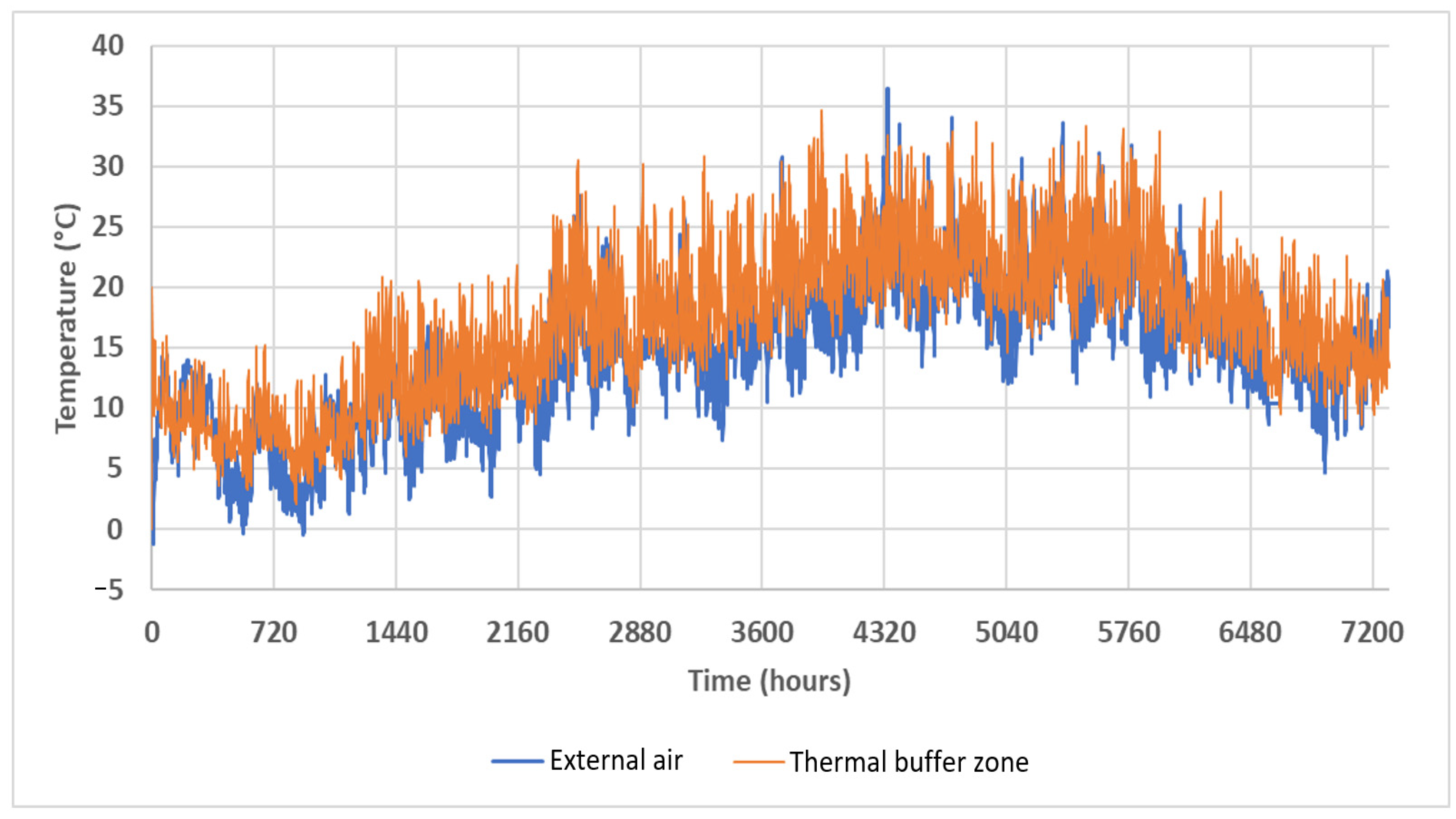
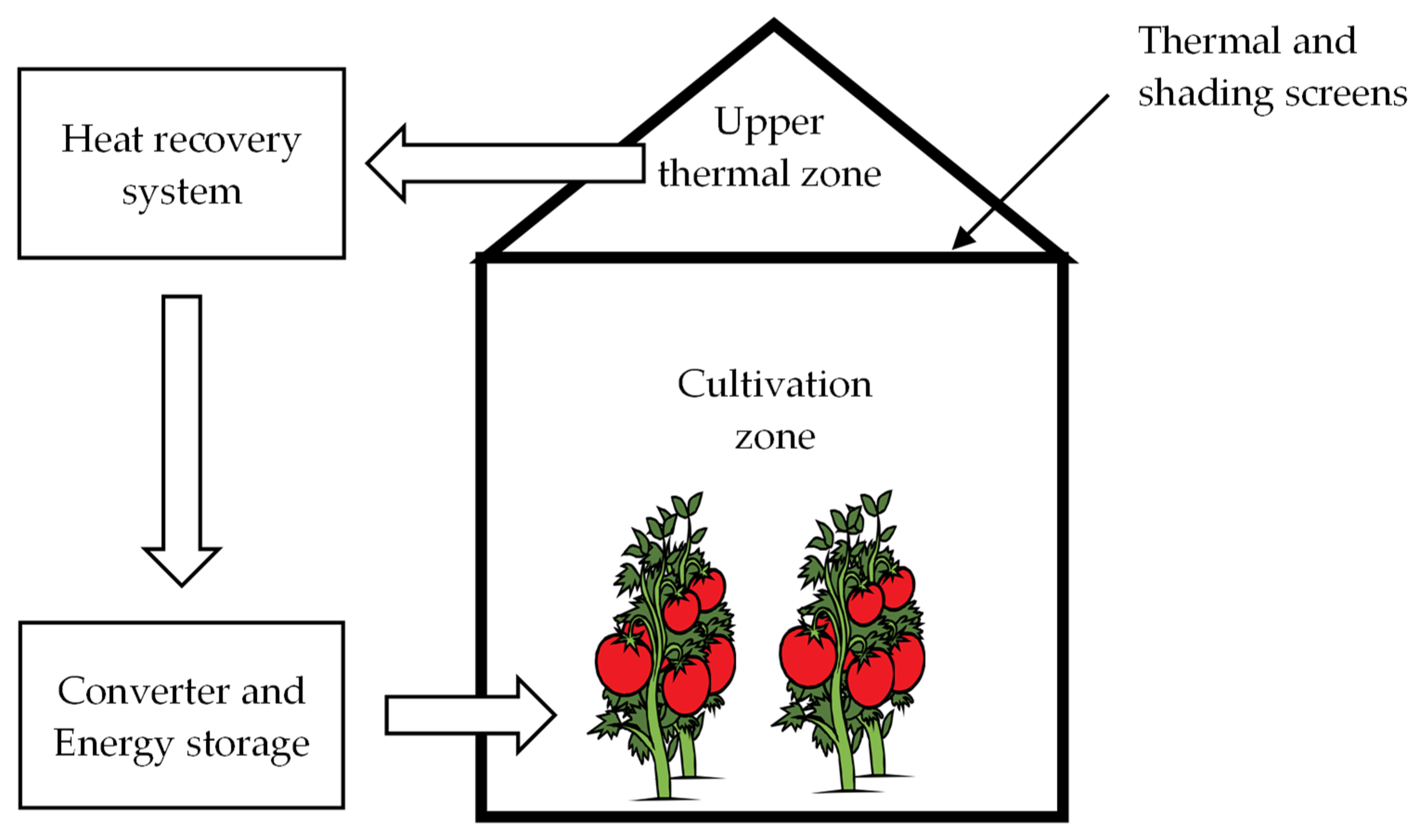
3.2.4. Effect of Thermal Buffer Zone

The thermal buffer zone was the area protected by a second peripheral glazing in the CTIFL greenhouse. It also had a practical role representing a covered circulation area for workers. As a thermal buffer zone, it reduced the heat losses through the vertical walls. Figure 15 shows the hourly variations of air temperatures outdoors (external air) and inside the thermal buffer zone. The air inside the thermal buffer zone was always hotter than the external one. The air temperature difference varied between 0 and 15 K. The absence of the thermal buffer zone would have put the vertical walls of the greenhouse in direct thermal contact with the outdoor air, leading to higher convective heat losses and higher energy consumptions. The simulation of the greenhouse without the thermal buffer zone produced an energy consumption equal to 600 kWh·m⁻², corresponding to an increase of about two-fold. In view of this significant thermal impact of the double-skin on greenhouse heat consumption, the concept of the thermal buffer zone should be generalized. In this configuration, the buffer zone represented 20% of the total greenhouse ground area. The dimensions of this zone should be optimized in new designs.

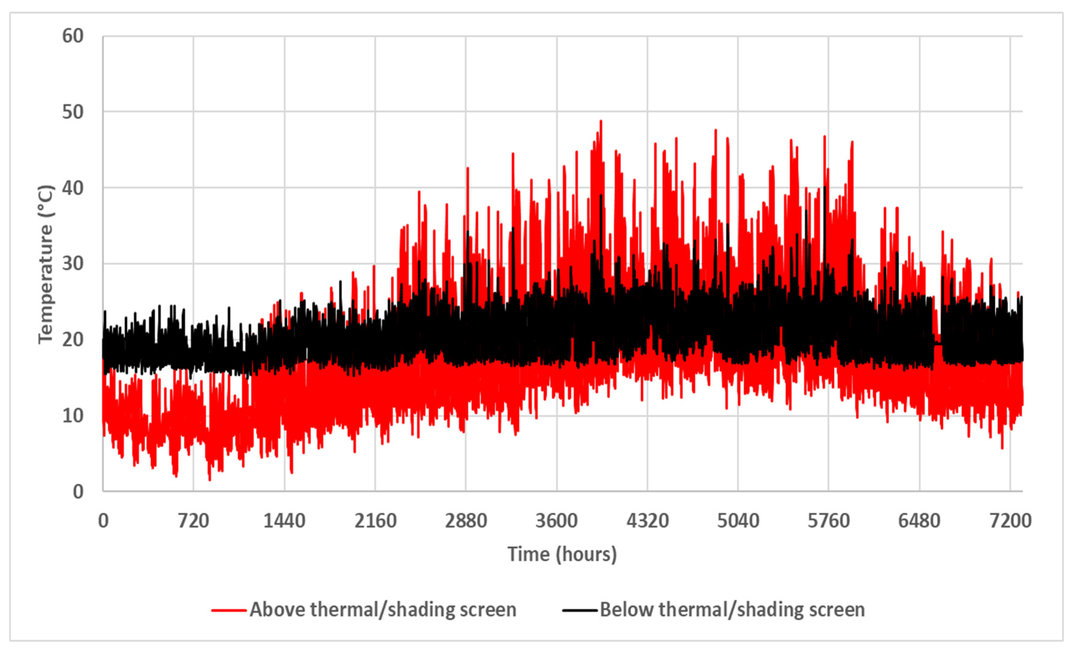
3.2.5. Effect of Thermal and Shading Screens

The objective of adding thermal and shading screens was to protect the plants against overheating during sunny days and to reduce heat losses during cold days [2,7,50]. Both screens were supposed to have the same thermal properties. Figure 16 illustrates the hourly variation of the air temperature above and below the screens. The temperature above the screens showed an important amplitude between day and night. Furthermore, situations of overheating were observed from April to September (from 2160 to 5760 h). The temperature reached 49 °C as a maximum. Regarding the energy consumptions, the thermal screen stopped the highest incident solar radiations and lowered evapotranspiration during sunny days. As a consequence, the energy consumption would increase from 310 to 440 kWh·m⁻² if the thermal screen was not used. The relative difference was about 45%, and it was practically the same as the one found in Rasheed et al. [7]. From Figure 16, it was judged possible to use the over-heated air to reduce the energy consumption during winter if it was stored in and recovered from a latent thermal energy storage as proposed in the review article of Ahamed et al. [51].

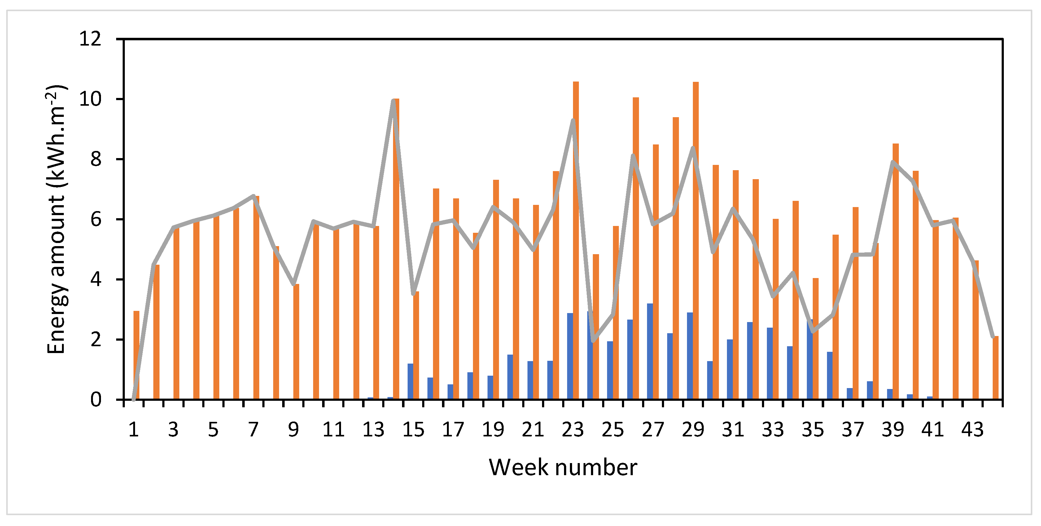
3.3. Heat Recovery Potential

Figure 15 shows that the thermal and shading screens separated two zones inside the greenhouse. The cultivation zone temperature and humidity were well controlled. During the summer, the zone above the thermal screen contained an energy amount that could be recovered (Figure 17).

As described in Section 2.1, the maximum temperature was fixed at 30 °C in the CTIFL greenhouse. The heat recovery potential was assumed to be equal to the cooling energy demand to maintain 30 °C inside the upper zone. The total heat recovery potential was 43 kWh·m⁻² over the year. When the upper zone was cooled at 30 °C during the summer, the windows were less open to ventilate the cultivation zone. The heating demand was reduced to 283 kWh·m⁻², corresponding to a non-negligible 9% decrease. If the annual heat recovery were to be stored, the chosen technology would be a long storage system such as the conversion into hydrogen. However, it is very complicated to convert low-grade heat into another type of energy. Electricity could be produced by an ORC with a low efficiency. Converting heat to electricity could enable the employment of any storage system (PHES, PTES, CAES, LAES…). The simplest heat recovery system would be a heating coil to heat water. The hot water would be stored in a high-capacity stratified reservoir for reuse during the next days. To study this option, the heat recovery potential could be evaluated every week. Figure 18 shows that it starts at week number 15, which corresponds to the end of April. The heat recovered during one week in the upper zone could contribute to decrease the heating energy consumption during the next week. Applying this assumption, the energy consumption was reduced to the gray line in Figure 18. The total energy consumption would be decreased by 24% to 237 kWh·m⁻² if the recovery and storage system were perfect.

4. Conclusions

The feasibility of the construction of a reliable model over a full cultivation season of a greenhouse for tomato cultivation using TRNSYS software was demonstrated in this article. The limitation of the model concerns its lack of acuity regarding convective movements and temperature stratification. TRNSYS could model these phenomena if more thermal zones were created vertically. However, no such measurement was available from the CTIFL greenhouse for validation, and this limitation did not prevent the correct calculation of the indoor temperature, indoor humidity, and energy consumption.

The CTIFL experimental semi-closed greenhouse in Carquefou near Nantes, France, was modeled, and the model was validated by comparison with experimental data collected on site. The model allowed the prediction of the annual heating consumption with an error of 3.5%. The temporal variations of the indoor air temperature and relative humidity were satisfactory, and the deviations observed on the prediction of the relative humidity were related to the limits of the leaf area measurement technique that weakened the empirical evapotranspiration model. The parametric study concluded that some variables were found critical because of their high influence on the results:

• The properties of glazed surfaces;
• The presence of a thermal buffer zone;
• The heat exchange by convection with the outdoor air;
• The ventilation rate;
• The evapotranspiration of plants.

Other parameters were identified as not influential because of their low contribution to the thermal behavior of the greenhouse with respect to influential variables:

• The inert mass inside the greenhouse;
• The internal lighting gains, LED technology being assumed;
• The internal electric gains due to equipment.

The energy consumption ratio was 310 kWh·m⁻², 18% for compensating heat losses through the envelope, 50% for evapotranspiration compensation, and 32% for ventilation heat losses. The evapotranspiration and ventilation contributions to the energy consumption could be reduced by changing from a semi-closed to a fully closed greenhouse and implementing a dehumidification system. The heat recovery potential was very high in greenhouses. Up to 24% energy savings could be achieved by storing and then recovering subsequently the excess heat contained in the air of the upper zone of the greenhouse, over the thermal screen. The possible systems for a week are CAES, LAES, PTES, or more simply thermal storage in a stratified and well-insulated reservoir. Hydrogen or other synthetized gas could be a solution for longer storage.

In the future, the greenhouse model will be improved and implemented with submodels of new technologies aiming toward energy consumption minimization. Only the heat recovery potential was assessed in this study. Energy storage systems will be investigated and compared. The most interesting solutions are intended to be tested in experimental greenhouses to confirm their efficiency. As the weather can influence the choice of certain systems, other climatic conditions will also be applied to the model. Finally, the model will be extended to other types and dimensions of greenhouses.

References

1. Sanchez, E.A.; Retureta, G.L.; Flores, E.P.; Velazquez, A.L. Evaluation of thermal behavior for an asymmetric greenhouse by means of dynamic simulations. Dyna-Colomb. 2014, 81, 152–159. [Google Scholar] [CrossRef]
2. Altes-Buch, Q.; Quoilin, S.; Lemort, V. A modeling framework for the integration of electrical and thermal energy systems in greenhouses. Build. Simul. 2022, 15, 779–797. [Google Scholar] [CrossRef]
3. Yohannes, T.; Fath, H. Novel agriculture greenhouse that grows its water and power: Thermal analysis. In Proceedings of the 24th Canadian Congress of Applied Mechanics (CANCAM 2013), Saskatoon, SK, Canada, 2–6 June 2013. [Google Scholar]
4. Mashonjowa, E.; Ronsse, F.; Milford, J.R.; Pieters, J. Modelling the thermal performance of a naturally ventilated greenhouse in Zimbabwe using a dynamic greenhouse climate model. Sol. Energy 2013, 91, 381–393. [Google Scholar] [CrossRef]
5. Hou, Y.; Li, A.; Li, Y. Analysis of microclimate characteristics in solar greenhouses under natural ventilation. Build. Simul. 2021, 14, 1811–1821. [Google Scholar] [CrossRef]
6. Klein, S.A. TRNSYS 18: A Transient System Simulation Program; Solar Energy Laboratory, University of Wisconsin: Madison, WI, USA, 2017; Available online: http://sel.me.wisc.edu/trnsys (accessed on 3 October 2022).
7. Rasheed, A.; Kwak, C.S.; Kim, H.T.; Lee, H.W. Building Energy and Simulation Model for Analysing Energy Saving Options of Multi-Span Greenhouses. Appl. Sci. 2020, 10, 6884. [Google Scholar] [CrossRef]
8. Rasheed, A.; Na, W.H.; Lee, J.W.; Kim, H.T.; Lee, H.W. Optimisation of Greenhouse Thermal Screens for Maximized Energy Conservation. Energies 2019, 12, 3592. [Google Scholar] [CrossRef]
9. Patil, R.; Atre, U.; Nicklas, M.; Bailey, G.; Power, G. An Integrated Sustainable Food Production and Renewable Energy System with Solar & Biomass CHP; American Solar Energy Society: Austin, TX, USA, 2013. [Google Scholar]
10. Chargui, R.; Sammouda, H.; Farhat, A. Geothermal heat pump in heating mode: Modeling and simulation on TRNSYS. Int. J. Refrig. 2012, 35, 1824–1832. [Google Scholar] [CrossRef]
11. Candy, S.; Moore, G.; Freere, P. Design and modeling of a greenhouse for a remote region in Nepal. Procedia Eng. 2012, 49, 152–160. [Google Scholar] [CrossRef]
12. Banakar, A.; Montazeri, M.; Ghobadian, B.; Pasdarshahri, H.; Kamrani, F. Energy analysis and assessing heating and cooling demands of closed greenhouse in Iran. Therm. Sci. Eng. Prog. 2021, 25, 101042. [Google Scholar] [CrossRef]
13. Chahidi, L.O.; Fossa, M.; Priarone, A.; Mechaqrane, A. Greenhouse cultivation in Mediterranean climate: Dynamic energy analysis and experimental validation. Therm. Sci. Eng. Prog. 2021, 26, 101102. [Google Scholar] [CrossRef]
14. Rodríguez, F.; Yebra, L.J.; Berenguel, M.; Dormido, S. Modelling and simulation of greenhouse climate using Dymola. In IFAC Proceedings Volumes (IFAC-PapersOnline); IFAC Secretariat: Laxenburg, Austria, 2002; pp. 79–84. [Google Scholar]
15. Costantino, A.; Comba, L.; Sicardi, G.; Bariani, M.; Fabrizio, E. Energy performance and climate control in mechanically ventilated greenhouses: A dynamic modelling-based assessment and investigation. Appl. Energy 2021, 288, 116583. [Google Scholar] [CrossRef]
16. Taki, M.; Ajabshirchi, Y.; Faramarz Ranjbar, S.; Rohani, A.; Matloobi, M. Modeling and experimental validation of heat transfer and energy consumption in an innovative greenhouse structure. Inf. Process. Agric. 2016, 3, 157–174. [Google Scholar] [CrossRef]
17. van Beveren, P.J.M.; Bontsema, J.; van Straten, G.; van Henten, E.J. Minimal heating and cooling in a modern rose greenhouse. IFAC Proc. Vol. 2013, 46, 282–287. [Google Scholar] [CrossRef]
18. Esen, M.; Yuksel, T. Experimental evaluation of using various renewable energy sources for heating a greenhouse. Energy Build. 2013, 65, 340–351. [Google Scholar] [CrossRef]
19. Hepbasli, A. Low exergy modelling and performance analysis of greenhouses coupled to closed earth-to-air heat exchangers (EAHEs). Energy Build. 2013, 64, 224–230. [Google Scholar] [CrossRef]
20. Kumar, K.S.; Madan, K.; Jha, K.N.; Tiwari, A.P. Singh, Modeling and evaluation of greenhouse for floriculture in subtropics. Energy Build. 2010, 42, 1075–1083. [Google Scholar] [CrossRef]
21. Berroug, F.; Lakhal, E.K.; El Omari, M.; Faraji, M.; El Qarnia, H. Thermal performance of a greenhouse with a phase change material north wall. Energy Build. 2011, 43, 3027–3035. [Google Scholar] [CrossRef]
22. Mobtaker, H.G.; Ajabshirchi, Y.; Ranjbar, S.F.; Matloobi, M. Simulation of thermal performance of solar greenhouse in north-west of Iran: An experimental validation. Renew. Energy 2019, 135, 88–97. [Google Scholar] [CrossRef]
23. Byrne, P.; Lalanne, P. Parametric study of a long-duration energy storage using pumped-hydro and carbon dioxide transcritical cycles. Energies 2021, 14, 4401. [Google Scholar] [CrossRef]
24. Rahman, M.M.; Gemechu, E.; Oni, A.O.; Kumar, A. The development of a techno-economic model for the assessment of the cost of flywheel energy storage systems for utility-scale stationary applications. Sustain. Energy Technol. Assess. 2021, 47, 101382. [Google Scholar] [CrossRef]
25. Barnhart, C.J.; Benson, S.M. On the importance of reducing the energetic and material demands of electrical energy storage. Energy Environ. Sci. 2013, 6, 1083–1092. [Google Scholar] [CrossRef]
26. Odukomaiya, A.; Abu-Heiba, A.; Gluesenkamp, K.R.; Abdelaziz, O.; Jackson, R.K.; Daniel, C.; Graham, S.; Momen, A.M. Thermal analysis of near-isothermal compressed gas energy storage system. Appl. Energy 2016, 179, 948–960. [Google Scholar] [CrossRef]
27. Hunt, J.D.; Zakeri, B.; Lopes, R.; Barbosa, P.S.F.; Nascimento, A.; De Castro, N.J.; Brandão, R.; Smith Schneider, P.; Wada, Y. Existing and new arrangements of pumped-hydro storage plants. Renew. Sustain. Energy Rev. 2020, 129, 109914. [Google Scholar] [CrossRef]
28. Cavazzini, G.; Houdeline, J.B.; Pavesi, G.; Teller, O.; Ardizzon, G. Unstable behaviour of pump-turbines and its effects on power regulation capacity of pumped-hydro energy storage plants. Renew. Sustain. Energy Rev. 2018, 94, 399–409. [Google Scholar] [CrossRef]
29. Pujades, E.; Willems, T.; Bodeux, S.; Orban, P.; Dassargues, A. Underground pumped storage hydroelectricity using abandoned works (deep mines or open pits) and the impact on groundwater flow. Hydrogeol. J. 2016, 24, 1531–1546. [Google Scholar] [CrossRef]
30. Connolly, D.; Lund, H.; Finn, P.; Mathiesen, B.V.; Leahy, M. Practical operation strategies for pumped hydroelectric energy storage (PHES) utilising electricity price arbitrage. Energy Policy 2011, 39, 4189–4196. [Google Scholar] [CrossRef]
31. Olabi, A.G.; Wilberforce, T.; Ramadan, M.; Abdelkareem, M.A.; Alami, A.H. Compressed air energy storage systems: Components and operating parameters—A review. J. Energy Storage 2021, 34, 102000. [Google Scholar] [CrossRef]
32. Tallini, A.; Vallati, A.; Cedola, L. Applications of micro-CAES systems: Energy and economic Analysis. Proceedings of the 70th Conference of the ATI Engineering Association. Energy Procedia 2015, 82, 797–804. [Google Scholar] [CrossRef]
33. Bi, J.; Jiang, T.; Chen, W.; Ma, X. Research on Storage Capacity of Compressed Air Pumped Hydro Energy Storage Equipment. Energy Power Eng. 2013, 5, 26–30. [Google Scholar] [CrossRef]
34. Dib, G.; Haberschill, P.; Rullière, R.; Perroit, Q.; Davies, S.; Revellin, R. Thermodynamic simulation of a micro advanced adiabatic compressed air energy storage for building application. Appl. Energy 2020, 260, 114248. [Google Scholar] [CrossRef]
35. Kandezi, M.S.; Naeenian, S.M.M. Investigation of an efficient and green system based on liquid air energy storage (LAES) for district cooling and peak shaving: Energy and exergy analyses. Sustain. Energy Technol. Assess. 2021, 47, 101396. [Google Scholar]
36. Georgiou, S.; Shah, N.; Markides, C.N. A thermo-economic analysis and comparison of pumped-thermal and liquid-air electricity storage systems. Appl. Energy 2018, 226, 1119–1133. [Google Scholar] [CrossRef]
37. Steinmann, W.D.; Bauer, D.; Jockenhöfer, H.; Johnson, M. Pumped thermal energy storage (PTES) as smart sector-coupling technology for heat and electricity. Energy 2019, 183, 185–190. [Google Scholar] [CrossRef]
38. Mercangöz, M.; Hemrle, J.; Kaufmann, L.; Z’Graggen, A.; Ohler, C. Electrothermal energy storage with transcritical CO2 cycles. Energy 2012, 45, 407–415. [Google Scholar] [CrossRef]
39. McTigue, J.D.; White, A.J.; Markides, C.N. Parametric studies and optimisation of pumped thermal electricity storage. Appl. Energy 2015, 137, 800–811. [Google Scholar] [CrossRef]
40. Siemens-Gamesa Electric Thermal Energy Storage. Available online: https://deepresource.wordpress.com/2019/06/17/siemens-gamesa-electric-thermal-energy-storage (accessed on 17 October 2020).
41. Hu, G.; Chen, C.; Lu, H.T.; Wu, Y.; Liu, C.; Tao, L.; Men, Y.; He, G.; Li, K.G. A review of technical advances, barriers, and solutions in the Power to Hydrogen (P2H) roadmap. Engineering 2020, 6, 1364–1380. [Google Scholar] [CrossRef]
42. Yazdanian, M.; Klems, J.H. Measurement of the exterior convective film coefficient for windows in low-rise buildings. ASHRAE Trans. 1993, 100 Pt 1, LBL-34717. [Google Scholar]
43. Hamer, P.J.C. Validation of a model used for irrigation control of a greenhouse crop. Acta Hortic. 1998, 458, 75–82. [Google Scholar] [CrossRef]
44. Boulard, T.; Jemaa, R. Greenhouse tomato crop transpiration model application to irrigation control. Acta Hortic. 1993, 335, 381–388. [Google Scholar] [CrossRef]
45. Jemaa, R.; Boulard, T.; Baille, A. Apport des modèles de transpiration d’une culture de tomate sous serre au pilotaghe de l’irrigation. Cah. Options Mediterr. 1999, 31, 203–214. [Google Scholar]
46. Medrano, E.; Lorenzo, P.; Sanchez-Guerrero, M.C.; Garcia, M.L.; Caparros, I.; Gimenez, M. Influence of an external greenhouse mobile shading on tomato crop transpiration. Acta Hortic. 2004, 659, 195–199. [Google Scholar] [CrossRef]
47. Vanthoor, B.H.E.; Stanghellini, C.; van Henten, E.J.; de Visser, P.H.B. A methodology for model-based green-house design: Part 1, a greenhouse climate model for a broad range of designs and climates. Biosyst. Eng. 2011, 110, 363–377. [Google Scholar] [CrossRef]
48. De Zwart, H.F. Analyzing Energy-Saving Options in Greenhouse Cultivation Using a Simulation Model; Land-Bouw Universitet te Wageningen: Wageningen, The Netherlands, 1996. [Google Scholar]
49. Gavilán, P.; Ruiz, N.; Lozano, D. Daily forecasting of reference and strawberry crop evapotranspiration in greenhouses in a Mediterranean climate based on solar radiation estimates. Agric. Water Manag. 2015, 159, 307–317. [Google Scholar] [CrossRef]
50. Rabiu, A.; Na, W.; Akpenpuun, T.D.; Rasheed, A.; Adesanya, M.A.; Ogunlowo, Q.O.; Kim, H.T.; Lee, H. Determination of overall heat transfer coefficient for greenhouse energy-saving screen using Trnsys and hotbox. Biosyst. Eng. 2022, 217, 88–101. [Google Scholar] [CrossRef]
51. Ahamed, M.S.; Guo, H.; Tanino, K. Energy saving techniques for reducing the heating cost of conventional greenhouses. Biosyst. Eng. 2019, 178, 9–33. [Google Scholar] [CrossRef]
Figure 1. A 3D model of the CTIFL greenhouse cultivation zone.
Cleantechnol 05 00058 g001
Figure 2. A 3D model of the thermal buffer zone that surrounds the greenhouse.
Cleantechnol 05 00058 g002
Figure 3. A 3D model of the CTIFL greenhouse with its thermal buffer zone.
Cleantechnol 05 00058 g003
Figure 4. Modeling scheme of the CTIFL greenhouse in the TRNSYS Studio. Block 1: Importation of solar radiation values from the weather data file and conversion to the appropriate unit for the TRNSYS calculation. Block 2: Importation of the metrological data from the CTIFL site. Block 3: Visualization of the results (simulation results + experimental data) and then exportation of the results in an Excel file for post-processing. Block 4: Importation of temperature and humidity measurements in the greenhouse and of the heating consumption to have an hourly comparison during the simulation. Block 5: Calculation of the air renewal rate from the opening rate of the openings measured at CTIFL (Equation (9)). Block 6: Calculation of the quantity of water in kg/h emitted by evapotranspiration from the plant to the greenhouse air according to the incident solar radiation and the plant/air water deficit measured experimentally (Equation (5)). Block 7: Linking the heating set point as an input to the greenhouse. The thermal screen position is linked to the greenhouse to control the solar input. Block 8: Calculation of the convection heat transfer coefficient between the glazing and the outside air. The coefficient is recalculated every hour using the difference between the temperature of the glass and the outside temperature and the hourly value of the wind speed. Block 9: Definition of the thermophysical properties of the soil in order to calculate the heat exchange between the greenhouse and the ground. Block 10: Type56 representing the greenhouse envelope. In this block, the thermophysical properties of the materials (Table 2), the thickness of the walls, and the type of glazing (Table 2) are defined. The heating set points, ventilation parameters, and evapotranspiration gain are linked to this block as model inputs.
Cleantechnol 05 00058 g004
Figure 5. Typical external air temperature and solar radiation.
Cleantechnol 05 00058 g005
Figure 6. Hourly variation of temperature and relative humidity in the greenhouse from 1 January to 28 February.
Cleantechnol 05 00058 g006
Figure 7. Hourly variation of temperature and relative humidity in the greenhouse from 1 March to 30 April.
Cleantechnol 05 00058 g007
Figure 8. Hourly variation of temperature and relative humidity in the greenhouse from 1 May to 30 June.
Cleantechnol 05 00058 g008
Figure 9. Hourly variation of temperature and relative humidity in the greenhouse from 1 July to 31 August.
Cleantechnol 05 00058 g009
Figure 10. Hourly variation of temperature and relative humidity in the greenhouse from 1 September to 31 October.
Cleantechnol 05 00058 g010
Figure 11. Comparison of experimental and simulated results of indoor temperature and humidity on (a) 15 January, (b) 15 April, and (c) 15 July.
Cleantechnol 05 00058 g011
Figure 12. Mean monthly average temperature inside the greenhouse for different combinations, for the external air temperature and external solar radiation.
Cleantechnol 05 00058 g012
Figure 13. Mean monthly average relative humidity inside the greenhouse for different combinations.
Cleantechnol 05 00058 g013
Figure 14. Monthly heating consumption for different combinations.
Cleantechnol 05 00058 g014
Figure 15. Hourly variations of temperatures of external air and thermal buffer zone.
Cleantechnol 05 00058 g015
Figure 16. Hourly variation of above and below thermal/shading screens air temperatures.
Cleantechnol 05 00058 g016
Figure 17. Strategy of heat recovery from the upper thermal zone.
Cleantechnol 05 00058 g017
Figure 18. Variation of heat recovery potential (blue bars) and heating energy consumption without (orange bars) and with heat recovery (gray line).
Cleantechnol 05 00058 g018