1. Introduction
Injecting CO
2 into deep saline aquifers (DSAs) has been proposed as one of the most viable means of tackling global warming [
1]. This is because the technology has developed sufficiently due to the experience gained from oil and gas exploration and waste disposal methodologies. Moreover, the DSAs offer more extensive storage potential than other geological formations, such as oil and gas fields or coal seams [
1]. Consequently, many studies have been conducted to assess their storage capacity and efficiency to safely sequester the injected gas [
2,
3,
4,
5,
6,
7,
8].
As discussed earlier in our previous works [
9,
10], CO
2 storage methodology in saline aquifers can be categorised into hydrodynamic and chemical mechanisms. The first one includes the structural and residual trapping of CO
2 within the aquifer pore space, while the second one comprises of the solubility and mineral trapping of CO
2.
Two important factors that should be considered while assessing the suitability of an aquifer for sequestering CO
2 are its capacity and injectivity. They should allow for the safer and cost-effective storage of large amounts of the disposed gas [
11]. Additionally, hydrostatic conditions play a crucial role in increasing the storage of saline aquifers because the higher pressure in deeper formations induces gas compression, resulting in more storage of CO
2 in a specific volume of the aquifer [
12,
13,
14]. In this regard, the integrity of the caprock with low permeability is an essential consideration because any existing faults or cracks in the aquifer rock will result in the injected gas escaping to the surface. Porosity and permeability of the formation have significant influence on the selection of the appropriate site for carbon storage because the higher permeability of a medium allows fluids to migrate easily through the better-connected pores away from the injection well, which subsequently magnifies the capacity and efficiency of the aquifer to store CO
2 [
15,
16,
17,
18].
Theoretically, the storage capacity of an aquifer is the substantial limit of CO
2 that can be admitted into it [
19,
20]. However, this limit is not practically achievable due to various geological factors and engineering barriers (e.g., pore connectivity, lack of geological data, economic feasibility, legal regulations and infrastructure benchmarks). Therefore, a term called effective storage capacity has been coined [
21,
22], which has been a subject of a number of studies using different calculation methods. These methods involve the use of volumetric and compressibility methods [
23,
24,
25], mathematical models [
26], dimensional analyses [
27], analytical investigations [
28] and numerical modelling [
29,
30] to assess the efficiency of geological formations to sequester CO
2. Most of these studies are theoretical or analytical in nature based on 2D models that seem to lack sufficient interests for practical employment. Detailed comparison studies have been conducted to evaluate the impact of a variety of approaches and methodologies on estimating CO
2 sequestration in geological formations [
20,
31,
32].
One basic estimation method, which is widely adopted, is the U.S. Department of Energy (US-DOE) method. As explained in detail by Goodman et al. [
33], the method assumes an infinitive boundary and defines the efficiency of an aquifer to store CO
2 by the pore volume that is available to be occupied by the injected gas. It determines the CO
2 mass storage capacity and efficiency for an aquifer as:
where
is the total cross-sectional area of the domain,
defines the gross thickness of the formation,
is the total porosity of the rock,
and
represent the density of the injected CO
2 and the storage efficiency of the aquifer, respectively.
An earlier approach, proposed by Zhou et al. [
23] predicts the pressure build-up history and the impact on the actual storage efficiency in response to the CO
2 injection process. The authors define the storage efficiency factor as the volumetric fraction of the sequestered CO
2 per unit volume of pores in the potential domain. In spite of achieving good agreement between the analytical results and the numerically predicted values, the authors state that this method is not suitable for geological formations of low permeability that lead to lower injectivity, and creates more non-uniformity in the pressure build-up within the simulated domain. This is due to many simplifications and assumptions in the analytical solutions in their research work.
Another method, developed by Szulczewski [
34], considers both the residual and solubility trapping mechanisms in addition to the CO
2 migration capacity. The method is applicable to both open-boundary and pressure-limited systems. Additionally, this method counts the net thickness of the aquifer to calculate the pore volume instead of the gross thickness in heterogeneous domains. This is because most of the injected CO
2 targets the high-porosity layers, such as sandstone or carbonate rocks, rather than any intermingled layers of shale or clay that store negligible amounts of the injected gas.
For open-boundary systems, the total mass of CO
2 (
stored in an aquifer can be determined by [
34]:
where
is the density of CO
2 at prevailing temperature and pressure,
is the total length of the aquifer,
is the width of the well,
is the net thickness of the aquifer
is the porosity of the rock,
is the connate water saturation and
is the storage efficiency factor.
If the aquifer is classified as a pressure-limited system, the CO
2 mass is calculated as follows [
34]:
where
is the permeability of the aquifer,
is the compressibility,
is the temperature,
is the brine viscosity,
is the fracture pressure of the rock,
is the hydrostatic pressure,
is the average density of brine,
is the gravitational acceleration,
is the depth to the top of the aquifer and
represents the maximum dimensionless pressure in the system which needs to be determined numerically, solving a different set of partial differential equations (PDEs) for the pressure-limited flow system [
34].
Several techniques can be used to increase the capacity and efficiency of CO2 sequestration in saline aquifers that will consequently support the efforts by the Intergovernmental Panel on Climate Change (IPCC) to incite policy makers with the importance of deploying carbon capture and sequestration (CCS) as one of the cost effective technologies for confronting climate change and global warming concerns.
Geological formation capacity can be increased by improving the injectivity through increasing the injection mass flow rate or pressure to compensate the loss of permeability due to salt precipitation in the well vicinity. Furthermore, injecting into adjacent layers with high permeability helps with attenuating pressure build-up and, consequently, higher injection rates can be employed [
35,
36].
Using horizontal injection wells instead of vertical ones is one of the methods implemented to increase the injectivity and capacity of aquifers because it helps to diminish the pressure-build-up peaks around the injection well and spread pressure uniformly within the domain. Deploying this technique requires the determination of the minimum length of the horizontal well that is dependent on the effective radius of pressure disturbance around the vertical injection well [
37,
38,
39,
40].
It has been evidenced that the solubility of CO
2 into brine can be accelerated by injecting slugs of fresh brine on top of the storage formation during and after CO
2 injection. This can increase CO
2 dissolution by more than 40% within a period of 200 years, which reduces the risk of CO
2 leakage in long-term sequestration, according to the study by Hassanzadeh et al. [
41]. The study also investigated further factors that have significant impact on increasing the storage efficiency in saline aquifers, including optimizing the rate of the injected brine and transporting the injected and existing fluids within the reservoir in addition to the effect of aquifer properties, such as thickness, vertical anisotropy and layers of heterogeneity included within the media.
In their work, De Silva and Ranjith [
39] concluded that, while using horizontal injection wells in the absence of chase brine injection improves the storage of aquifers, vertical injection wells with chase brine injection performs better storage efficiency. However, the authors suggest that the injection process should be carried out over the whole thickness of the aquifer to maximize the storage capacity. In contrast, Khudaida and Das [
9] observed that injecting CO
2 into the lower section of a reservoir enhances the solubility trapping mechanism and subsequently increases the storage efficiency.
Introducing hydraulic fractures in formation rock can improve the injectivity by increasing the effective permeability of the aquifer, which facilitates migration and, consequently, preserves more contact between the injected CO
2 and the existing brine, in addition to preventing any pressure build-up within the aquifer. However, this technique needs a detailed characterization of the formation and has to be implemented with extra care to avoid causing any gas leakage [
38].
Keeping the above discussions in mind, this work aims to provide further understanding on how to assess the feasibility of a potential storage site by investigating the behaviour and migration of CO2-brine as a two-phase flow system in porous geological formations under various injection conditions and scenarios. It also demonstrates the effects of various site characteristics, such as heterogeneity and anisotropy, on the injectivity and safe storage of the injected CO2. To aid the above, the capillary pressure relationships for CO2-brine as a two-phase flow is also studied. It is envisaged that the results will address the applicability of different injection techniques in terms of orientation and continuity to enhance the capacity and efficiency of sequestering CO2 in geological formations.
2. Modelling Setup
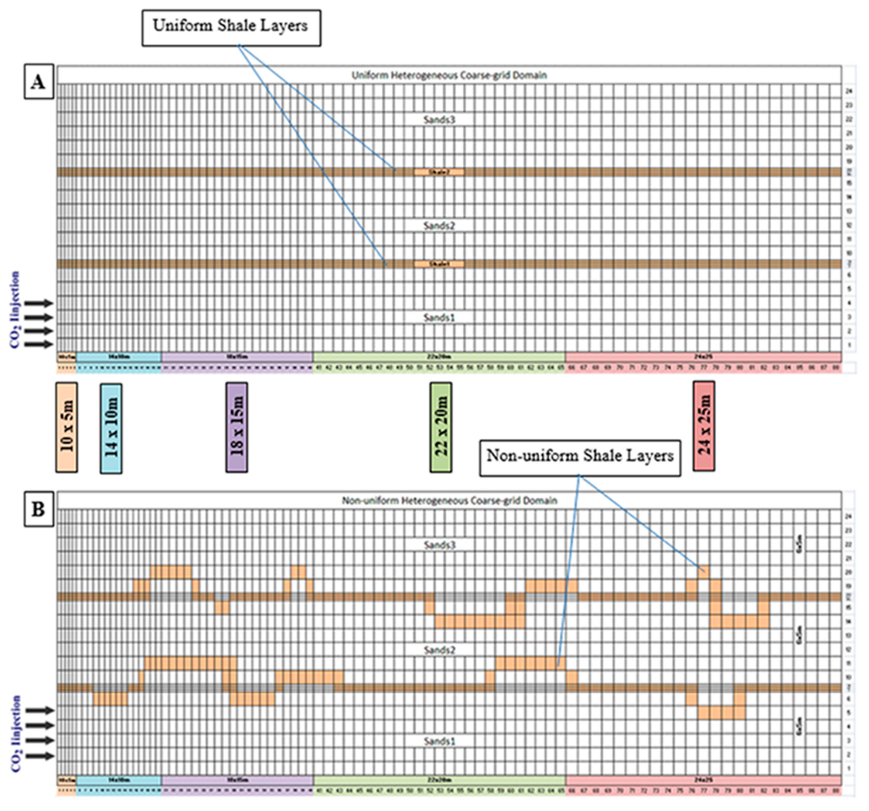
To assess the storage capacity and efficiency of an unconfined aquifer (i.e., migration-limited domain), a hypothetical cylindrical computational domain, extending from 0.3 m (the radius of the injection-well case) to 6000 m laterally and 96 m vertically, was simulated with two types of numerical grid resolutions, namely, coarse and fine grids. For the coarse-grid, the domain was horizontally discretized into 88 grid-blocks with a finer mesh in the vicinity of the injection well, which became gradually coarser further away. Vertically, the domain was discretized into 24 blocks of 4 m high. This mesh refinement has made 2112 elements as shown in
Figure 1. For the fine resolution, the grid spacing was increased by 100% in both directions, producing 8448 cells. Supercritical CO
2 (scrCO
2) was injected into the centre of the domain at a constant rate of 32.0 kg/s (about 1 MMT/year), which represents a typical benchmark value [
38], via a number of cells either at the bottom section or through the whole thickness of the reservoir.
Heterogeneity is defined as the variability of porosity/permeability within the simulated domain and is usually quantified using various geostatistical techniques, including the Lorenz coefficient (
Lc) and the coefficient of variation (
Cv) methods that are commonly used in establishing porosity and permeability models in exploration. For this study, this variability was not calculated because the simulation parameters were taken from geological settings for Sleipner Vest Field (
Table 1 and
Table 2).
2.1. Parameters and Calculations
STOMP-CO
2 simulation code [
42] was used to carry out the simulation runs in this research work and conduct the
Pc-Sw calculations. This has been discussed earlier [
9,
42] and therefore it is not discussed in detail in this paper and, additionally, the simulation code results were validated through a reasonable mapping with a lab-scale setup which was described in detail in a dedicated section of previous research by the authors [
44]. The simulation parameters used in this work are based on the geological settings for the Sleipner Vest Field, which is located in the Norwegian part of the North Sea at an approximate depth of 1100 m. It is identified to be one of the typical CO
2 disposal sites offering anticipated hydrostatic conditions to keep the injected CO
2 in supercritical conditions. Moreover, this depth is far enough away from the fresh water sources, which are usually located at around a 500 m depth. All petrophysical parameters and formulations factors are listed in
Table 1 and
Table 2. CO
2 properties adopted in the simulation were arranged in a data table developed from the equation of state (EOS) by Span and Wagner [
45], which is widely considered to be an accurate reference EOS for CO
2 for its ability to provide accurate results in the most technically relevant pressures up to 30 MPa and temperatures up to 523 K, the conditions that are common in the geological sequestration of CO
2.
The Span and Wagner equation is based on an extensive range of fitted experimental thermal properties in the single-phase region, the liquid–vapour saturation curve, the speed of sound, the specific heat capacities, the specific internal energy and the Joule–Thomson coefficient [
46]. This equation is expressed in the form of the Helmholtz energy (
) as follows:
where
,
,
and
are the critical density and critical temperature of CO
2, respectively.
is the ideal gas part of the Helmholtz energy and
is the residual part of the Helmholtz energy. The two parts of the Helmholtz energy (the basic and phase diagram elements) of this equation of state are explained in detail in the literature published by Span and Wagner [
45] and are not repeated in this study. The Span and Wagner EOS has been employed in this research to calculate the density of CO
2 at different simulation conditions under the following assumptions:
It is based on a wide range of experimental data with uncertainty values of +0.03 to +0.05% in the density values.
It is valid for a wide range of pressure and temperature values, even beyond the triple (critical) point in the phase-diagram of CO2.
The EOS can be extrapolated up to the limits of the chemical stability of CO2.
The only limitation of this EOS is that it is time-expensive to evaluate in dynamic numerical simulations because it consists of a large number of algorithms and exponentials.
The phase equilibria calculations in STOMP-CO
2 code [
42] are conducted via a couple of formulations by Spycher et al. [
47] and Spycher and Preuess [
48] that are based on Redlich–Kwong equation of state with fitted experimental data for water–CO
2 flow systems. The mole fraction of water in the gas phase (
) and mole fraction of the CO
2 in the aqueous phase (
) are calculated by the following equations:
where:
In Equations (7) and (8),
is the thermodynamic equilibrium constant for water or CO
2 at temperature
in Kelvin (
), and reference pressure
,
is the total pressure,
represents the average partial molar volume of each pure condensed phase,
is the fugacity coefficient of each component in the CO
2-rich phase and
is the gas constant [
42].
The aqueous saturation (
) is calculated by Van Genuchten [
49] formulation that correlates to the capillary pressure (
) to the effective saturation (
):
where
is the water residual saturation and
,
and
are the Van Gunechten parameters that describe the characteristics of the porous media.
During the injection period (drainage process), there is no gas entrapment because it only occurs during the imbibition process when the displaced water invades the domain back as soon as CO2 injection stops leaving some traces of it trapped behind in some small-sized pores. As a result, the injected CO2 can either exist as free or trapped gas.
The effective trapped gas is computed using a model developed by Kaluarachchi and Parker [
50]:
where
is the minimum aqueous saturation (irreducible water saturation) and
R is the Land’s parameter [
51] which relates to the maximum trapped gas saturation:
is the maximum trapped gas saturation that can be achieved during the drainage process. Maximum trapped gas and minimum aqueous (irreducible water) saturation are calculated by the following correlations by Holts [
43]:
where
and
are the porosity and intrinsic permeability of the medium, respectively. The aqueous and gas relative permeabilities are computed by Mualem [
52] correlation in combination with Van Genuchten [
49] formulations, according to the following Equations (14) and (15), respectively:
where
is the pore distribution index,
is the effective aqueous saturation, which is calculated from Equation (4) and
represents the apparent aqueous saturation which is defined as the sum of the effective aqueous and entrapped CO
2 saturations [
53].
2.2. Initial and Boundary Conditions
Three types of simulated domains—namely, homogeneous, uniform heterogeneous and non-uniform heterogeneous—were modelled in this study. They were assumed to be isotropic for most simulation runs and isothermal under a hydrostatic pressure gradient of 10.012 KPa/m with an open boundary condition, leading to scattered pressure build-up. The models were presumed to have no heterogeneity in the azimuthal direction, but different vertical-to-horizontal permeability ratios were studied, in some specific cases, to investigate the effect of anisotropy on the storage capacity and efficiency. The system was modelled as a 3D cylindrical domain and the results were compared to those when the system was considered as a two-dimensional radial flow to save computational time and requirements. The gravity and inertial effects were neglected.
Prior to injecting ScrCO
2 into the centre of the domain, it was considered to be fully saturated with brine with initial conditions, as illustrated in
Table 1 and
Table 2. ScrCO
2 was injected through four grid-cells at the bottom layer of the grid for 30 years, followed by a lockup period of 4970 years. No flux boundary condition was considered for the aqueous wetting phase (brine) at the injection well case as a west boundary, whilst the east boundary was set to be infinite with zero flux for CO
2 as a non-wetting gas phase. Zero flux was also considered at the top and bottom confining layers, forcing the injected CO
2 to swell crossways.
As an open storage system, the pressure build-up was not considered to be a limiting factor; however, the value of the maximum bottom-hole pressure at the injection well and hydrological effect on shallow groundwater sources had to be taken into consideration [
23,
54]. The injection rate for this simulation system was set according to the rock fracture pressure (
) using the simplified model adopted by Szulczewski et al. [
55], which calculates the pressure-limited storage capacity by:
where
is the density of the injected gas,
and
are the height and width of the domain, respectively,
represents the intrinsic permeability, and
is the compressibility of the formation;
is the bulk viscosity and
is the fracture pressure.
For infinite aquifer, the value of the maximum dimensionless pressure
in Equation (16) was ~0.87, according to Szulczewski et al. [
55].
All parameters in Equation (16) were known, except for the fracture pressure of the rock, which can be defined as the effective vertical stress for deep aquifers and is determined by the following equation, given by Szulczewski et al. [
56]:
where
,
represent bulk and brine densities, respectively, and
Z is the depth at which the aquifer is located.
where
is the rock density and
is the formation porosity.
From Equations (16)–(18), the value of the injection rate for the model is set at 32 kg/s, which, according to Equation (16), results in a pressure build-up value of less than 1.5 magnitudes of the hydrostatic pressure. This value is far away from the average default values of the sustainable pressure (181% of the hydrostatic pressure gradient) reported for Dundee Limestone in the Michigan Basin in the USA, which is located at a 1200 m depth [
23].
2.3. Storage Efficiency Calculation
Theoretically, the CO
2 sequestration efficiency in saline aquifers can be assessed by calculating the efficiency storage factor, which refers to the volume fraction of the pores occupied by the injected CO
2:
is the volume of injected CO
2, which can be calculated from the known mass rate of the injected gas under the hydrostatic conditions of the geological formation.
is the volume of the pores in the domain:
where
and
are the total volume and total porosity of the domain, respectively.
To calculate the storage capacity in this research work, the modern equation, developed by Szulczewiski [
34], was employed:
where
is the total mass of the integrated CO
2 (dissolved and residually trapped),
is the density of CO
2 at hydrostatic conditions and
represent the width, total length and net thickness of the aquifer, respectively.
defines the porosity of the rock and
defines the connate (irreducible) water saturation.
This methodology has been implemented because it accounts for the net thickness of the aquifer rather than the whole thickness. This can be justified by the fact that only the higher permeability layers are targeted by the injected gas [
34].
This study aims to investigate the impact of heterogeneity, permeability, grid resolution and injection methodology on CO
2-water system mobility and the behaviour of the injected scrCO
2 at different time steps on the CO
2 storage capacity and efficiency at a field-scaled domain. An archetype of actual field heterogeneity has been developed in a domain that consists of three stratums of sands intermingled with two layers of low permeability shales, as illustrated in
Figure 1. All petrophysical and simulation parameters are shown in
Table 1 and
Table 2, respectively.
A series of simulation cases (presented in
Table 3) were setup to demonstrate different models of a computational domain, including homogeneous, uniform and non-uniform heterogeneous models with coarse and fine grid resolutions. The simulation runs comprised two different employed schemes of injection (continuous and cyclic). The continuous injection scheme involved 30 years of continuous injection at a constant rate of 32 kg/s (about 1 million metric tons (MMT) per year) while in the second scenario, the injection period was implicated in three cycles of 10 years, separated by two stopping periods of 5 years in between in order to ensure that the structural trapping mechanism ended and other trapping mechanism took their role before injecting a new cycle. Furthermore, three cases with different values of vertical-to-horizontal permeability ratio (
kv/
kh) were developed along with other models to assess the influence of injection scope and orientation of the injection well on the flow behaviour and CO
2 sequestration efficiency. In all 14 cases, the total simulation time was 5000 years, including injection and pausing times. This value was set up after many trial simulations to detect the steady state time scales. Before 1000 years, most of the injected gas would be in a free gas phase, which is subject to escape through any existing cracks or faults in the caprock. As the permanent sequestration of the injected CO
2 is the focus of this work, a new term of permanent sequestration factor of the aquifer (
) was introduced. This factor was calculated from the numerical simulation results by STOMP-CO
2 code [
42] and compared for different cases under different conditions through various time scales.
Due to the density difference between the injected supercritical CO
2 (scCO
2) (about 280 kg/m
3) and the existing brine (about 1100 kg/m
3) (i.e., gravity driving forces), initially the former fluid percolates upwards to be physically trapped under the upper impervious layer (caprock). During this time, part of the gas dissolves in the existing brine to form an aqueous phase rich in CO
2, which is heavier than the ambient liquid and hence sinks down to settle at the bottom of the aquifer. As soon as the injection stops, the replaced brine invades the domain to reinstate the CO
2, leaving some traces of it behind in some small-sized pores in a process called residual or capillary trapping. These amounts of CO
2 are determined by the simulation code for different cases and utilized to calculate the capacity and efficiency of the simulated aquifer. The latter values are used to calculate the sequestration efficiency by:
where all parameters are explained in Equation (21).
Because the system was assumed to be boundless (open boundary conditions) with no pressure build-up, most of the integrated free gas was subject to migration away from the injection well along the overlapping layer and a small amount of it may sweep out of the domain through any existing fractures or faults in the overlaying caprock. Therefore, in this work the focus was on the storage efficiency of the aquifer in terms of the permanent sequestration of the injected CO
2, which occurs mainly through solubility and residual trapping mechanisms due to the insignificant influence of the mineral trapping mechanism for a few thousand years, according to De Silva et al. [
39].
3. Results and Discussion
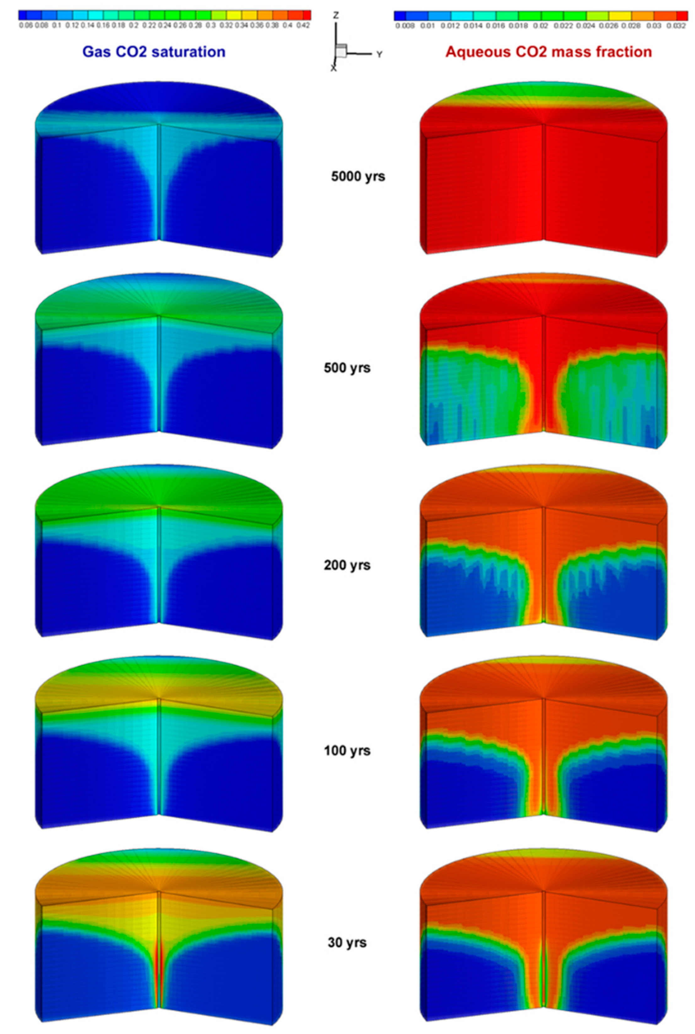
Injecting scCO
2 into a brine-saturated porous formation produces spatial distribution maps of both fluids.
Figure 2 illustrates the integrated gas saturation maps and spatial distribution of the aqueous CO
2 mass fraction within the 3D cylindrical model of the simulated domain (case Base-3D in
Table 3) at different time scales. It is shown that, soon after injection, the gas bounces upwards due to the density difference between the two fluids and simultaneously migrates crossways due to the pressure gradient between the injected ScrCO
2 and the in situ hydrostatic pressure. During this drift, some of the injected gas disperses into the existed brine, producing a CO
2-saturated aqueous phase that is heavier than the pure brine and, consequently, tends to sink down towards the bottom of the domain, forming a fingered structure, as displayed in
Figure 2 (right).
3.1. CO2 Mobility and Behaviour
Due to the density difference between the injected gas and the hosted brine, the buoyancy forces initially dominate the water–CO2 flow system. The injected scrCO2 displaces the existing brine soon after the injection starts, and the gas moves upwards to be physically trapped under the overlaying impermeable layer (caprock). The flow system involves interfacial contact between the two fluids that results in considerable amounts of the free CO2 gas to dissolve in the accommodated brine representing the solubility trapping mechanism. This is in addition to the amount of the gas that is trapped because of the capillarity and interfacial forces between the pore surface and the percolating gas.
Simultaneously, limited traces of CO2 trapped in the locale (space) even during the injection lifetime due to the injection pressure that forces some drops of the gas into some small-sized pores. However, these amounts are insignificant and further subject to be snapped off by the invading brine during imbibition. The actual capillary trapping is noticeable only after the gas injection stops. As soon as the injection ceases after 30 years, the residual trapping mechanism dominates when the replaced brine invades back the domain to sweep the integrated gas out of the pores. During this process, traces of CO2 get detached from the trailing part of the gas plume and pierce into the small-sized pores due to the capillary forces.
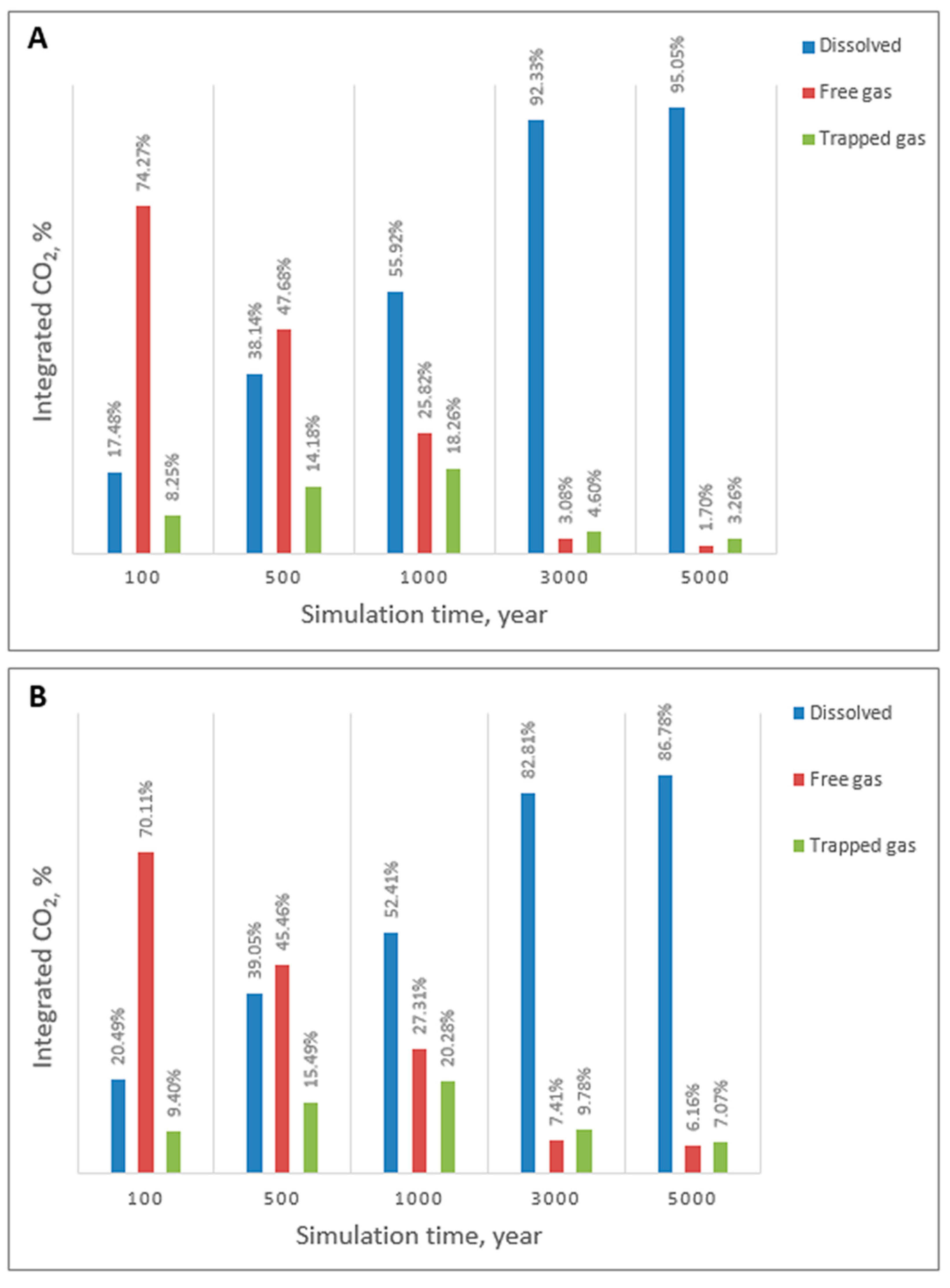
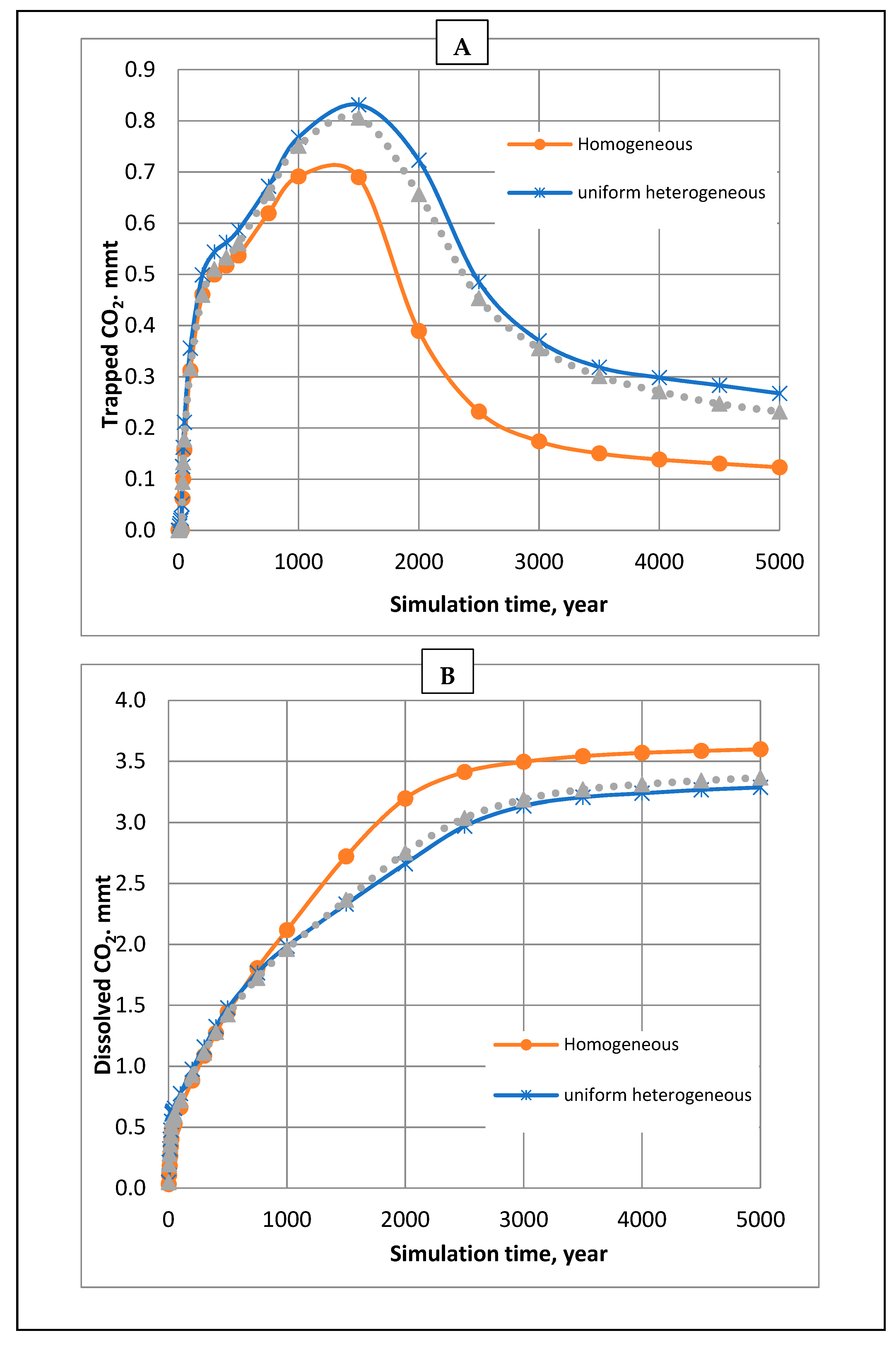
The displayed trends in
Figure 3A exhibit that, after 100 years, ~74% of the injected scrCO
2 was structurally trapped as a free integrated gas in the homogeneous domain. ~17.5% of the injected CO
2 was dissolved in brine and the remaining 8% was residually trapped in small-sized pores due to the capillarity. For the heterogeneous model in
Figure 3B, on the other hand, it was observed that ~70% of the injected gas was trapped as a free gas, 20.49% was dissolved in the brine, while 9.4% was disconnected from the plume trailing edge and adhered to the rock surface inside some small-sized pores, due to the surface tension forces.
The findings from this study have shown that, under similar hydrostatic conditions and petrophysical characteristics, homogeneous formations promote more CO
2 dissolution, owing to the fact that, under the same hydraulic gradient, fluid flows faster in homogeneous porous media compared to that in the heterogeneous porous medium, which limits fluid seepage and is consistent with some previously published studies [
57,
58].
This fast migration induces more contact with fresh brine, leading to the higher dissolution rates of CO
2. This can be seen in
Figure 3A,B, which shows that only 1.7% of the injected CO
2 was left as a free gas in the homogeneous model at the end of the simulation compared to the heterogeneous case, in which more than 6% of free gas was recorded.
The timing maps of CO
2 sequestration by each trapping mechanism are depicted in
Figure 3 for homogeneous and heterogeneous formations. It can be seen from the figure that, during the first few hundreds of years, the structural trapping mechanism dominates (i.e., more free CO
2 gas) while, after thousands of years, the solubility trapping becomes the dominant mechanism (i.e., more CO
2 dissolves in the brine). The maximum amount of CO
2 is residually trapped at about 1000 years and declines later because some of it dissolves into the surrounding brine to form weak carbonic acid that reacts with the rock material and precipitates as solid carbonates after a few thousand years.
3.2. Impact of Heterogeneity
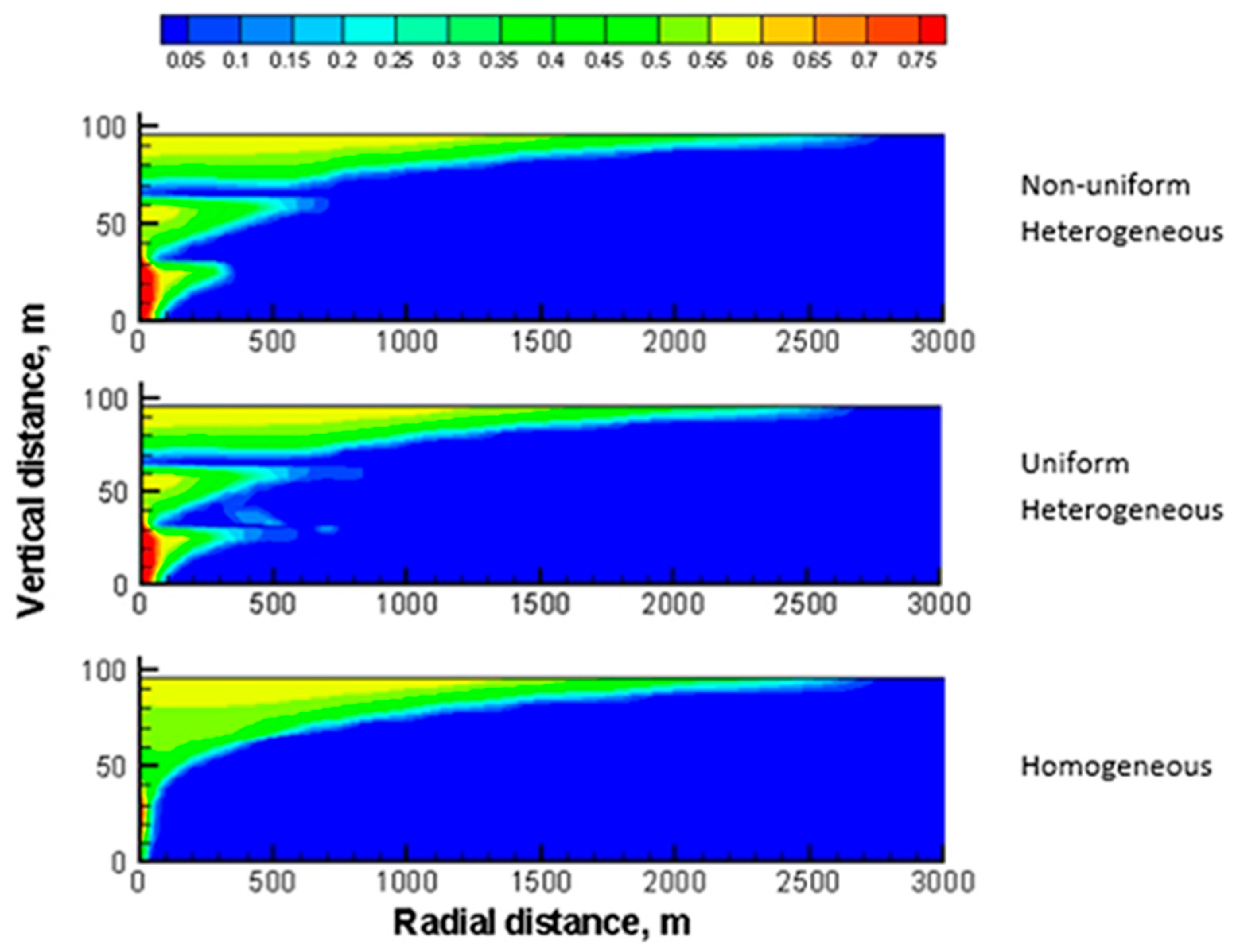
To investigate the impact of different types of heterogeneity (uniform and non-uniform) on the propagation of CO
2 profiles,
Pc-Sw relationships and storage efficiency, three numerical cases—namely 1, 2 and 3—with their employed conditions, illustrated in
Table 3, have been implemented in this study. It is a fact that the permeability of geological formations is strongly dependent on their porosity and heterogeneity, and it plays a key role in understanding water–CO
2 flow in the subsurface. This influence is clearly exposed in
Figure 4, which demonstrates different maps of gas distribution in the modelled domains.
The achieved maps depict that the homogeneous domain has produced sharp-edged contours, while the heterogeneous media resulted in irregular edges exposing more contact surface area between the CO2 and the local brine, which enhances the storage efficiency. The irregular frontages in the heterogeneous media are due to the intermingled layers of shale that restrict the injected gas from moving across different layers of the domain that results in less contact with the ambient brine and less subjectivity to entrapment in more small-sized pores. Heterogeneity is found to have a substantial impact on the amounts of trapped and dissolved gases, as a result of the influence on the capillary pressure–saturation relationship, which is imitated by an increase in the amount of the residually trapped CO2.
Figure 5A shows that, soon after gas injection stops (i.e., imbibition process starts), the amount of the trapped gas sharply increases when the replaced brine invades back into the domain and isolates some blobs of CO
2 from the trailing edge of the mobile CO
2 plume. After 200 years, this progress slightly retards because part of the trapped gas tends to dissolve in the brine. This increase continues until 1400 years of simulation, when the trapped gas profiles steeply decline before tending to settle after 3000 years. The figure further demonstrates more residually trapped gas in the heterogeneous models compared to the homogeneous ones at the end of the simulation.
In
Figure 5B, no effect of heterogeneity on CO
2 solubility was detected before 800 years of simulation because the system was totally dominated by buoyancy and hydrostatic forces. Afterwards, it was observed that more CO
2 got dissolved in the homogeneous domain compared to both types of heterogeneous ones by about 17% after 2000 years. However, this influence approximately declined after 4000 years to 9%. It is apparent from the results, displayed in
Figure 5B, that both types of heterogeneity provide almost identical but lower amounts of dissolved CO
2 compared to the homogeneous media throughout the simulation time. This suggests that gas migration is more straightforward through homogeneous media, owing to the lesser resistance to flow.
In contrast to the results by Chasset et al. [
35], the increase in CO
2 dissolution can be justified by the presence of intermingled layers of shale that play a role as internal barriers to retard the vertical migration and the promote lateral flow of the injected CO
2. However, this horizontal movement retards after the injection period due to the limited hydraulic gradient, which limits gas contact with more fresh brine, leading to a reduction in gas assimilation and dissolution. The values of trapped and dissolved CO
2 surely affect the storage capacity of the site; however, this impact is applicable to a very limited extent in agreement with the results from a recent study by Zhao et al. [
58], which revealed that strong heterogeneity in geological formations reduces the storage capacity because it limits gas seepage.
In spite of the two contrary trends,
Figure 6, shows that heterogeneous domains are more efficient in storing the disposed gas by a factor of about 15% compared to the homogeneous ones under similar conditions. This does not comply with the numerical results depicted in
Figure 3, that show higher values of free-gas CO
2 left off by the end of simulation in the homogenous domain compared to the heterogeneous one. This controversy is due to the net thickness parameter suggested by Szulczewski [
34] for Equation (21) instead of the total thickness of the modelled domain. To implement this in our calculations, the thicknesses of the shale layers were excluded and this resulted in less values of the net thickness in cases 2 and 3 (see
Table 3), leading to smaller pore volume available to store the injected CO
2 and, consequently, higher values of storage efficiency were achieved for the heterogeneous domains using Equation (21). This is an important point that needs further investigation to assess the effectiveness of this method to more accurately determine the storage efficiency in open-boundary domains.
3.3. Effects of Cyclic Injection on CO2 Mobility and Sequestration
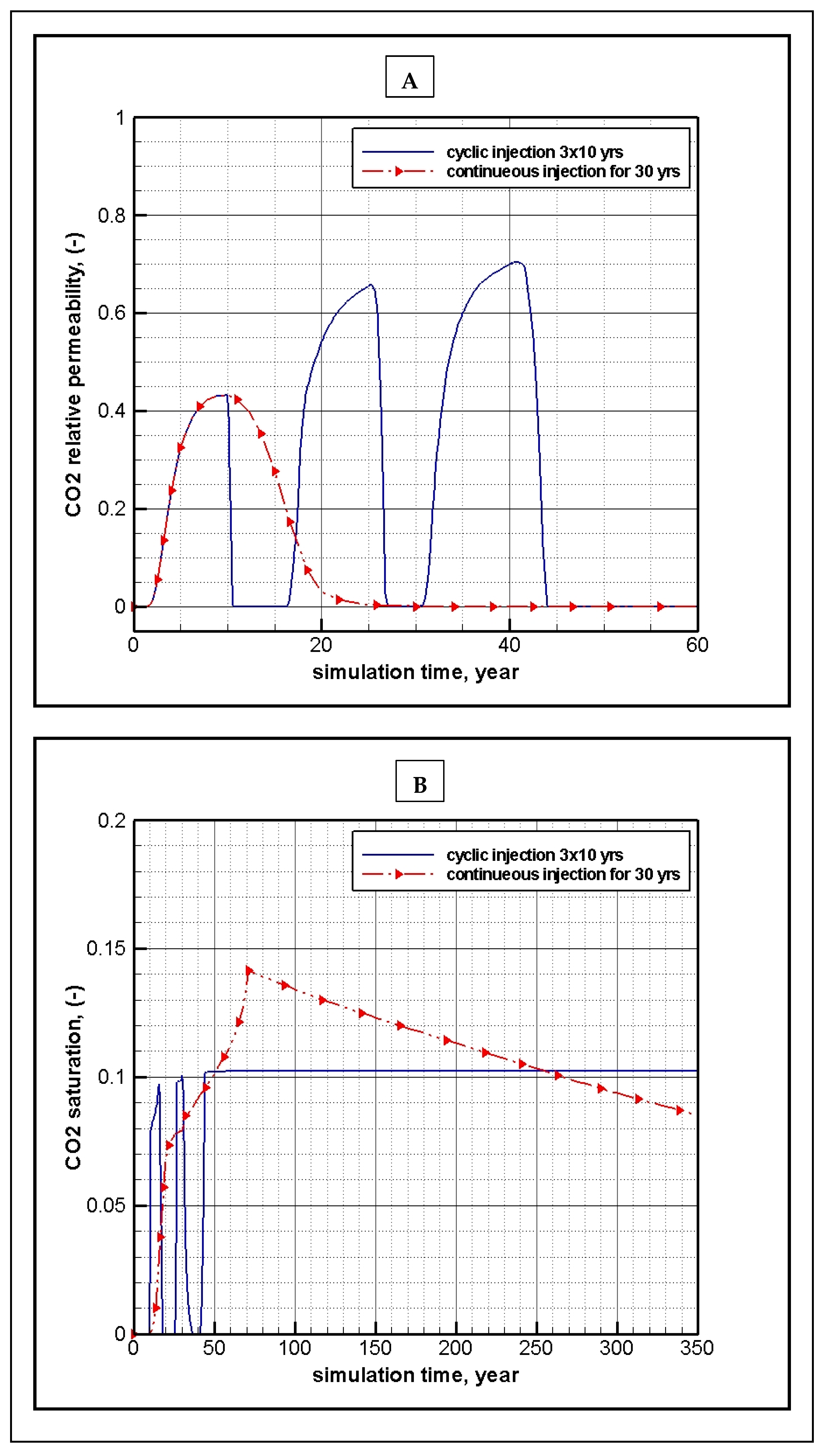
Saturation (Sw)—relative permeability (kr) relationship is a key feature that describes the CO2–water flow system because it has a huge influence on the behaviour and fate of the injected gas in the subsurface. This study has investigated the impact of the injection methodology on the Sw-kr relationships and eventually on the effectiveness of the disposed gas storage. Purposely, an observation point was setup at 200 m radially away from the injection well (to avoid the effect of the high pressure difference forces close to the wellbore) and 15 m from the bottom of the aquifer, which represents the midpoint of the lower segment of the domain into which the gas injection takes place.
The achieved results from implementing cyclic injection techniques are demonstrated in
Figure 7A, that manifests the development of gas relative permeability profiles for continuous and cyclic injection methods (see cases 3 and 4 in
Table 3). The influence of the cyclic injection is obvious from the fluctuating profiles from which it can be observed that, for the continuous injection method, the relative permeability of the CO
2 curve declined from a peak value of (0.43) after 10 years to zero by the end of the injection period (30 years). The figure further displays the three cycles of injection impact on the permeability curves with highest peak values of 0.43, 0.66 and 0.7. This impact has been directly imitated on the gas saturation trends in
Figure 7B, which evidences the favourite of cyclic injection method because higher amounts of injected CO
2 were found to be safely trapped after the cease of injection.
This is comparable to the continuous injection case, which depicts higher values of gas saturation after the end of injection; however, these values decline soon after that to reach a value of 0.01 after 2000 years of simulation (this is not shown in
Figure 7B, which is magnified to show more details about the drainage period).
This variation can be justified by the two additional cycles of imbibition process that lead to more blobs of CO2 getting disconnected from the trailing edge of the ascending gas plume.
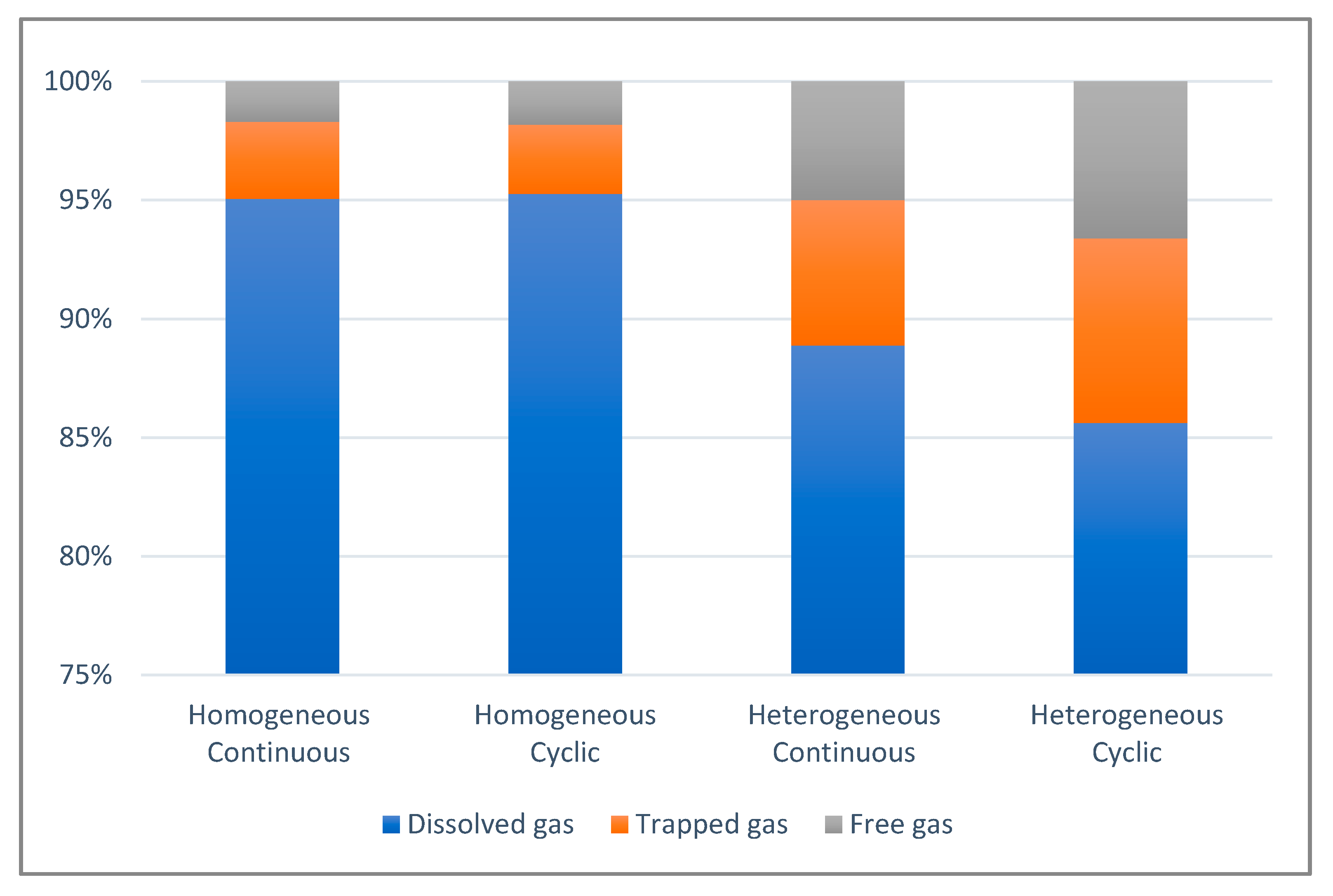
For the homogeneous models (see cases 1 and 5 in
Table 3), cyclic injection confirmed no effect on CO
2 dissolution and almost equal amounts of free gas were left off in the domain by the end of the simulation runs, as shown in
Figure 8. However, for the heterogeneous domains (cases 3 and 4), continuous injection produced slightly greater profiles of CO
2 dissolution.
In contrast, the residual trapping of CO
2 in heterogeneous media was found to be more sensitive to the cyclic injection because the simulation results revealed that more CO
2 was trapped using the cyclic injection method in the heterogeneous modelled domain compared to the continuous one after 5000 years of simulation, as illustrated in
Figure 8.
Table 4 concludes that cyclic injection into homogeneous domains increases the amount of trapped CO
2 gas to some extent (compare cases 1 and 5). However, continuous injection into heterogeneous formations enhances the storage efficiency factor (determined by Equation (21)) by about 0.0003, that represents 1.7% (compare cases 3 and 4), because it can be seen from the table that by applying continuous injection (case 3), 0.773 MMT (approximately 0.17%) more of the injected gas was permanently sequestered either by residual or solubility sequestration mechanism using continuous injection techniques.
In agreement with the results by Juanes et al. [
59], this can be justified by the increase in capillary pressure which forces more CO
2 into smaller-sized pores to be trapped and exposed to dissolution in the brine at later stages of storage. In contrary for the cyclic injection, releasing pressure after 10 years encourages the gas plume to percolate upwards through larger pores to accumulate at the top of the domain as a free gas.
3.4. Effect of Vertical Injection
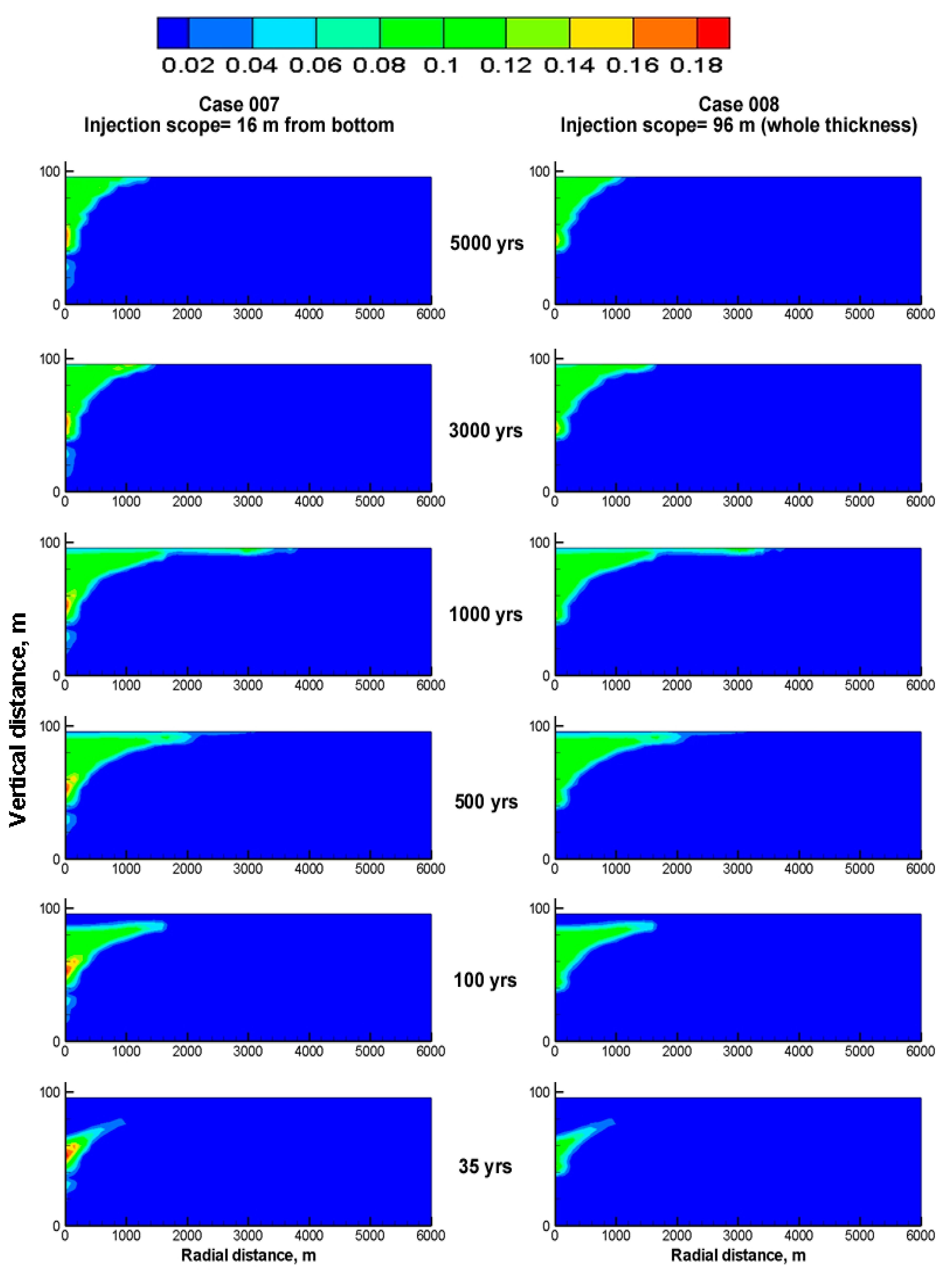
This section extends a previous work [
9] to further optimize the vertical injection method with the aim to investigate the storage efficiency enhancement. To carry this out, two simulation cases were conducted, implementing two different scopes of vertical injection (see cases 7 and 8 in
Table 3). In case 7, scrCO
2 was injected into the lower segment of the aquifer through four vertical grid cells of 4 m, while for case 8, the injection was executed over 24 blocks (i.e., over the whole thickness of the aquifer that extends to 96 m).
In terms of the dissolution of the injected scrCO
2, unexpectedly no significant effect was observed at all-time scales for case 7. On the other hand, slightly more trapped gas concentrations within the vicinity of the injection well were demonstrated for case 8, as shown in
Figure 9. This is because, in this case, the whole amount of the gas was injected through the lower segment of the domain, most of which was influenced by the reversing brine tendency to disconnect more blobs of CO
2 from the rambling edge of the gas plume. In contrast, when the injection applied into the whole thickness of the domain (case 8), only a sixth of the scrCO
2 mass rate was injected into the lower section of the model and most of this amount had bounced upwards before the imbibition process started. This means that only a significantly small part of the injected gas was affected by the raiding brine, leading to a reduced amount of residually trapped gas. It is evidenced from the achieved results that injecting CO
2 through the whole thickness of the domain slightly reduced the amount of the free gas left within the domain in medium terms of storage by 0.028 MMT (about 3.2%) as depicted in
Table 4 for cases 7 and 8. However, the injection scope has shown no sensible influence on the storage efficiency because both cases returned almost identical values of storage efficiency factor, as presented in
Table 4.
3.5. Impact of Directional Permeability Ratio
In the aim of assessing the effect of heterogeneity anisotropy in geological formations on the efficiency of storage, three models of a hypothetical aquifer with values of vertical-to-horizontal permeability ratios (
kv/
kh) equivalent to 1.0, 0.1 and 0.01 were developed and modelled (see cases 8, 9 and 10 in
Table 3). This array was set up as a realistic figure for most sandstone rocks according to a relatively new study by Widarsono et al. [
60].
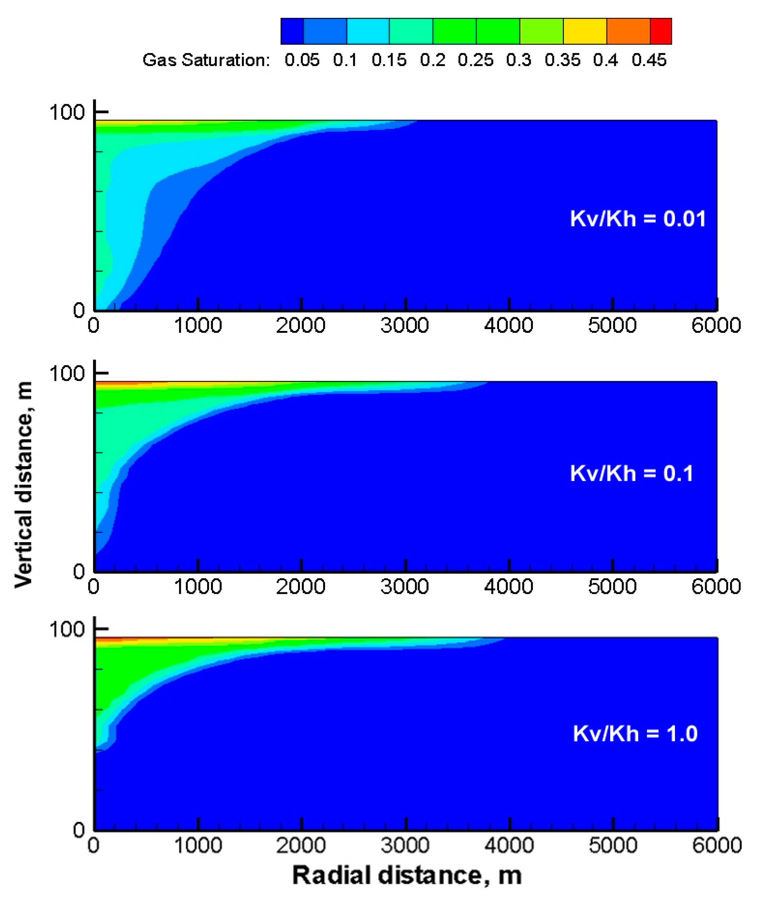
The obtained results depicted in
Figure 10, show the deceptive influence of the permeability ratio on the CO
2 plume shape and spatial distribution maps. While the plume tends to horizontally extend further along the overlaying layer at higher permeability ratios, more CO
2 shows the tendency to migrate laterally within the two lower layers of the domain for lower values of permeability ratio. This owes to the fact that lower permeability in the vertical direction restrains the upward movement of CO
2, forcing the injected gas to migrate horizontally across the domain, proposing more gas into small-sized pores where it is more likely to be permanently entrapped when the brine invades back into the domain after the injection stops, which is referred to as residual trapping.
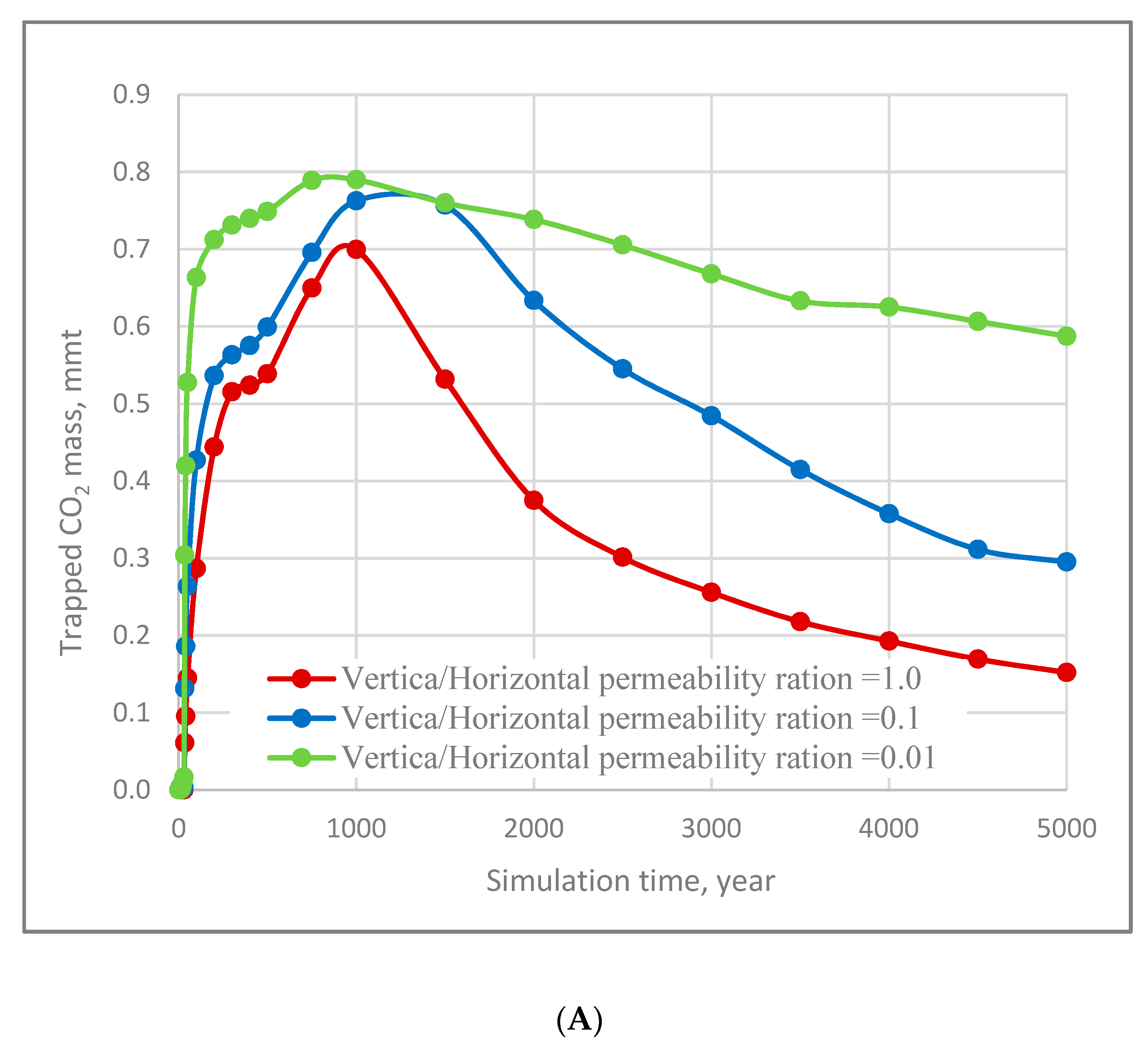
The latter impact is evidenced in
Figure 11A, which shows significantly greater amounts of trapped gas in cases of lower permeability ratios at all post injection time steps.
One of the stupendous returns from this study is the inflection point in the gas dissolution trends after around 800 years of the simulation lifetime, as noticeable in
Figure 11B. This deviation occurred because at early stages, the flow system was entirely dominated by the structural trapping mechanism, in which most of the injected gas remained in free phase. This mechanism is mainly dependent on the upwards movement of the free gas that is more effective at higher vertical permeability values (i.e., larger values of (
kv/
kh)), as explained previously in this section. The horizontal movement of the gas, due to the pressure gradient and low vertical permeability, promotes more contact between the two fluids, leading to more dissolution of CO
2 in the formation brine at early stages (solubility trapping). However, this migration has no significant impact compared to the large buoyancy forces at later stages.
This clarifies the larger amounts of dissolved CO
2 at lower values of
kv/
kh before 800 years in
Figure 11B. By approaching 1000 years of simulation, the solubility trapping mechanism takes control because the density and pressure gradient driving forces decline when most of the integrated gas has either settled at the top of the domain or within the vicinity of the injection well, as illustrated in
Figure 10 (see case 8 in
Table 3). Consequently, the domain becomes dominated by the solubility trapping, which is based on the contact interfacial area between the two fluids and the hydrostatic conditions that influence the CO
2 dissolution rate in the surrounding brine. CO
2 dissolution into the formation brine creates a denser aqueous phase that tends to sink downwards when the vertical movement becomes important to maintain more gas contact with the fresh brine, leading to more dissolution of the gas into the brine. This convectional movement is easier at higher permeability ratios that result in larger amounts of gas dissolution.
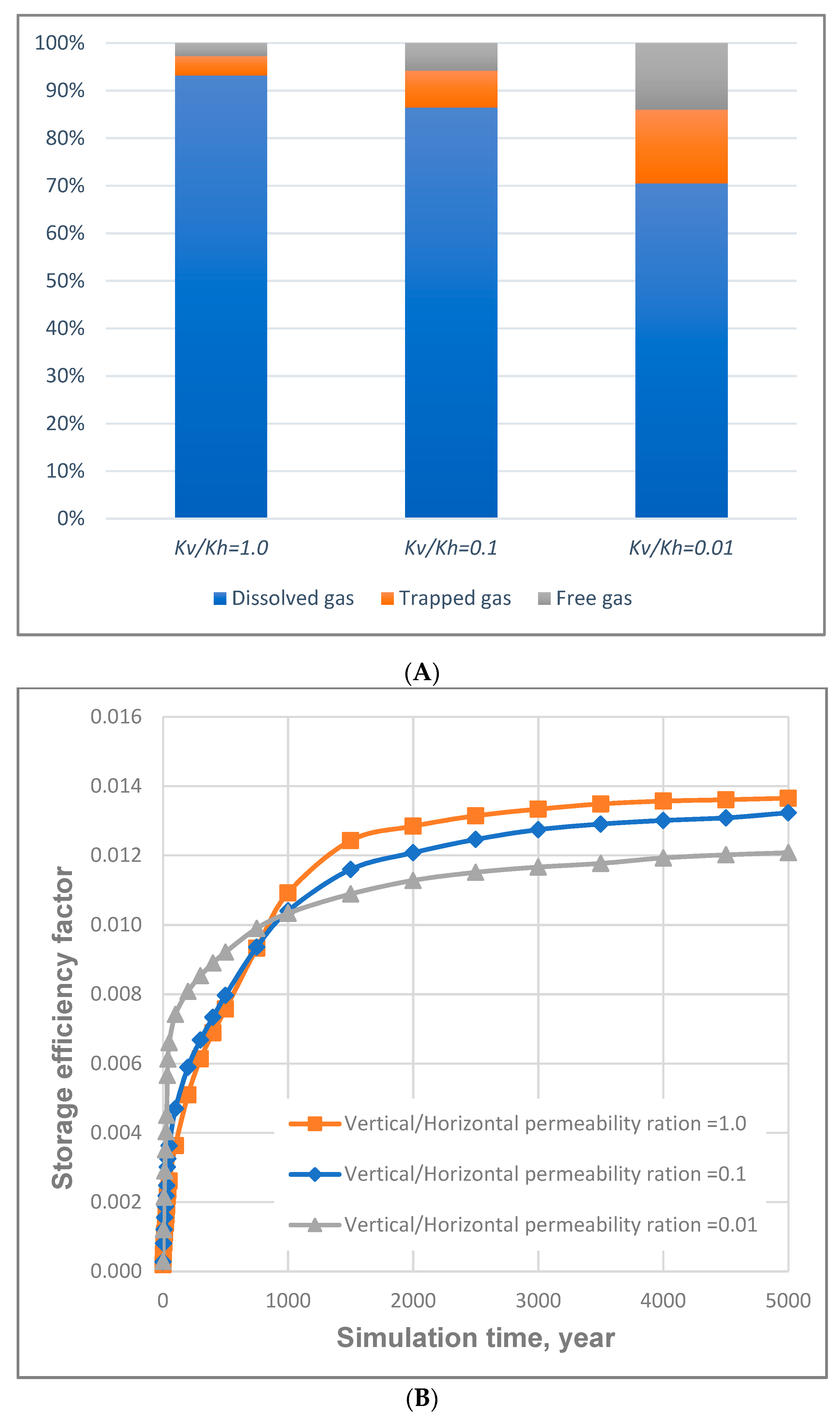
Despite all this evidence, the determined storage efficiency for different permeability ratios using Equation (21) by Szulczewski [
34] for open boundary domains has shown better storage efficiency at lower permeability ratios. This is significantly controversial and requires more investigation and discussion because our repeated numerical experiments have revealed contrasting results (see
Figure 12A,B). This can be referred to as the length parameter used in Equation (21) to calculate the effective volume of the domain and, consequently, the CO
2 mass that can be stored. The author suggested using the maximum extent of the gas plume to calculate the effective volume; however, our simulation results revealed a huge difference in the obtained plume lengths for cases 8, 9 and 10 in
Table 3. They were found to be 3965, 3802 and 3135 m for permeability ratios of 1.0, 0.1 and 0.01, respectively (see
Figure 10).
This significant difference has returned unrealistic values of the storage efficiency when implemented in Equation (21), because looking at
Figure 12A, it can be evidently noticed that higher permeability ratios produced greater amounts of dissolved and trapped CO
2, and less amounts of free-gas (i.e., enhanced solubility and residual trapping of the injected gas). It is apparent from the figure that, for
kv/kh values of 1.0, 0.1 and 0.01, the achieved permanent trapping rates were 29.457 MMT (97%), 28.55 MMT (87%) and 26.066 MMT (71%), respectively.
Depending on the findings from this study, it is suggested that the plume length parameter in Equation (21) is reviewed and presented by a more realistic value to make the equation further applicable to various CO2 injection scenarios into geological formations.
In this work, the total length of the domain, which extends far enough that the gas plume does not reach it, was used in order to avoid any boundary effects on the in situ pressure build-up or gas seepage from the computational domain for all simulation runs (i.e., to employ an open boundary condition away from the injection well). This means that the whole aquifer volume was used to calculate the storage efficiency factor, which explains the small-obtained values of the efficiency factors in
Table 4. Using this total length in Equation (21) to determine the sequestration efficiency has returned more realistic values of the storage efficiency in terms of the directional permeability effect, as shown in
Figure 12B, which indicates that the storage efficiency factor of any aquifer increases proportionally with the vertical-to-horizontal permeability ratio (see cases 8, 9 and 10 in
Table 4).
3.6. Influence of Injection Orientation
Injecting CO
2 into sedimentary formations through horizontal wells has been a subject of many research works and review studies, most of which are based on applying horizontal injection into confined geological formations, considering the induced pressure build-up. While some authors conclude that injecting CO
2 via horizontal injection wells improves the trapping efficiency [
39], others find that such a methodology influences the mechanical stability of the overlaid caprock and does not improve the storage efficiency in the long term [
40,
61].
In this study, we investigated the influence of the injection orientation on the hydrodynamic behaviour of CO
2 and storage efficiency for an open boundary model and compared the results with those for the conventional vertical injection methodology. Purposely three simulation models were developed (see cases 10, 11 and 12 in
Table 3) to identify the impact of the injection orientation on the storage efficiency and
Pc-Sw relationship in geological formations. Both vertical and horizontal injection wells were set up for 96 m for cases 10 and 11, while the horizontal well length was extended to 192 m for case 12. All other simulation conditions were similar for the three cases and a constant injection rate was maintained to run the simulations over different well lengths (96 and 192 m).
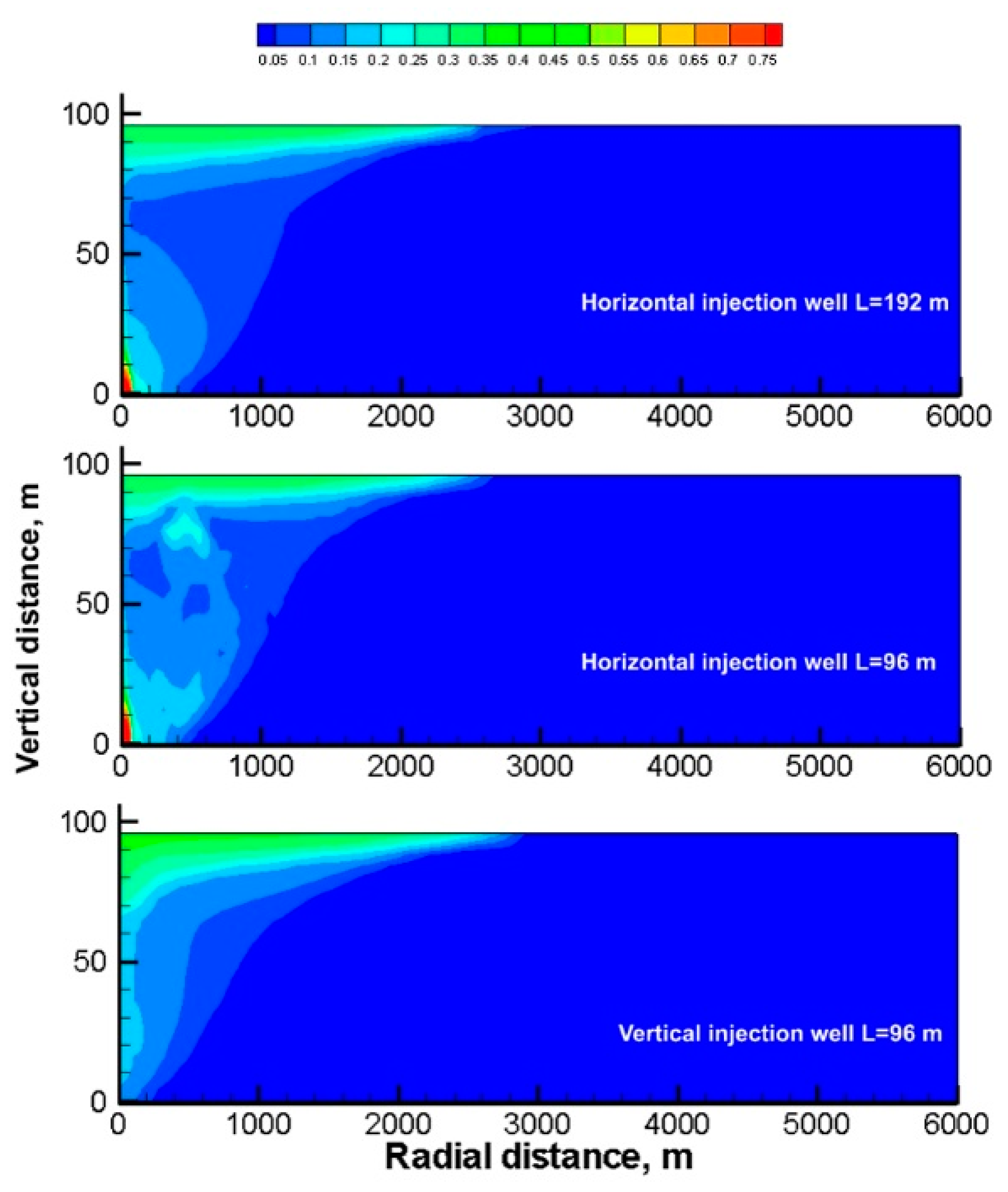
The achieved numerical results revealed that injection orientation has a significant influence on the gas migration and behaviour in unconfined geological formations, as depicted in
Figure 13, that highlights the disparity between the gas distribution contours achieved through using horizontal injection wells (cases 11 and 12 in
Table 3) and those obtained from the vertical injection methodology (case 10).
The figure exhibits that a noticeable portion of the injected gas was trapped by the displacing brine in the case of the aquifer-thickness equivalent horizontal injection well (96 m) compared to the longer horizontal well (192 m). This can be attributed to the large injection mass flow rate per unit area (i.e., limited number of gridlocks) which delayed the upwards propagation of the buoyant CO2, leading to only part of it reaching the top of the domain to create a thin tongue-like shape that migrated crossways. The other portion of the injected gas was exposed to be encountered by the invading brine that physically isolated blobs of it within the local pores network to be dissolved at later stages.
Using horizontal injection techniques was found to increase the quantities of the trapped gas, as presented in
Table 4, due to the magnified values of average capillary pressure. Unexpectedly, the amount of the trapped gas was found to be significantly less than that which was achieved by the shorter horizontal well. This can be explained by the smaller injection rate per unit area in the first case, which promotes more percolation of the free-gas towards the top of the aquifer, as shown in
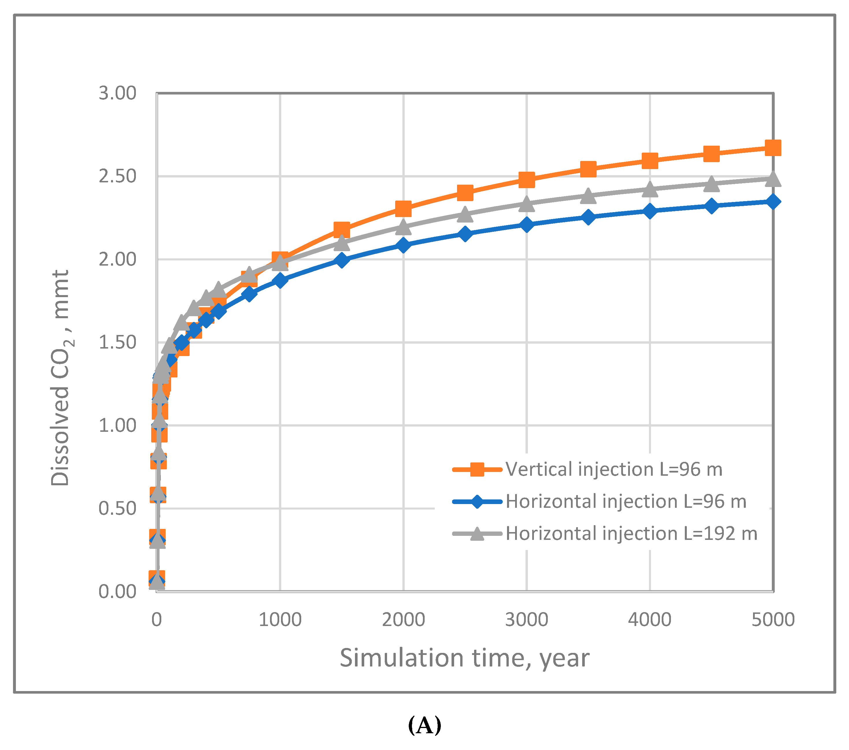
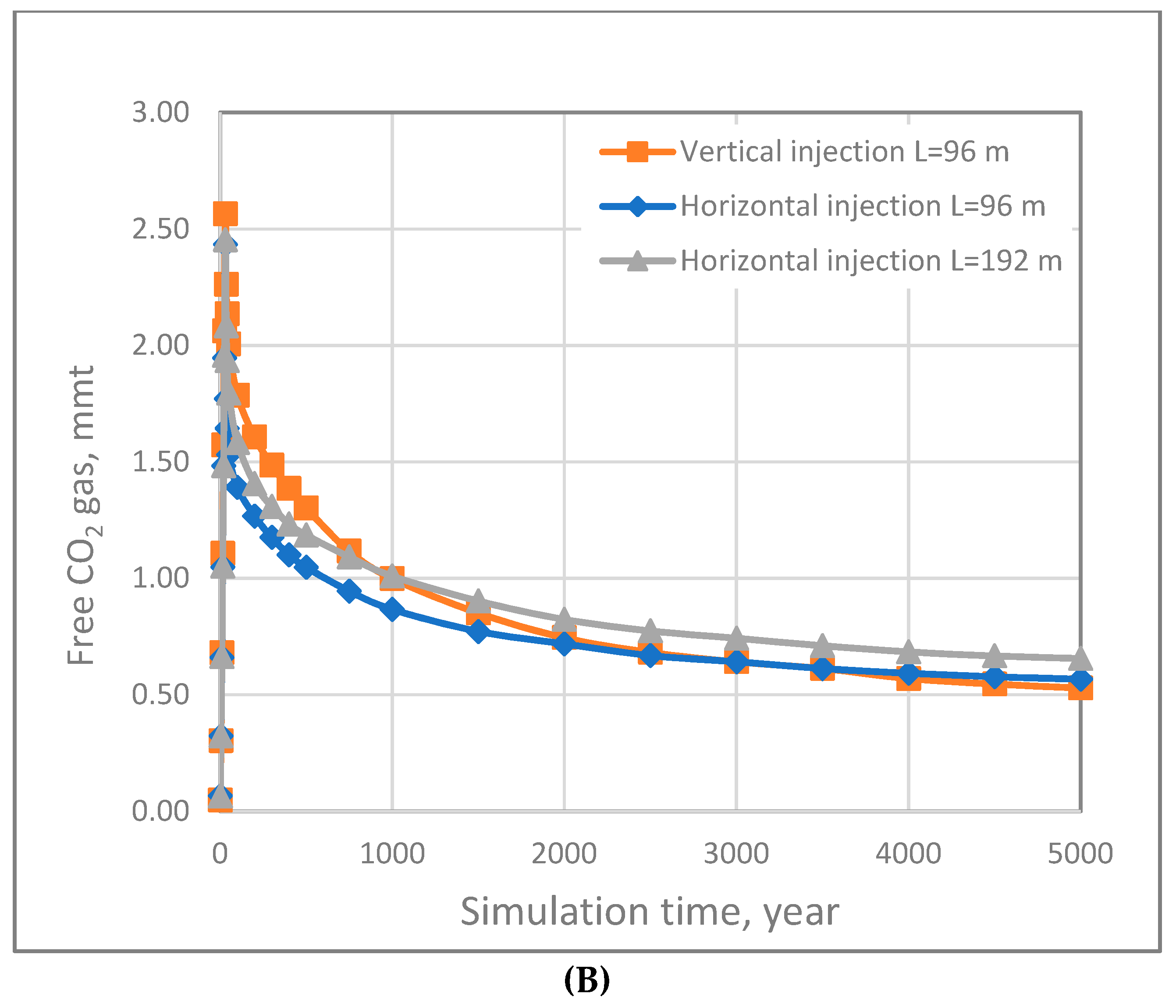
Table 4. Despite the relative increase in the gas dissolution depicted in
Figure 14A, for the longer horizontal well, the amount of the free-gas left off by the end of the simulation was higher, as shown in
Figure 14B, leading to lower storage efficiency, as evidenced in
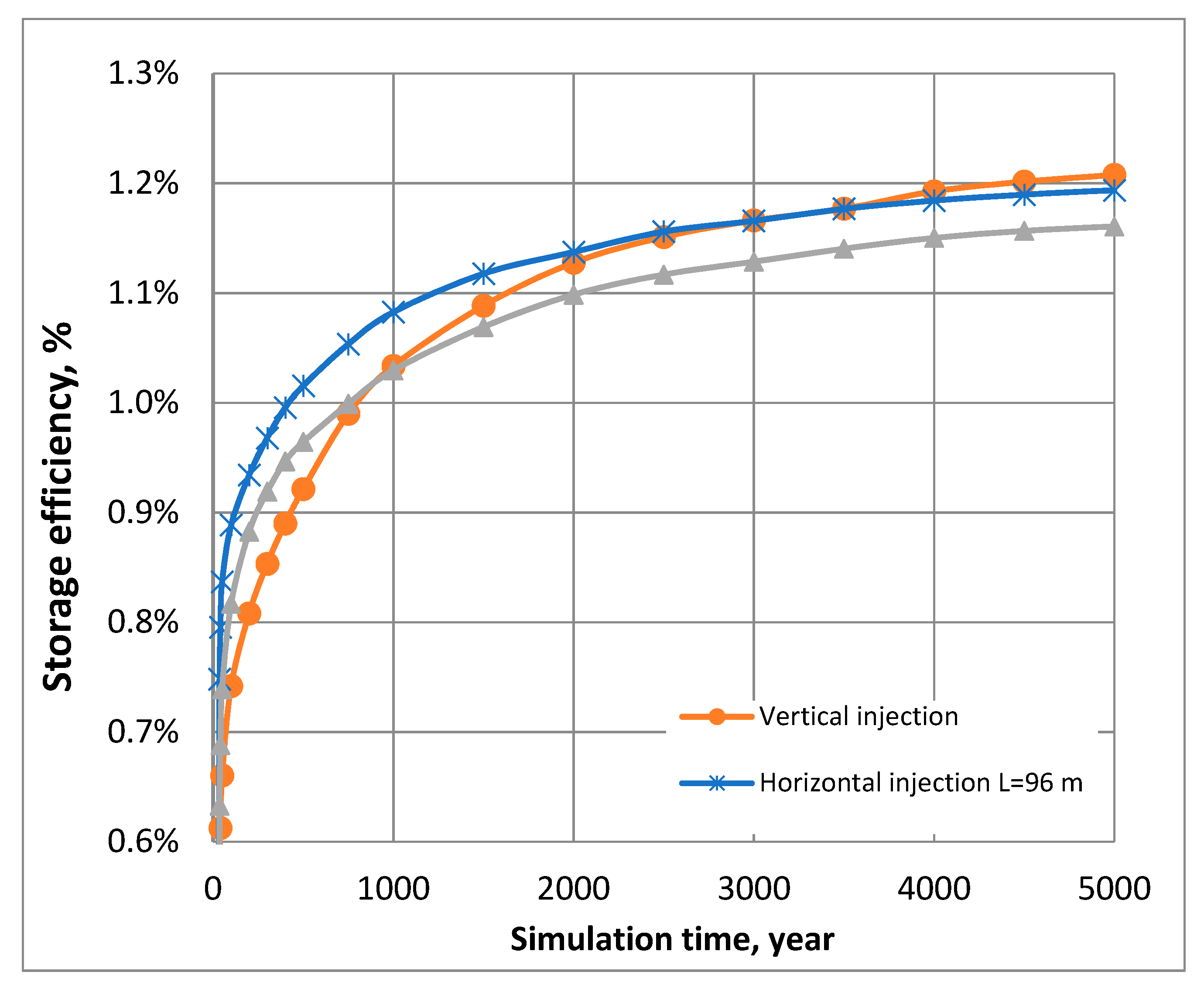
Figure 15.
Additionally, the results reveal that horizontal injection into migration-controlled domains (i.e., open-boundary domains), returns slightly higher storage efficiency in short terms of simulation; however, after 2000 years, vertical injection methodology was found to be more efficient, as evidenced in
Figure 15.
This is consistent with the findings by Okwen et al. [
61], who suggest that using horizontal wells is preferable for pressure-limited domains and for sequestering large amounts of CO
2 in a short time frame. Accordingly, implementing longer horizontal injection wells does not significantly enhance the storage capacity and the economical factor has to be taken into consideration, should they need to be used for injecting large amounts of gas within limited periods of time.
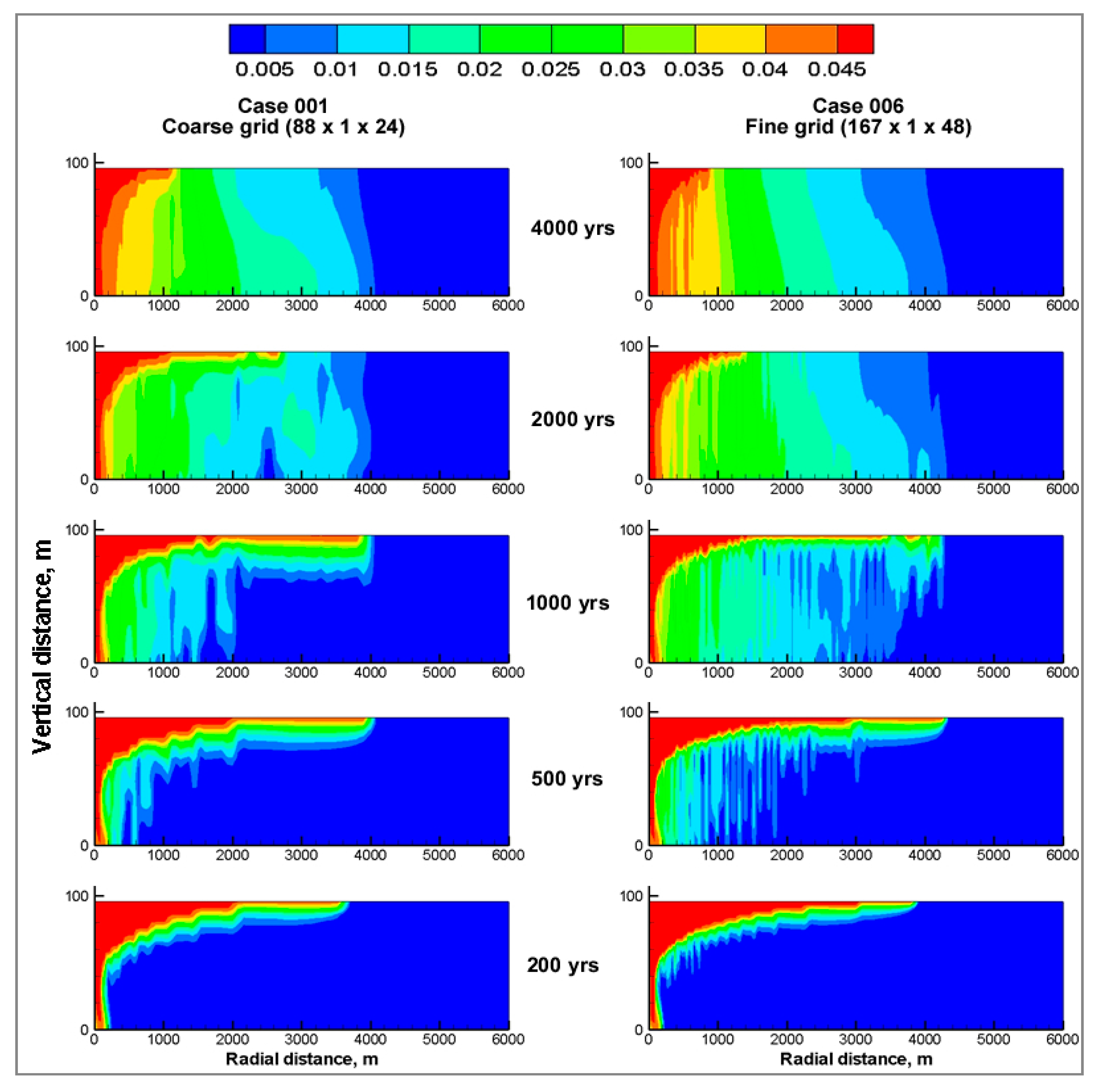
3.7. Sensitivity to Domain Grid-Resolution
The grid discretization of any simulated domain is an important factor used to accurately capture the occurrence of different flow dynamics and assess the sensitivity of modelling results to the spatial gridding schemes. As mentioned earlier, in this study, two levels of grid refinement, a coarse grid (88 × 1 × 24) and a fine grid (176 × 1 × 48) were used to record the simulation code outputs (see cases 1 and 6 in
Table 3).
The influence of the grid resolution is illustrated in
Figure 16, where more detailed fingering maps of CO
2 dissolution can be observed in the fine-grid domain, compared to those for the coarse grid. Moreover, longer gas plumes were detected in the finer grid, which means that more accurate records of different forms of integrated gas were netted.
This is further evidenced in
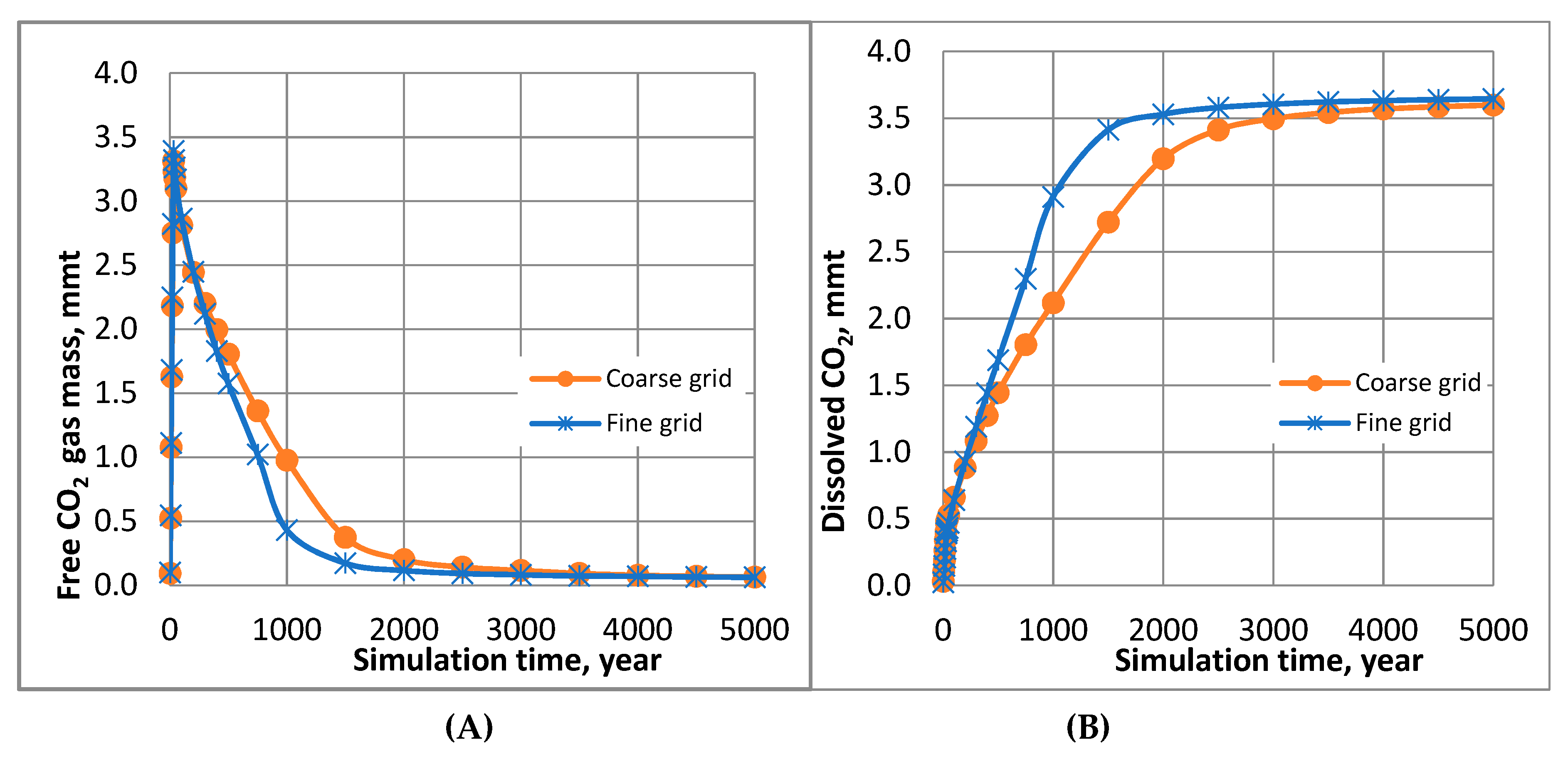
Figure 17A,B, in which it can be observed that, after 1500 years, a about 20% larger amount of dissolved gas and 54% lesser amount of free-gas were logged by the simulation code when a finer grid was implemented. These figures declined to about 1.3% and 3.2%, respectively, by the end of simulation. In
Figure 17A, less impact of the grid resolution on CO
2 dissolution in the hosted brine was noted for both grids up to around 300 years of simulation. Then, after, an obvious increase in the dissolved gas trends for the finer grid, specifically between 800–2000 years, was noted. This deviancy diminishes after 2000 years, which agrees with the findings by Gonzalez-Nicolas et al. [
62] and Bielinski [
63].
This can be justified by the findings from this work (see
Figure 15), which demonstrate the influence of grid resolution on the plume shape and number of formed fingers in the simulated domain due to the convection forces and gravity instability. Consequently, more accurate results were logged using finer grids which justifies the relatively higher efficiency achieved in the case of fine-resolution grid, as illustrated in
Figure 17.
Unexpectedly, the results revealed higher gas entrapment in the coarse grid (case 1) than that for the fine grid (case 6), as shown in
Table 4. This can be due to the fact that, by using larger blocks in the computational domain, part of the dissolved CO
2 might have been logged either as a free or trapped gas, which can be explained from the relatively larger amounts of the latter two forms of the content gas in the case of coarse refinement. In spite of this significant overestimation of the netted values of the trapped gas in the coarse grid, the amount of the free gas was found to be less in the finer grid by about 3.2%, as displayed in
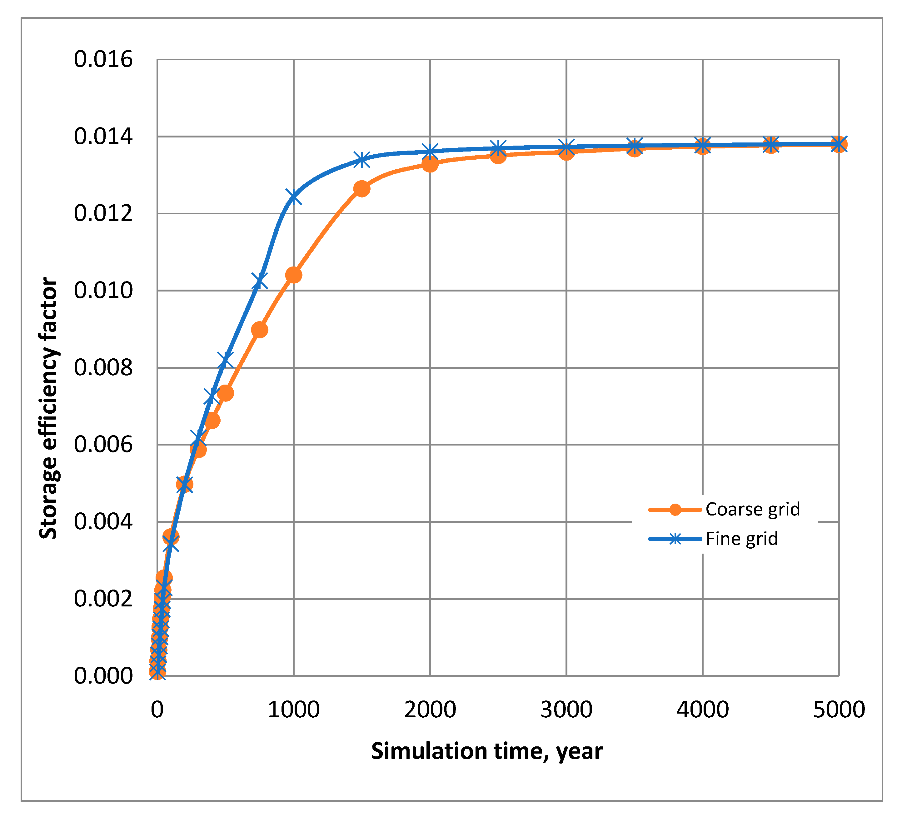
Table 4. However, the increase in the storage efficiency factor was only about 0.1% using a finer grid, as shown in
Figure 18, which further clarifies that the grid refinement has only a small impact on the simulation results. Additionally, the amount of the residually trapped gas was much smaller than the amount of the dissolved CO
2 shown in
Table 4 and, moreover, this small amount of the trapped gas itself is subject to dissolution in medium over long time frames.
Some preceding publications concluded only a slight or no impact of grid resolution on the simulation results. Conversely, ranking our simulation cases, according to the attribute of safer storage of the disposed gas in
Table 4, the finer grid case was found to be on the top of the list. Therefore, and despite the excessive execution time required to conduct simulation runs with finer grids, it is important to magnify focus on the behaviour of the injected gas in different phases (i.e., dissolved, residually trapped and free-gas) within in situ pores network by using reasonably refined grids. The results from the finer mesh (see case 6 in
Table 4) detected only about 0.497 MMT of free gas at the end of the simulation lifetime compared to about 0.514 MMT for the coarse grid in case 1, which reflects about 3.2% safer storage by the means of deploying the finer grid. This should be motivating for the researchers to refine their modelling grids for further focused and more credible accurate results. Nevertheless, it is recommended that a sensible balance between the grid refinement and the computational time required for calculations be embraced.
For the cylindrical domain modelled in this research work (3 km radius and 96 m thickness), it was found that discretizing it to 176 by 48 nodes in the lateral and vertical direction, respectively, was found to provide a reasonably effective level of refinement in terms of balancing between the accuracy of the achieved results and the computational time and requirements.
4. Conclusions
A set of numerical simulation cases was developed and conducted using the STOMP-CO2 numerical simulation code to investigate the influence of various types of heterogeneity, injection schemes, grid resolution, anisotropy, and injection orientation on the CO2–water flow system behaviour and storage efficiency in saline aquifers. It was found that heterogeneous formations amplify the residual trapping mechanism, while CO2 dissolution (i.e., solubility trapping mechanism) shows higher trends in homogeneous formations. However, overall, the heterogeneous media were found to be more effective in storing CO2 safely over long-time frames. Compared to the homogeneous media, cyclic injection methodology has shown more influence on the heterogeneous domains through which the injected gas spreads out further, leading to greater interfacial area with brine and, consequently, escalating CO2 dissolution. However, further research work is required to investigate more details about optimizing the injection times and pausing intervals in long-term sequestration projects where mineralization trapping plays an important role.
We observed that, while a CO2 gas plume extends further at higher kv/kh values, lower ratios enhance the solubility trapping of CO2 at early stages of simulation. Additionally, stronger hysteresis at higher permeability ratios enhances the residual trapping mechanism. Overall, storage efficiency increases proportionally with the permeability ratio of geological formations because higher ratios facilitate the further extent of the gas plume and increase the solubility trapping of the integrated gas. Using the maximum length of the gas plume in Equation (21) to calculate the available porous volume in open-boundary domains requires more investigation because it produced some unrealistic results. Therefore, an optimization is suggested to set up the domain length according to the employed injection rate or pressure, so that the extended gas plume just reaches but does not pass it. This length can be called the effective length and can be used to calculate the volume available to host the potential injected gas. It is also concluded in this study that employing longer horizontal wells does not increase storage efficiency. However, more research work is recommended to optimize the length of the horizontal wells and the injection techniques, including injecting chase brine along with scCO2.
Despite the excessive execution time required to run simulations on finer-grid domains, it is important to magnify focus on the behaviour of the injected gas in order to increase the accuracy of the logged results. Finer-resolution grids can slightly increase the calculated values of the storage efficiency factor, specifically in the medium terms of sequestration. However, practical balance should be maintained between the refinement level and the computational requirements along with the execution time needed.


