All articles published by MDPI are made immediately available worldwide under an open access license. No special
permission is required to reuse all or part of the article published by MDPI, including figures and tables. For
articles published under an open access Creative Common CC BY license, any part of the article may be reused without
permission provided that the original article is clearly cited. For more information, please refer to
https://www.mdpi.com/openaccess.
Feature papers represent the most advanced research with significant potential for high impact in the field. A Feature
Paper should be a substantial original Article that involves several techniques or approaches, provides an outlook for
future research directions and describes possible research applications.
Feature papers are submitted upon individual invitation or recommendation by the scientific editors and must receive
positive feedback from the reviewers.
Editor’s Choice articles are based on recommendations by the scientific editors of MDPI journals from around the world.
Editors select a small number of articles recently published in the journal that they believe will be particularly
interesting to readers, or important in the respective research area. The aim is to provide a snapshot of some of the
most exciting work published in the various research areas of the journal.
We compare two methods for obtaining the parameters of overlapping resonances. The convenience of the Breit–Wigner (BW) approach is based on the fact that it operates with the masses and widths of the states. For several resonances with the same quantum numbers, a sum of BW functions violates the unitarity of the S-matrix. However, unitarity can be maintained by introducing interference phases to a BW implementation of scattering matrix formalism. A background can be added to the BW amplitudes in the standard way by using background phases. The K-matrix method is often used to analyze data related to several resonances with the same quantum numbers. It guarantees the unitarity of the S-matrix, but its parameters can be considered as resonance masses and widths only for well-spaced states. It also does not allow the separation of the resonant and background contributions in scattering amplitudes, which is critically important for determining parameters of wide resonances. To demonstrate the features of these methods, we consider several examples using simulated data.
The Breit–Wigner function [1] describes partial amplitudes in a form which directly contains the mass and width of resonances. The BW function for one resonance satisfies the unitarity condition; a problem arises, however, when one needs to construct the unitary S-matrix for several resonances with the same quantum numbers.
A scattering operator connecting an initial and a final state, , must be unitary
and symmetric, , to satisfy the time-reversal invariance.
The results of an analysis of any isolated resonance are eventually compared to the BW function (M is the number of channels)
(we start with a form without a background), or with the variable ,
The unitarity of these expressions, along with a form of the wave function of an unstable state, , , where is the life-time of a resonance, supports the argument for writing the partial amplitudes in the BW form.
The idea of writing the S-matrix as a sum of resonant terms in a general way, which must satisfy the unitarity constraints, is due to work [2]. We demonstrate that this can be achieved in the form
where the interference between the states is taken into account by the phases . In the original work [2], this expression was written with complex numerators (residues) instead of such phases—both forms are equivalent. This scheme was realized in work [3] for two resonances with constant (energy-independent) widths.
To consider energy-dependent widths, and to take into account channel thresholds, the S-matrix should be given in the form
where are transition amplitudes and are phase-space factors. The conditions which the unitarity imposes on the widths and (constant) phases are formulated in Section 2.
In the K-matrix approach [4], the S-matrix is expressed as
From the unitarity and symmetry of the S-matrix, it follows that is a real and symmetric operator. From Equation (6), it follows that
In the case of one channel, , where is the scattering phase; thus, . At the resonance position, ; thus, has a pole. A single pole parametrization,
gives the standard BW function for the partial amplitude:
Thus, and in Equation (8) are the resonance’s mass and the width in this simple situation.
For several poles and channels, a commonly used parametrization is [5]
For N poles and M channels, the number of free parameters in the K-matrix method is [6]. Parameter is often called the “nominal” mass and parameter is called the “coupling constant” of the state to the decay channel . To enhance the similarity with the BW formula, they are usually normalized: , and are considered as resonance branching ratios. Notice that all these statements are based on the comparison with the BW expression for an isolated resonance.
The relationship between the K- and the BW- methods and the appearance of relative phases in formula (4), can be demonstrated by considering two states in one channel. With
(here, and below, we use variable E and omit only to simplify the expressions illustrating the comparison between the two methods), we obtain the scattering amplitude:
Denoting complex roots of the denominator as and , F can be expressed as a sum of two BW functions:
where are complex quantities:
The real parts of give energies (masses) of resonances, the imaginary parts give their widths:
where
Thus, the amplitude F in the K-matrix method is equivalent to the sum of BW functions with complex residues; in other words, with the relative phase, as seen in Equation (4).
The expression for this phase is easy to find. For
S is unitary if
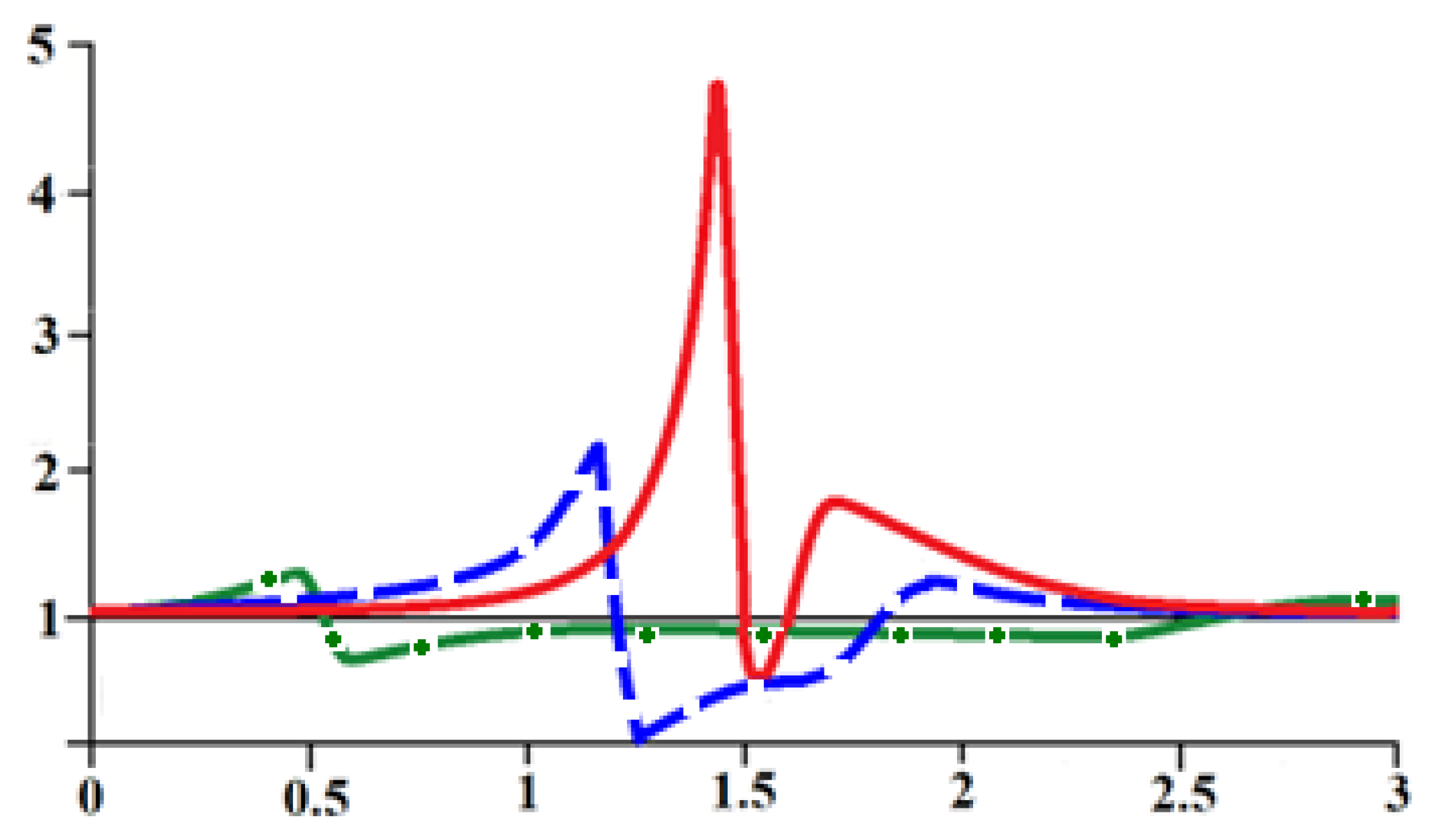
When and are well separated, i.e., , then , and . The fact that the amplitude in the K-method can be presented as a sum of the BW functions is often taken as the justification that the K-matrix pole parameters are close to those of the physical resonances. However, ‘good separation’ is a rather subjective argument; the unitarity of the S-matrix is very crudely violated, even when resonances are well spaced, as shown in Figure 1.
2. Brief Description of the Unitary BW Method
Here, we briefly describe the method of constructing the unitary S-matrix [7]. The regular procedure is presented in Appendix A.
The unitarity condition, , with , gives
The unitarization procedure becomes technically simpler if, following the idea of works [2,3], to introduce complex vectors of partial widths, . With , , , the S-matrix is:
and the T-matrix is:
Here, are energy-independent phases; factors are introduced to keep vectors dimensionless. Expression (19) is time-invariant.
The decay branching ratio of a resonance r in channel is
The partial widths are . The total and partial widths can depend on energy, .
Formulas in the rest of this section become technically simpler if the variable E is used rather than —all the expressions and algorithms can be rewritten in terms of . For
let us formulate the conditions that should be imposed on vectors to maintain unitarity. From Equation (18) we have
where the following notation is used:
The constraints Equation (23) involves complicated non-linear conditions. To resolve them, we use a method which allows substantial technical difficulties to be overcome; these previously restricted the approach to a maximum of two [3], or three [8] resonances, even when . The method is based on the construction of vectors in such a form that their imaginary parts are combinations of their real parts : , or
U is a real anti-symmetric matrix which has a simple form for any particular N and M (see Appendix A). Next, instead of trying to find all components of vectors , we only find their real parts, and then obtain their imaginary parts using matrix U. Notice that the number of free parameters, , is the same as in the K-matrix method.
When , the matrix elements and vectors become real and orthogonal, , and we return to a simple sum of the BW functions without relative phases.
The constraints on vectors are the following:
Constant coefficients are determined via the elements of matrix U.
The widths are given by Equation (26):
Formulas (25)–(29) provide the algorithm for the method. For any particular case, , , etc.; the coefficients are given by simple expressions, presented in Appendix A.
In the case of one resonance, this approach reduces to the traditional BW function:
Vector is real, and . With Equation (29), it gives the analogue of Flatte’s formula:
or in variable s,
In a fitting procedure, the free parameters are: mass and the components of vector .
If a resonance is lying above all the thresholds, its mass is simply and its width is
If a resonance is lying between the thresholds L and , there are two options: to set in the energy region below the corresponding threshold, , or to continue it as ( can take the values to consider different Riemann sheets). The effective mass is then
and the width is
For the case of two resonances and one channel, this algorithm leads to the same expression for the amplitude T as in the K-matrix method (as in Section 1).
Let us illustrate the method with the example of two resonances and two channels, , . The goal is to find vectors .
For two channels, matrix U is
( is the real parameter, ), i.e.,
The coefficients in the unitary constraint Equations (26)–(28) are:
Six real quantities, for example, masses and , parameter , and , , can be taken as independent parameters in data fitting. The remaining real component is determined from Equations (27) and (28).
When both resonances lie above the 2nd threshold, ,
After this, the components can be calculated with Equation (37). This completes the construction of the amplitudes
The functions are given by expression (29), their values at ,
can be considered as resonance “widths”.
If the 2nd threshold is located between and , i.e., , the mass of the 1st resonance, , is determined by the zero of the real part of the denominator in the first term in Equation (40), i.e., by the root of the equation
so this resonance width is
The component can be found from Equation (39) with instead of .
3. Examples: K-Matrix vs. Unitary BW Approach
Let us consider two resonances in two channels, , where is a diagonal matrix. In the unitary BW expression,
there are six independent parameters: . (The product ).
The K-matrix pole terms in expression (10),
have the same number of independent parameters: , , and two (with being normalized, ). The K-matrix amplitudes are
where .
Let us start with the important observation that the K-matrix amplitudes become zero (or are very close to zero values) between the and locations. This feature directly follows from expression (7), it is, therefore, retained in any modification of the K-matrix approach. In the case of two resonances, equation (i.e., ) is a linear equation; in the case of three states, it is a quadratic equation—these results directly follow from expressions (10) and (46). The zeros in amplitudes and are slightly shifted from the zero position in . Thus, resonances in scattering amplitudes are, in fact, well spaced (a polynomial added to expression (10) for does not change this observation, see Appendix B). As a result, this method can work well only when describing experimental data with sufficiently well-separated states.
Since the purpose of this article is to demonstrate the features of the two methods, it is more useful to consider simple examples than discuss a real physical problem in which there are always ambiguous questions, such as the choice of the most significant channels, the number of resonances, etc. Particular physical problems are beyond the scope of this paper and will be studied separately.
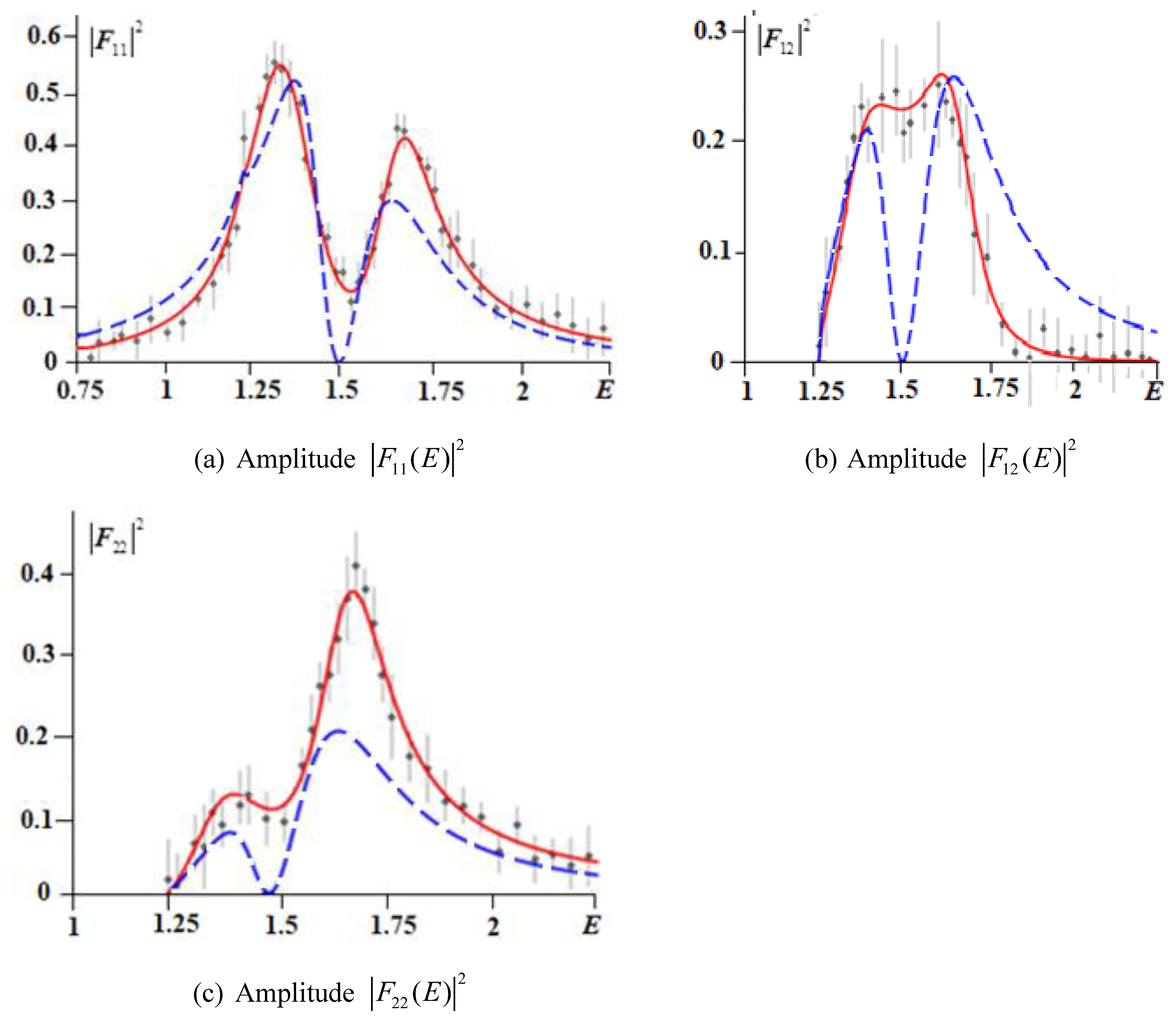
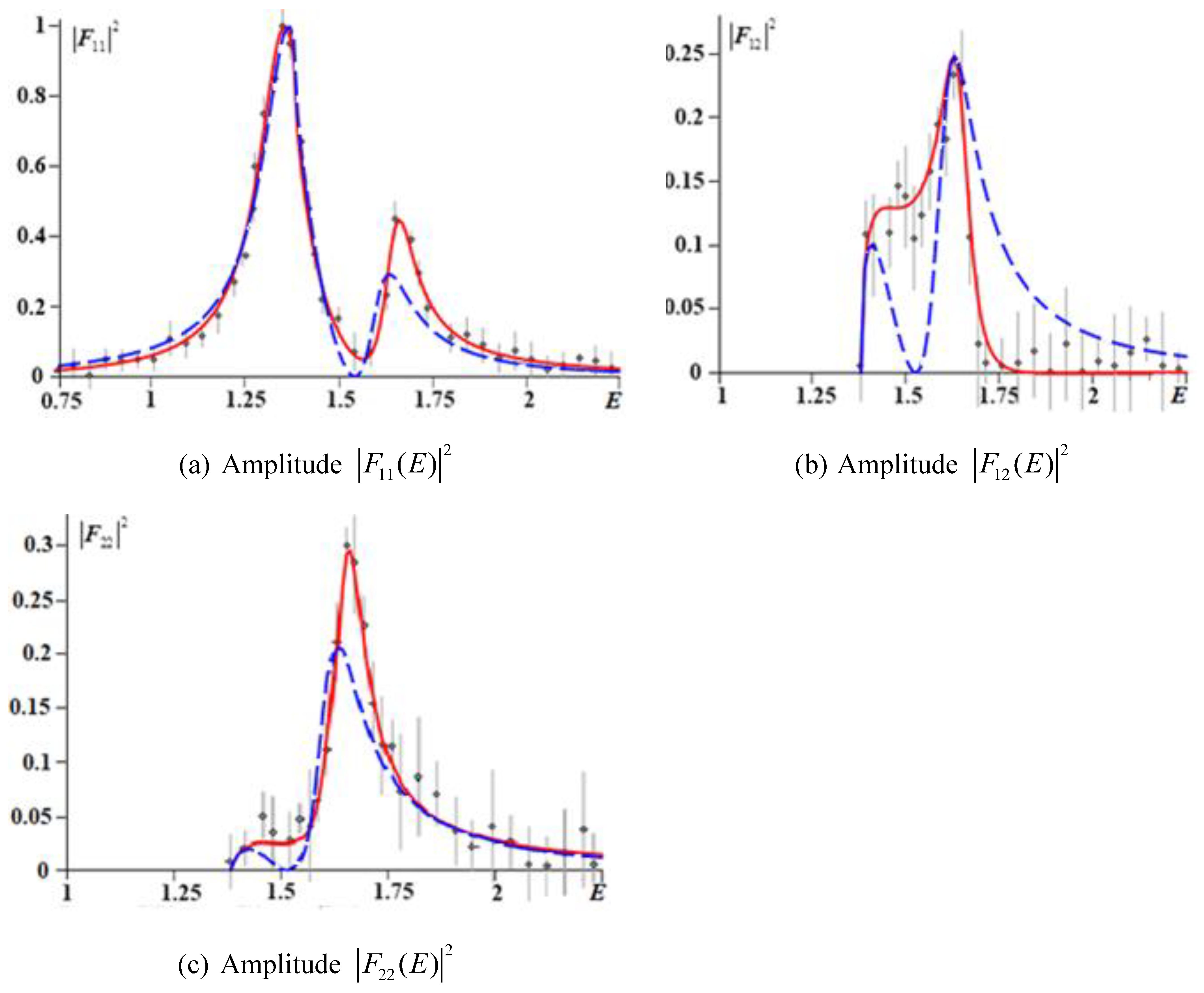
Let us start by considering two overlapping states (peaks) in the amplitudes located near and GeV, with widths about GeV. We also consider different positions of the 2nd channel threshold: below both states, at , and between the states, at (the position of the 1st threshold is fixed at ; all quantities here and below are in GeV). Next, we generate “data” which qualitatively correspond to these situations—the details about such data generation are given in Appendix B. (Note that these data are similar to the data on scattering amplitudes in the case of vector resonances.) To do this, we draw smooth curves (different peak heights and widths can be considered), then discretize and randomize these curves and introduce dispersions (error bars at each point are generated randomly with the upper limit of 0.05). Examples of such data are presented in Figure 2 for and Figure 3 for . The peaks overlap and, at least in one channel, are not well resolved, as often occurs in real situations. We then fit these data with the unitary BW formulas (44)—red lines, and K-matrix (46)—blue lines.
In calculations, we use the phase factors (these can be modified by including the barrier factors). The continuation below the threshold can be used in expression (32) for the amplitudes .
In the unitary BW formula (44) for the threshold at , the values of the six independent parameters are:
the fit gives ( is degrees of freedom number).
For the threshold at , the values of these parameters are:
the fit gives . The remaining parameters can be calculated using the six independent parameters. (After the values are found, the value of a ‘technical’ parameter is no longer required.)
Table 1 shows the BW resonance parameters—the branching ratios are calculated with formula (21), the phases can be obtained from the values, and . By the direct substitution of these in formula (44), it can be confirmed that matrix is unitary for any E.
The fit based on the K-matrix formula (46) for the threshold , gives the following values for the six independent parameters:
resulting in .
For the threshold , the parameters are:
resulting in .
Table 2 contains the K-matrix parameters. The branching ratios are .
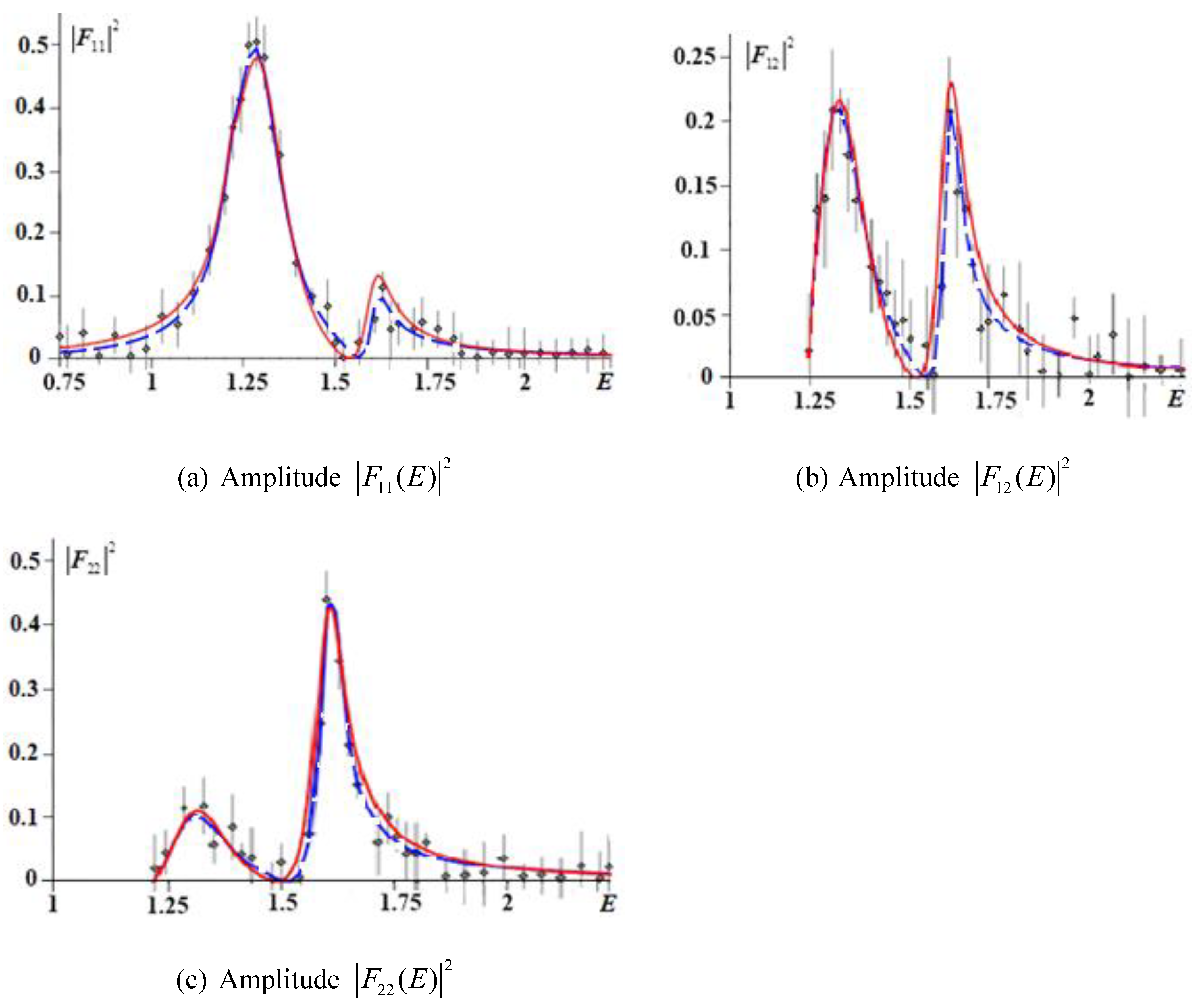
Large values of reflect the fact that the K-matrix method cannot adequately describe the data in situations when wide resonances are not well spaced, such as in the channel , in Figure 2 and Figure 3. However, this method works perfectly well when resonances are well resolved, such as in Figure 4, where the data have substantial dips between the resonances in all three channels (here, for brevity, we consider only one threshold location, ). The quality of the fits in both methods is practically the same, . The resonance parameters for Figure 4 are shown in Table 3.
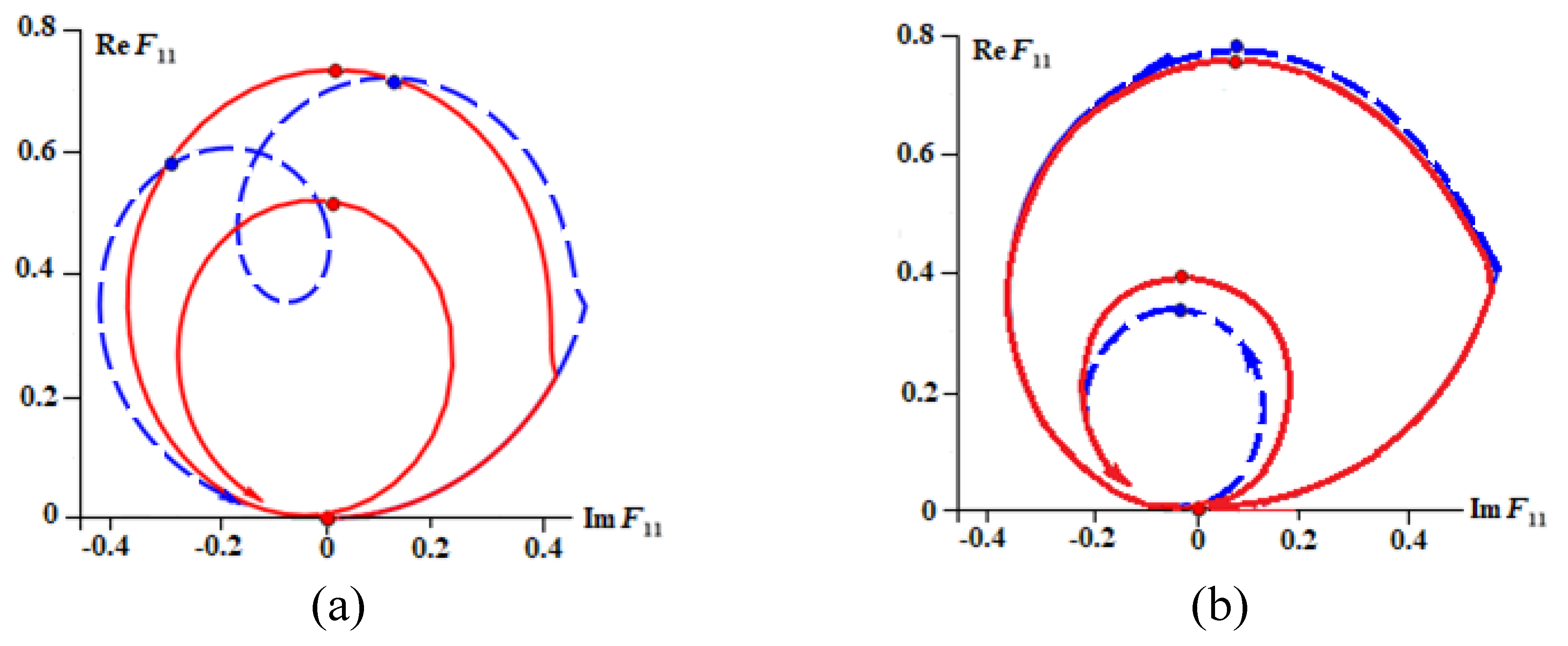
The Argand diagrams corresponding to the amplitude in Figure 2 and Figure 4 are shown in Figure 5.
4. Background
Taking background into account in a rigorous way is especially important when several resonances are not well resolved, or their existence is not well established. Even a small background can hide a resonance [9,10], as in the situation with a vector meson overlapping with other wide vector states, and .
Usually, to account for the background in the K-matrix description, polynomials are added to the pole terms in :
The form (47) does not allow the background to be presented in terms of background phases, ; in this form, here, even the number of parameters is different to that in (47): for example, for two channels and an energy-independent background, there are two parameters and , versus three in . Thus, polynomials in Equation (47) only allow the use of additional fitting parameters besides the pole parameters.
Another important fact is that the K-matrix resonances remain well spaced even when polynomials in are taken into account; for details see Appendix B.
In the BW scheme, the S-matrix can be separated in a sum of the resonant and background terms from the very beginning:
The unitary and symmetric background matrix B can be constructed as described below.
If matrix B is diagonal, i.e., it is non-zero only in channels with ,
vectors in (48) can be presented as
where can be found with the procedure described in the previous sections. Matrix S, in such a situation, is
or
If matrix B is non-diagonal, i.e., a background potentially is not zero in all channels, it is helpful to present it in form [3], , where W is a real orthogonal matrix, and is a diagonal matrix ( when matrix B is diagonal). Writing matrix B as with we define ; thus, and matrix S can be expressed as , where does not contain a background:
Obviously, is unitary if matrix is unitary. Therefore, we can independently find vectors in , and then return to the matrix .
Matrix W can be constructed as a sequence of rotations:
Matrix is convenient to write in the form:
; here are the rotation angles.
For instance, for three channels
where
The quantities , can be taken as fitting parameters (they can be functions of energy).
We, then, have
with the matrix
Thus, the background in the unitary BW method can be described by formulas (54) and (55).
To demonstrate this scheme, let us take the case of two resonances and three channels using the resonance parameters in Table 4.
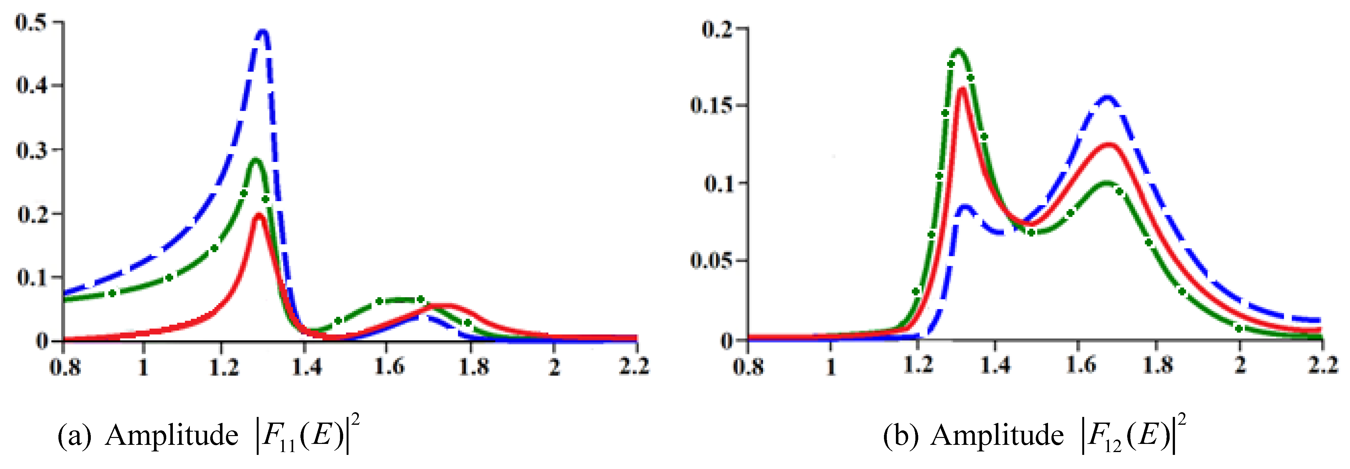
Next, we include a background in these resonant unitary BW amplitudes to see how it modifies the scattering amplitudes. In Figure 6, graphs of and (chosen as examples) are shown for the cases of diagonal and non-diagonal backgrounds. The assigned background parameters (the choice of these values is determined only for the purpose of illustrating the complex role of the background in the scattering amplitudes) are listed in the Figure 6 caption. For brevity, we use an energy-independent background.
It is seen that even a small diagonal background modifies the resonance shapes. The non-diagonal background affects even the peak locations. For example, the second peak in is shifted by about 0.15 from , the “correct” one. Since a background contribution may be very different to the intuitively expected smooth plateau in each of the channels, an adequate treatment of the background is absolutely necessary when describing overlapping multichannel states.
Because a priori there are no criteria for choosing the background parametrization, an additional uncertainty to resonance parameters is added. If some particular parametrization fits the data substantially better than the others, it can be considered as a practical criterion. If this is not the case, then a simplified approach may be the following: first, evaluate the background by smoothing (“smearing”) the data [11,12]—this procedure will remove all the peaks; then, subtract the background obtained in this way from the data and analyze the remainder using methods that preserve unitarity—a similar approach was used in work [13] to analyze overlapping and resonances (in the approximation of constant widths).
5. Conclusions
The parameters of broad inelastic resonances depend on the way the scattering data are analyzed. Obviously, the interference between resonances is the central part of an analysis and interpretation. In this respect, the usual Breit–Wigner parametrization which does not satisfy unitarity, is very unreliable (as shown in Figure 1); for example, it can possibly lead to deviations in mass of more than 100 MeV in the case of mesons [14].
There are different unitarization techniques to describe resonant states, both theoretical and phenomenological. Many analyses describe multi-channel resonances as poles on unphysical Riemann sheets for scattering amplitudes, as in works [10,15]. Resonances can be given by poles and corresponding zeros on an uniformization plane, which allows the description of broad multi-channel resonances [16]. The inverse amplitude method is another unitarization technique to present resonances and to enlarge the energy applicability region of effective Lagrangians [17].
We compare the results of the unitary BW approach and the standard widely used K-matrix method [5]. Both methods lead to similar results when resonances in all channels are well resolved, with a better ability of the BW method to resolve wide overlapping resonances. Another advantage of the BW method is that scattering amplitudes can be separated in the resonant and background contributions. A background, in terms of the phase shifts, does not necessarily form a smooth plateau in scattering amplitudes, and its adequate treatment is critically important for describing overlapping multichannel states.
Papers on overlapping resonances often include statements that because a sum of the BW functions violates the unitarity, a BW description cannot be used by default. Here, we draw attention to the fact that the unitary BW form for several states is possible when the BW functions are taken with the proper phase factors. From a theoretical point of view, it worth knowing that the problem formulated a long time ago [2], to present the unitary S-matrix as a sum of BW terms, has a regular solution. This approach can be used in fitting procedures, along with the K-matrix and other methods. Despite the K-matrix description being perfectly adequate as unitary parametrization for relatively narrow resonances, the names of its parameters, e.g., “masses”, “widths”, “and branching ratios” are only borrowed from the BW description through the comparison with a single resonance situation. A unitary BW model-independent method to describe overlapping resonances, with the parameters having direct physical meaning and the background being treated in a regular quantum mechanics form [18], can be a good addition to other unitarization techniques.
Author Contributions
V.H.–theory; T.B.–calculations. All authors have read and agreed to the published version of the manuscript.
Funding
This research received no external funding.
Data Availability Statement
The data is available upon request from authors.
Conflicts of Interest
Authors declare no conflict of interest.
Appendix A. Construction of Unitary S Matrix in BW Approach
Despite the formulas below looking somewhat sophisticated, their final form for a particular num;ber of channels and states is rather simple.
For N resonances and M channels, the S matrix is given by (background contribution is considered in Section 4) the expression
with (variable E is used only to simplify the formulas)
The unitarity condition gives
or
where
Multiplying Equation (A3) by the product , we obtain
with , .
To satisfy the unitarity relation (A3), it is necessary and sufficient that coefficients of the polynomial (A5) be zero for all powers of . The coefficient of is
Here, and are coefficients at the powers in the polynomials and , respectively.
Equating the coefficient to zero at the highest degree , taking into account that is the polynomial of degree and is the polynomial of degree we obtain:
where , .
The key moment of the method is that we construct the imaginary parts of vectors as linear combinations of their real parts ():
Substituting expression (A8) into relation (A7), we obtain and ; thus, U is an anti-symmetric matrix. (If there is no time-reversal symmetry restriction, matrix U can take a more general form, not necessarily anti-symmetric.) Equation (A8) gives NM relations involving parameters (matrix elements ).
Next, equate the coefficient to zero at :
Because we obtain
Taking into account expression (A8), we can state
In order for the coefficient in (A10) at to be zero, it is necessary to set the coefficients of all products to zero, . We substitute expressions (A11) into relation (A10) and equate the real and imaginary parts of these coefficients to zero. This yields:
Thus, we obtain simultaneous equations linear in the scalar products , and : N equations (A12), equations (A13), and equations (A14). The coefficients at and are identical because equations (A13) and (A14) are symmetrical under the and interchange.
Solving these equations, we obtain (recall that ):
where
Here,
is the minor with the rows and the columns of matrix U . Notations such as mean an integer part of the expression in the brackets.
Relations (A8) and the scalar products (A15) completely define the conditions imposed on vectors . It can be shown that if vectors satisfy the relations (A8) and (A15), then the coefficients at lower degrees of polynomial (A5) are identically equal to zero.
For practical purposes, it is convenient to express the scalar products (A15) in terms of real vectors :
The domain of the elements of the matrix U is defined by the conditions
which follows from the Cauchy–Schwarz inequality .
It is seen from these inequalities that if resonances are very far from each other, then and vectors become real and orthogonal. In this situation, the lengths of vectors are equal to the resonance widths , but, in general, these lengths are larger than :
There is also a sum rule for vectors :
The branching ratios for the decay of the r-th resonance in the i-th channel is
For , we have:
where and are real phases of vectors and , .
In a potential fitting procedure there are real parameters: ,, . Besides these, the relations (A15) contain elements of real anti-symmetric matrix U (These are ‘technical’ and do not appear in the final expression for the S-matrix.) Not all these parameters are independent. The relations (A6) connect the real and imaginary parts of vectors . Moreover, the real parts, , are connected by relations (A15). Thus, in total there are free real parameters:
the same number as in the K-matrix parametrization.
Even though the formulas (A15) look somewhat sophisticated, the resonance parameters can be determined using a straightforward regular algorithm; the unitarity of S can be confirmed at every value of E. In this Appendix, we use the energy variable E to avoid unnecessary complications in the formulas; however, the algorithm can be rewritten in terms of the variable , as in Section 1 and in one of the Examples in Section 3.
For two resonances, the algorithm is presented in the main text.
For three resonances, , matrix S(E) is
Matrix U, relating the real and imaginary parts of vectors , , , is
i.e.,
Real parameters are restricted by the relation
The coefficients in formulas (A16) are:
Substituting these in formulas (A16), we obtain the relations needed to construct vectors , and :
The widths are
where are zeros of real parts of denominators in the corresponding BW terms.
Let us very briefly describe the case of four resonances, . Matrix U is
thus,
The lengths of vectors , , , and the angles between them are determined by the scalar products (A15) for . From that we have for the coefficients in formulas (A16):
where
Formulas (A15) give the scalar products—as an example we present two of these here:
Appendix B. K-Matrix Interactive Software Description
We created an interactive software to work with K-matrix scattering amplitudes , which helps to see the main features of this method. This Appendix contains its brief description. This software can be provided upon request to interested colleagues.
The feature which directly follows from (A26) and (A27) is that resonance peaks in are well resolved, the scattering amplitudes have zero, or very close to zero, values between the pole locations . (The introduction of Adler’s zero in expression (A27) does not change this feature.) For instance, in the case of two resonances, the zero of equation (i.e., ) is located between the poles and , and is given by a linear equation; in the case of three states, this is given by a quadratic equation. The zeros in and are slightly shifted from zero. In general, for , when a polynomial contribution in (A27) is substantial, instead of exact zeros, there are deep minima in between the peaks—the resonances in the K-matrix method are always well separated.
This particular software has three sections:
(a)
two channels, two resonances;
(b)
two channels, three resonances;
(c)
three channels, two resonances.
The phase factors are:
, where ; the resonances lie above the opening threshold, i.e.,.
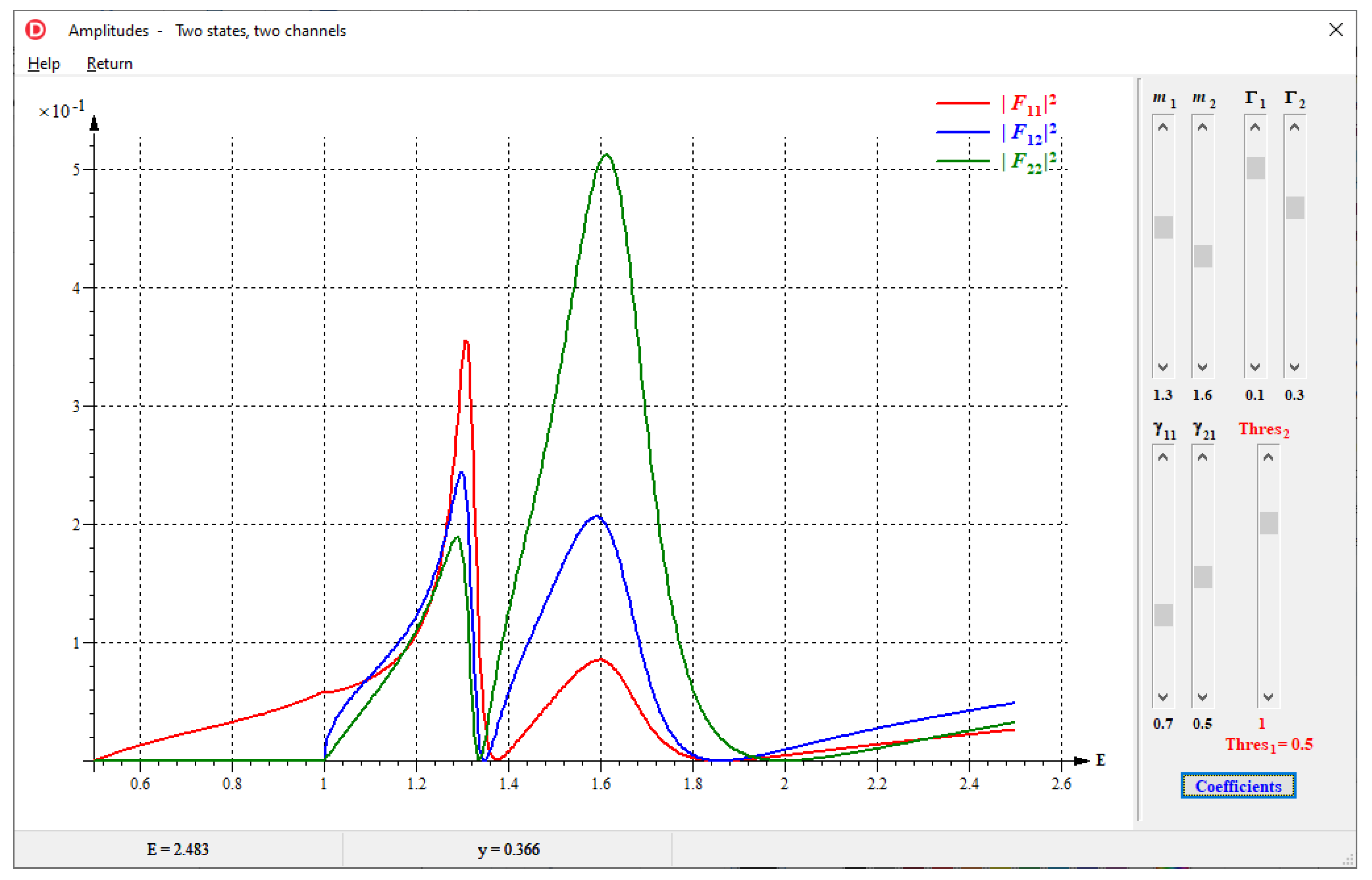
Appendix B.1. Two States, Two Channels
In the case of two channels, matrix T is:
where .
So
For two poles in , the independent parameters are: six in the pole terms (their values can be set by using the interface scroll bars):
and six coefficients (their values can be entered interactively).
An obvious restriction on polynomial coefficients is that resonance peaks should not be wiped out.
Example
Enter the polynomial coefficients in the Table:
Set the poles parameters and the threshold positions, and by using scroll bars—see the screenshot in Figure A1:
The parameters in the screenshot in Figure A1 are:
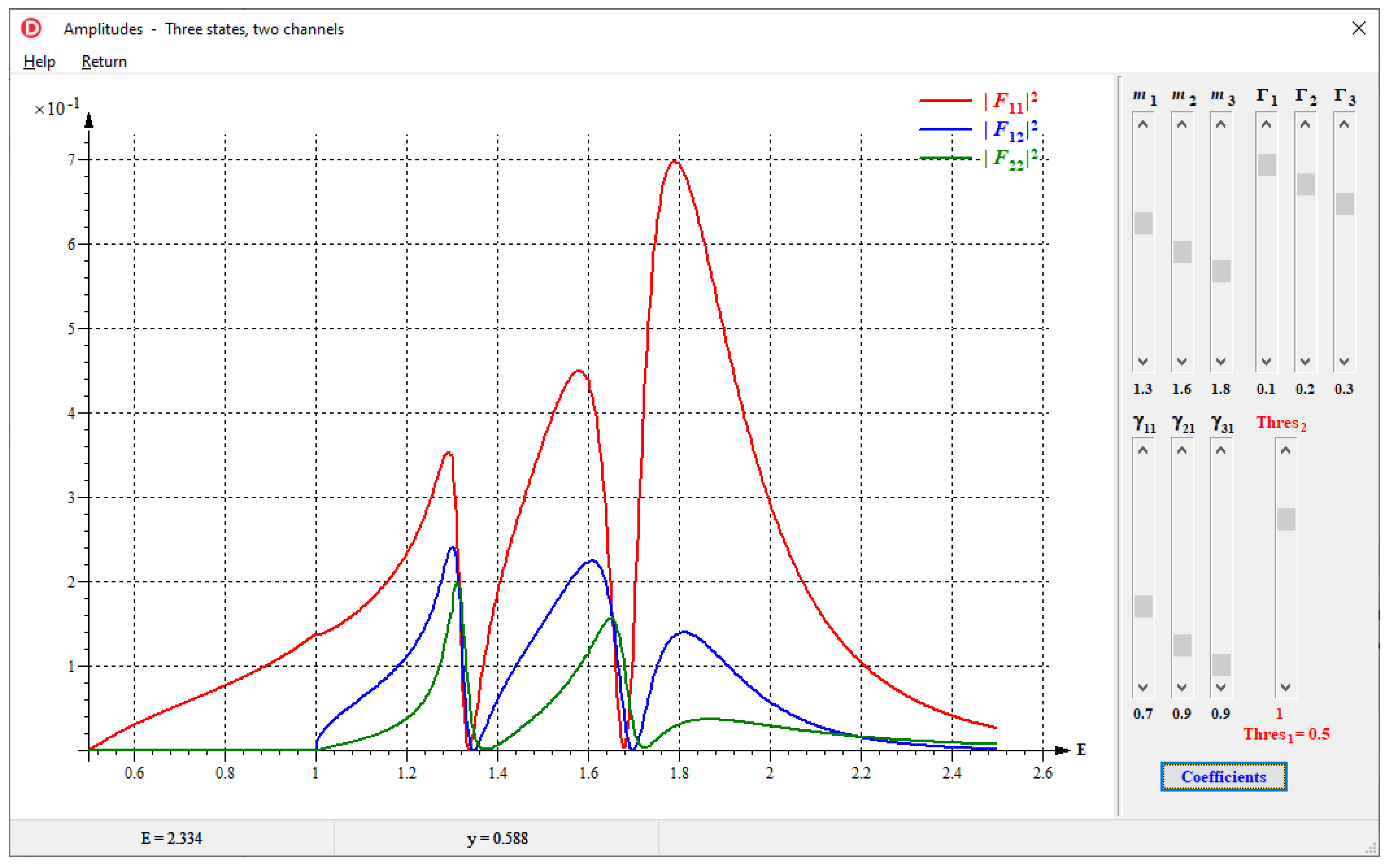
Appendix B.2. Three States, Two Channels
For three poles and two channels, the independent parameters are:
Example
Enter the polynomial coefficients in the Table:
Set the poles parameters and the threshold positions, and by using scroll bars—see the screenshot in Figure A2:
The parameters in the screenshot in Figure A2 are:
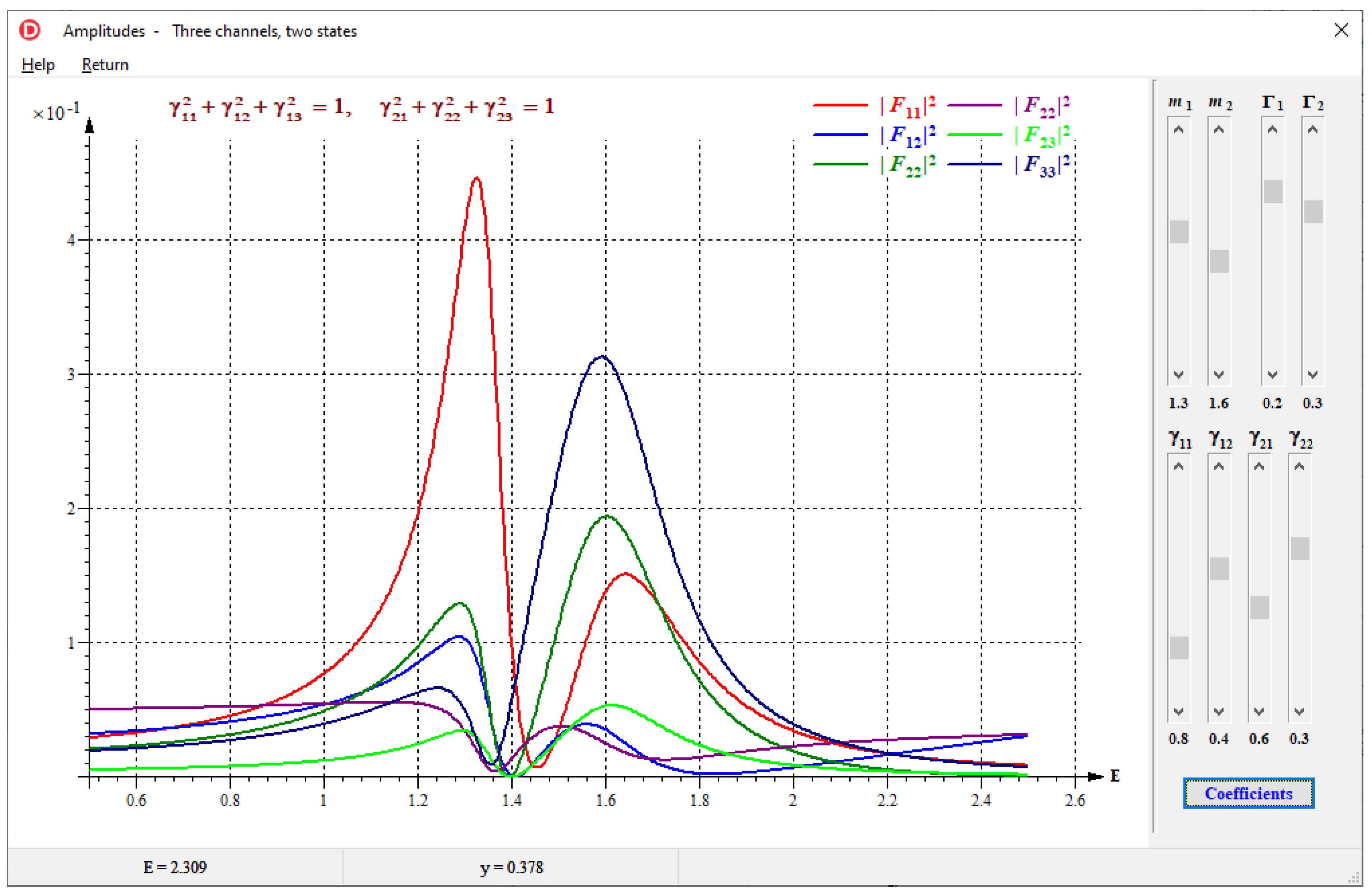
Appendix B.3. Three Channels, Two States
(In this part of the software, in order do not overcomplicate the interface, we take .)
The eight independent parameters are:
( is normalized, ).
Example
Enter the polynomial coefficients in the Table:
Set the poles parameters by using scroll bars—see the screenshot in Figure A3:
The parameters in the screenshot in Figure A3 are:
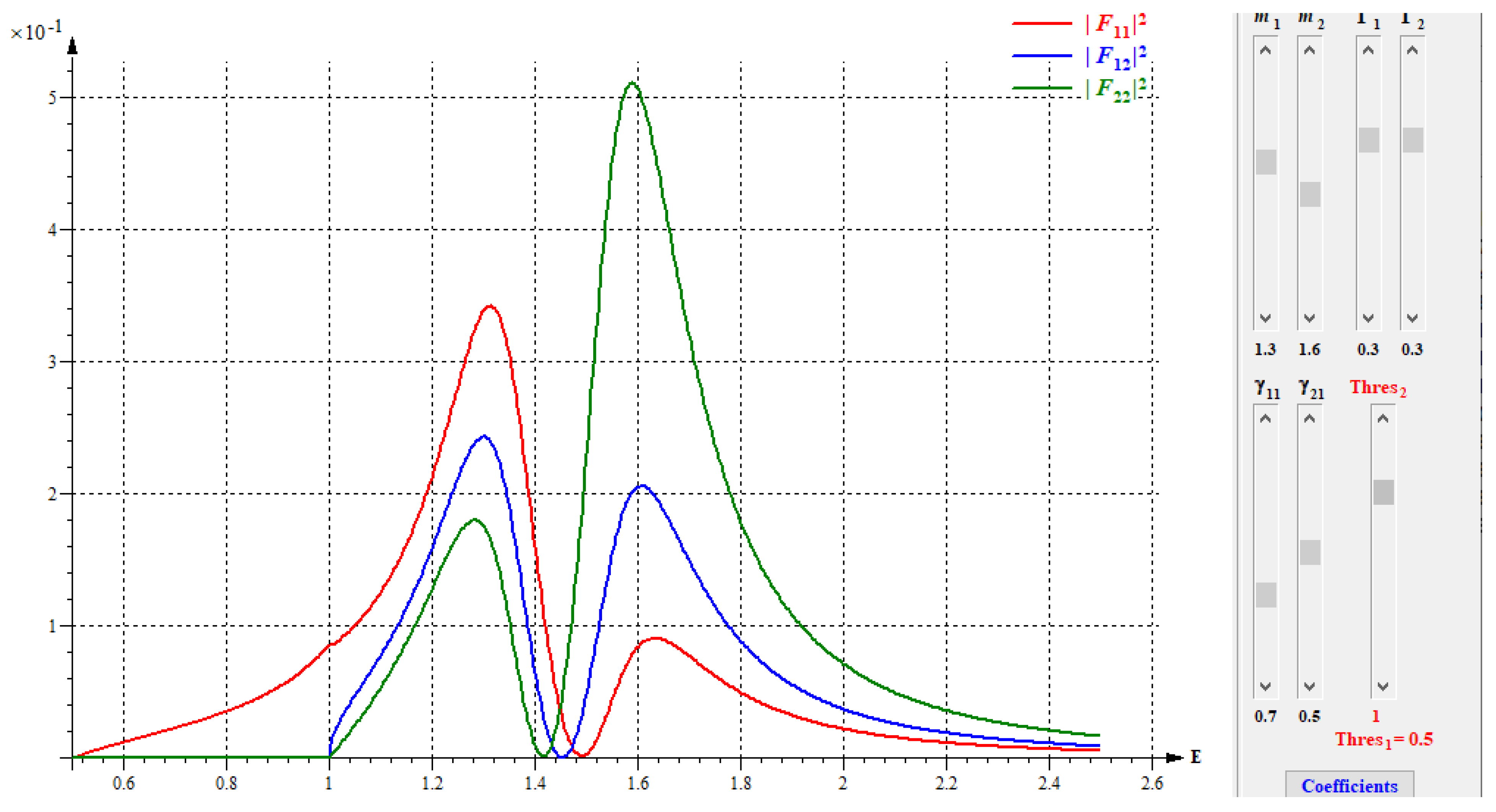
The purpose of the following example is to demonstrate that the K-matrix amplitudes can be always fitted with the unitary BW method, but the opposite is not true if amplitudes in all channels do not have zeros between resonance peaks, in other words, when the peaks actually overlap.
Consider the K-matrix amplitudes in the screen-shot in Figure A4.
The values of the K-matrix parameters in the screenshot in Figure A4 are:
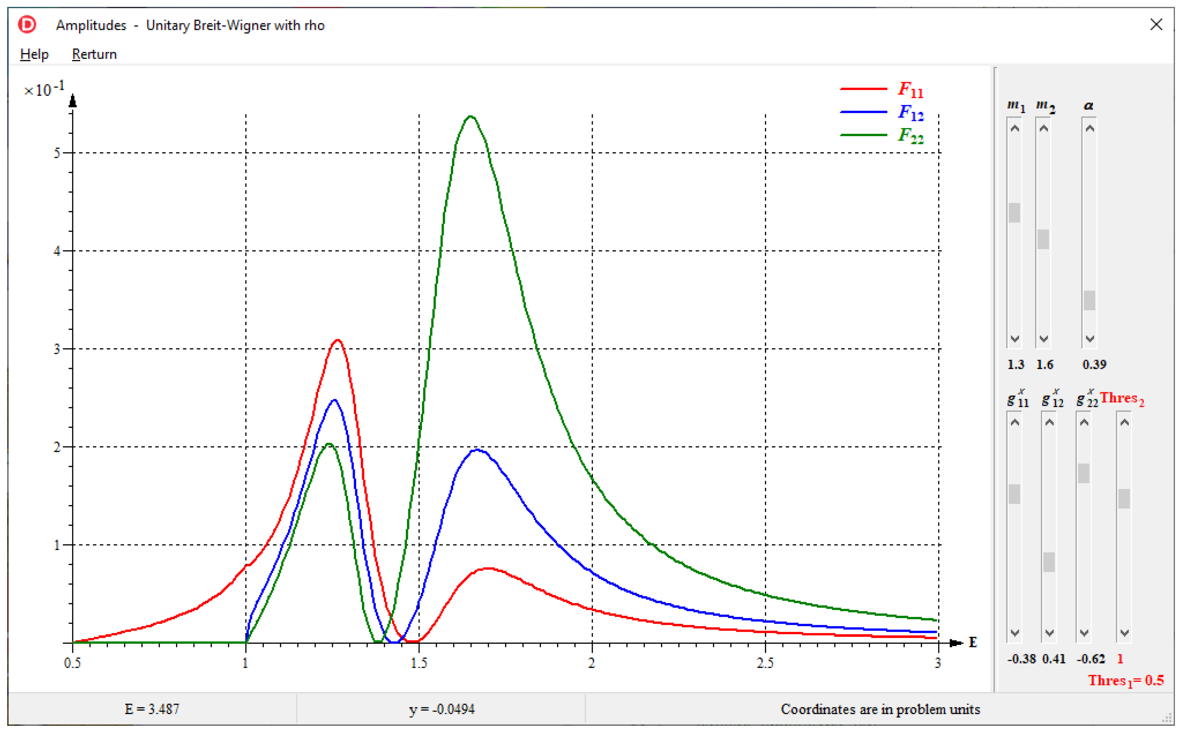
Then we do the fit to these K-matrix curves by using the unitary BW formulas. In the first step we use the BW software to obtain qualitatively similar result to the K-matrix curves. The results of this first step (a visual approximation) are shown in Figure A5 (BW software screenshot).
The values of the BW parameters (entered with scroll-bars) in the screenshot in Figure A5 are:
It gives the following BW physical parameters:
Branching ratios
BW widths
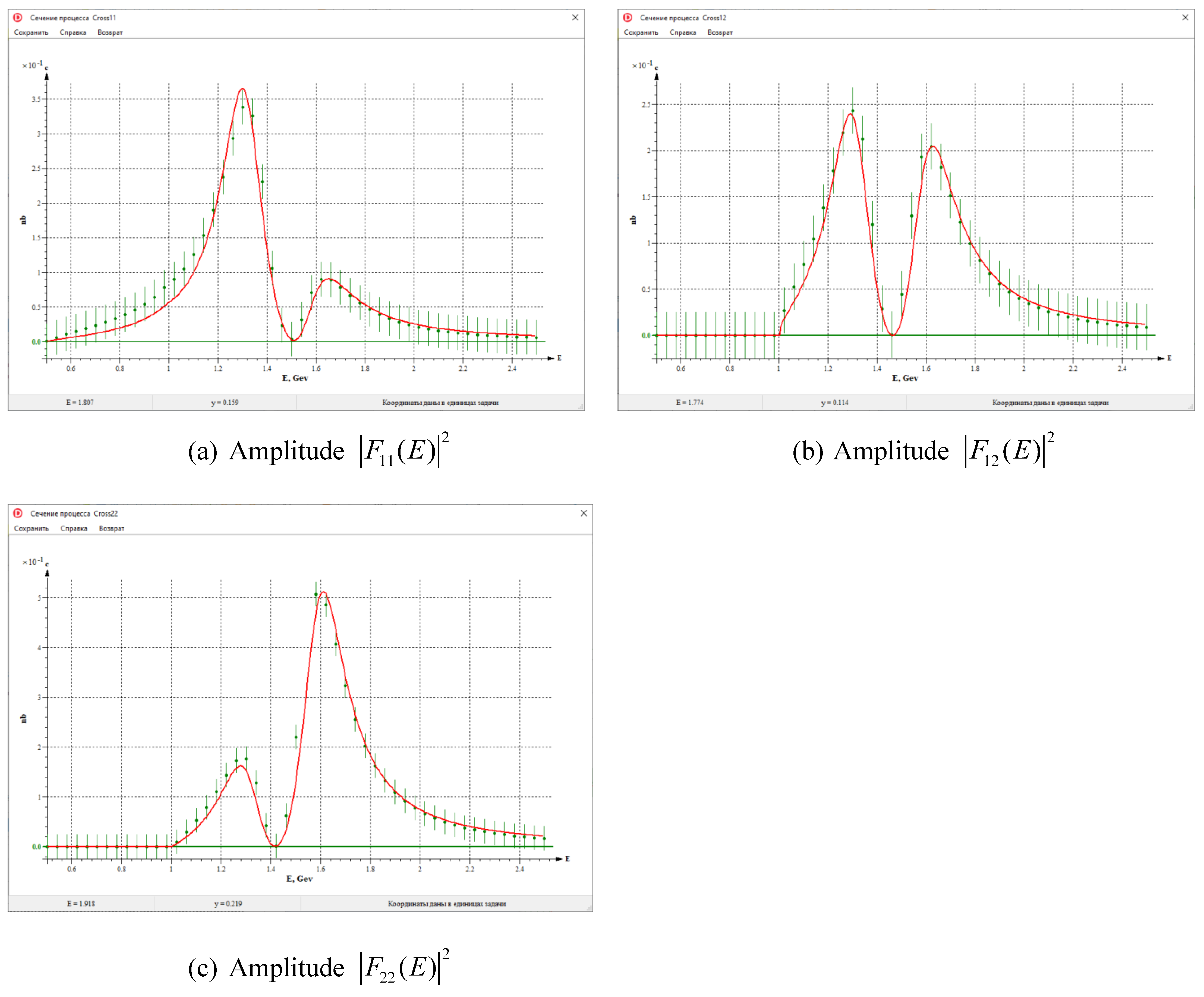
After that preliminary step (which is not compulsory but helpful) we do fitting to the K-matrix curves for a more accurate finding of BW parameter values.
Appendix B.4. Fitting to K-Matrix Curves Using the Unitary BW Formulas
“Experimental points” represent the K-matrix curves – emphasize that this is a 100% bias situation for the K-matrix method. The result of the fitting is shown in Figure A6. (Technically, to do fitting we assign error bars.)
With the error bar shown in the Figures, (this value is taken arbitrarily—it affects only the value of ), , .
Therefore, the data which can be successfully fitted with the K-matrix method, can also be fitted with the unitary BW approach. Both methods lead to similar results when resonances in all channels are well resolved. However, the opposite is not true if amplitudes in all channels do not have zeros between resonance peaks; in other words, when the peaks actually overlap. Such a case is shown in Figure A7 (BW software screenshot)—the amplitudes, chosen simply as an example, cannot be fitted with the K-matrix approach with any reasonable value of the
Clearly, there could be data for which both methods cannot give good fitting results for all channels scattering amplitudes; technically, this is related to insufficient number of fitting parameters to describe all , . (Obviously, when the data for some channels are missing, as often occurs, the fitting task is much easier.) Physically, poor fitting may be a signal of incompleteness or incompatibility of data.
Humblet, J.; Rosenfeld, L. Theory of nuclear reactions: I. Resonant states and collision matrix. Nucl. Phys.1961, 26, 529. [Google Scholar] [CrossRef]
McVoy, K.W. Overlapping resonances and S-matrix unitarity. Ann Phys.1969, 54, 552. [Google Scholar] [CrossRef]
Dalitz, R.H. On the strong interactions of the strange particles. Rev. Mod. Phys.1961, 33, 471. [Google Scholar] [CrossRef]
Chung, S.U.; Brose, J.; Hackmann, R.; Klempt, E.; Spanier, S.; Strassburger, C. Partial wave analysis in K-matrix formalism. Ann. Phys.1995, 4, 404. [Google Scholar] [CrossRef]
Aitchison, I.J.R. The K-matrix formalism for overlapping resonances. Nucl. Phys. A1972, 189, 417. [Google Scholar] [CrossRef]
Henner, V.K.; Belozerova, T.S. Analysis of overlapping resonances using the K-matrix and Breit-Wigner method. Phys. Part. Nucl.2020, 51, 673. [Google Scholar] [CrossRef]
Durand, L. S-matrix treatment of many overlapping resonances. Phys. Rev. D1976, 14, 3174. [Google Scholar] [CrossRef]
Henner, V.K. Why is the not observed in the scattering? Z. Phys. C1985, 29, 107. [Google Scholar]
Hammoud, N.; Kaminski, R.; Nazari, V.; Rupp, G. Strong evidence of from a unitary multichannel reanalysis of elastic scattering data with crossing-symmetry constraints. Phys. Rev. D2020, 102, 054029. [Google Scholar]
Poggio, E.C.; Quinn, H.R.; Weinberg, S. Smearing method in the quark model. Phys. Rev. D1976, 13, 1958. [Google Scholar]
Henner, V.K.; Frick, P.G.; Belozerova, T.S. Application of wavelet analysis to the spectrum of states and the ratio . Eur. Phys. J. C2002, 26, 3. [Google Scholar]
Henner, V.K.; Davis, C.L.; Belozerova, T.S. Using wavelet analysis to compare the QCD prediction and experimental data on and to determine parameters of the charmonium states above the threshold. Eur. Phys. J. C2015, 75, 509. [Google Scholar]
Bartos, E.; Dubnicka, S.; Liptaj, A.; Dubnickova, A.Z.; Kaminski, R. What are the correct meson mass and width values? Phys. Rev. D2017, 96, 113004. [Google Scholar]
Bydžovský, P.; Kamiński, R.; Nazari, V. Modelling ππ amplitudes with σ poles. Phys. Rev. D2014, 90, 116005. [Google Scholar]
Surovtsev, Y.S.; Bydžovský, P.; Lyubovitskij, V.E. Nature of the scalar-isoscalar mesons in the uniformizing-variable method based on analyticity and unitarity. Phys. Rev. D2012, 85, 036002. [Google Scholar]
Nicola, A.G.; Peláez, J.R.; Ríos, G. Inverse amplitude method and Adler zeros. Phys. Rev. D2008, 77, 056006. [Google Scholar]
Figure 1.
Plot of for a sum of two BW functions. Green dashed-dotted line , , , ; blue dashed line , , , ; red solid line , , , (all in GeV).
Figure 1.
Plot of for a sum of two BW functions. Green dashed-dotted line , , , ; blue dashed line , , , ; red solid line , , , (all in GeV).
Figure 2.
Panel (a) , panel (b) , panel (c) . Red solid lines—BW formula (44); blue dashed lines—K-matrix Equation (46); threshold .
Figure 2.
Panel (a) , panel (b) , panel (c) . Red solid lines—BW formula (44); blue dashed lines—K-matrix Equation (46); threshold .
Figure 3.
Panel (a) , panel (b) , panel (c) . Red solid lines—BW formula (44), blue dashed lines—K-matrix Equation (46); threshold .
Figure 3.
Panel (a) , panel (b) , panel (c) . Red solid lines—BW formula (44), blue dashed lines—K-matrix Equation (46); threshold .
Figure 4.
Panel (a) , panel (b) , panel (c) . Red solid lines—BW formula (44), blue dashed lines–K-matrix Equation (46); threshold .
Figure 4.
Panel (a) , panel (b) , panel (c) . Red solid lines—BW formula (44), blue dashed lines–K-matrix Equation (46); threshold .
Figure 5.
Argand diagrams for the amplitude in Figure 2 (a), and in Figure 4 (b). Red solid lines-BW formula (44), blue dashed lines -K-matrix Equation (46).
Figure 5.
Argand diagrams for the amplitude in Figure 2 (a), and in Figure 4 (b). Red solid lines-BW formula (44), blue dashed lines -K-matrix Equation (46).
Figure 6.
Panel (a): . Red solid line—no background, , ; green dashed-dotted line—, ; blue dashed line—, . Panel (b): . Red solid line— (no background); green dashed-dotted line—; blue dashed line— ( do not contribute to non-diagonal amplitudes).
Figure 6.
Panel (a): . Red solid line—no background, , ; green dashed-dotted line—, ; blue dashed line—, . Panel (b): . Red solid line— (no background); green dashed-dotted line—; blue dashed line— ( do not contribute to non-diagonal amplitudes).
Figure A1.
K-matrix scattering amplitudes.
Figure A1.
K-matrix scattering amplitudes.
Figure A2.K-matrix scattering amplitudes.
Figure A2.K-matrix scattering amplitudes.
Figure A3.K-matrix scattering amplitudes.
Figure A3.K-matrix scattering amplitudes.
Figure A4.K-matrix scattering amplitudes.
Figure A4.K-matrix scattering amplitudes.
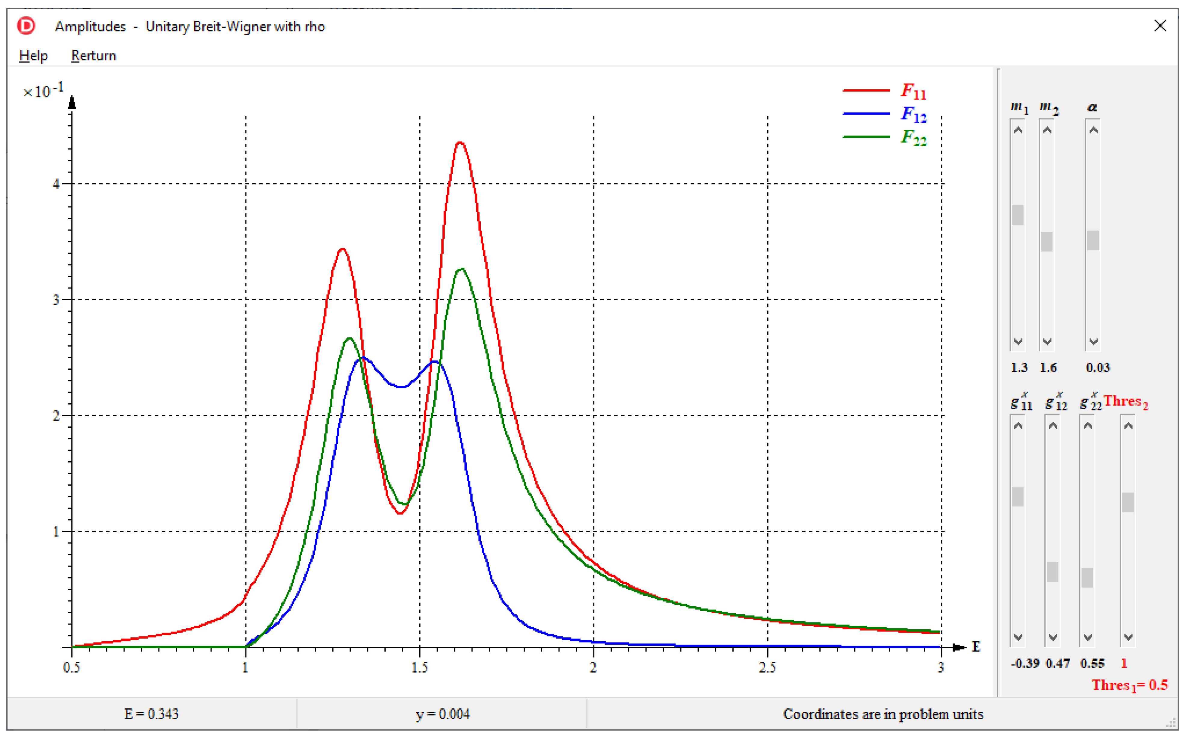
Figure A5.
Unitary BW scattering amplitudes.
Figure A5.
Unitary BW scattering amplitudes.
Figure A6.
Unitary BW scattering amplitudes.
Figure A6.
Unitary BW scattering amplitudes.
Figure A7.
Unitary BW scattering amplitudes.
Figure A7.
Unitary BW scattering amplitudes.
Table 1.
BW parameters for two threshold positions.
Table 1.
BW parameters for two threshold positions.
1.32
0.26
53
47
−0.43 − i0.03
0.41 − i0.04
1.36
0.19
55
45
−0.43 − i0.02
−0.38 − i0.03
1.65
0.318
44
56
0.43 − i0.03
0.49 + i0.03
1.65
0.14
42
58
0.30 − i0.03
0.36 − i0.03
Table 2.
K-matrix parameters for two threshold positions.
Table 2.
K-matrix parameters for two threshold positions.
1.36
0.27
59
41
1.37
0.32
54
46
1.63
0.37
47
53
1.63
0.20
40
60
Table 3.
BW and K-matrix parameters for data in Figure 4.
Table 3.
BW and K-matrix parameters for data in Figure 4.
BW
K
1.30
0.19
49
51
−0.39 − i0.02
−0.37 − i0.03
1.30
0.28
45
55
1.60
0.09
18
82
−0.11 − i0.05
−0.25 + i0.06
1.60
0.12
27
73
Table 4.
BW pole functions.
Table 4.
BW pole functions.
r
Resonance 1
1.30
0.10
40
40
20
Resonance 2
1.70
0.30
20.8
59.4
19.8
Publisher’s Note: MDPI stays neutral with regard to jurisdictional claims in published maps and institutional affiliations.
Henner, V.; Belozerova, T.
Analysis of Overlapping Resonances with Unitary Breit–Wigner and K-Matrix Approaches. Particles2022, 5, 451-487.
https://doi.org/10.3390/particles5040035
AMA Style
Henner V, Belozerova T.
Analysis of Overlapping Resonances with Unitary Breit–Wigner and K-Matrix Approaches. Particles. 2022; 5(4):451-487.
https://doi.org/10.3390/particles5040035
Chicago/Turabian Style
Henner, Victor, and Tatyana Belozerova.
2022. "Analysis of Overlapping Resonances with Unitary Breit–Wigner and K-Matrix Approaches" Particles 5, no. 4: 451-487.
https://doi.org/10.3390/particles5040035
Article Metrics
No
No
Article Access Statistics
For more information on the journal statistics, click here.
Multiple requests from the same IP address are counted as one view.
Henner, V.; Belozerova, T.
Analysis of Overlapping Resonances with Unitary Breit–Wigner and K-Matrix Approaches. Particles2022, 5, 451-487.
https://doi.org/10.3390/particles5040035
AMA Style
Henner V, Belozerova T.
Analysis of Overlapping Resonances with Unitary Breit–Wigner and K-Matrix Approaches. Particles. 2022; 5(4):451-487.
https://doi.org/10.3390/particles5040035
Chicago/Turabian Style
Henner, Victor, and Tatyana Belozerova.
2022. "Analysis of Overlapping Resonances with Unitary Breit–Wigner and K-Matrix Approaches" Particles 5, no. 4: 451-487.
https://doi.org/10.3390/particles5040035


