
Prediction of Coal Spontaneous Combustion Hazard Grades Based on Fuzzy Clustered Case-Based Reasoning

Abstract
:1. Introduction
2. Dataset Preparation
2.1. Dataset Collection
2.2. Classification of Coal Spontaneous Combustion Hazard Grades
2.3. Data PreProcessing
2.3.1. Making Data Dimensionless
2.3.2. MeanRadius-SMOTE
- (1)
- Calculate the geometric center of each class of minority class samples and represent it as .
- (2)
- Calculate the Euclidean distance from each minority class sample to the sample center and then calculate the average distance, represented as .
- (3)
- Randomly select minority class samples and obtain vectors from the sample center to the samples. Calculate the composite vector of the vector.
- (4)
- Determine the distance between the new sample and the sample center according to the average value and the parameter . Generate new samples based on Equation (2).
- (5)
- Repeat Steps 3 and 4 until the sample size of the majority and minority class is balanced.
3. Machine Learning Modelling
3.1. Overview of the Machine Learning Models
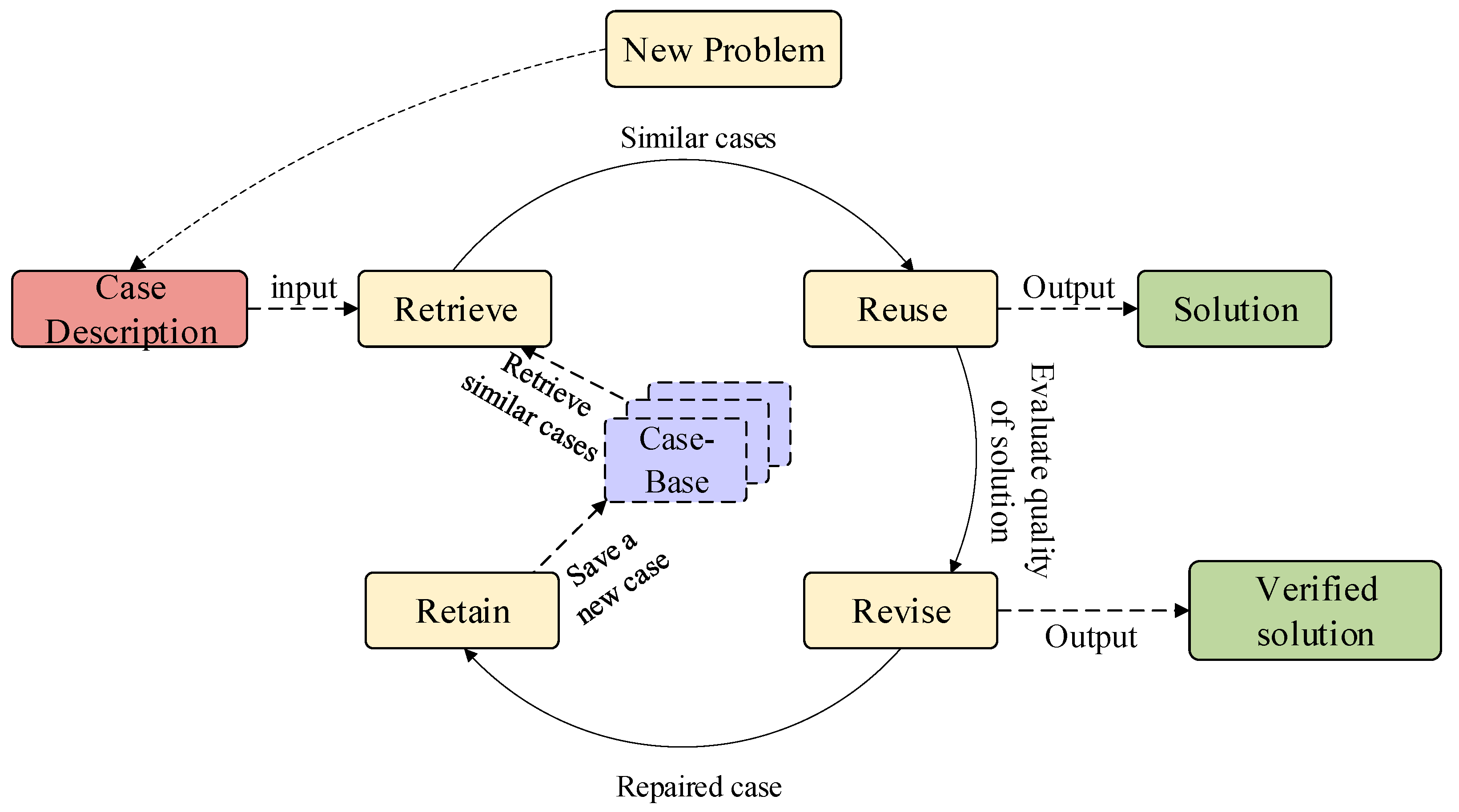
3.1.1. Case-Based Reasoning
3.1.2. FCM
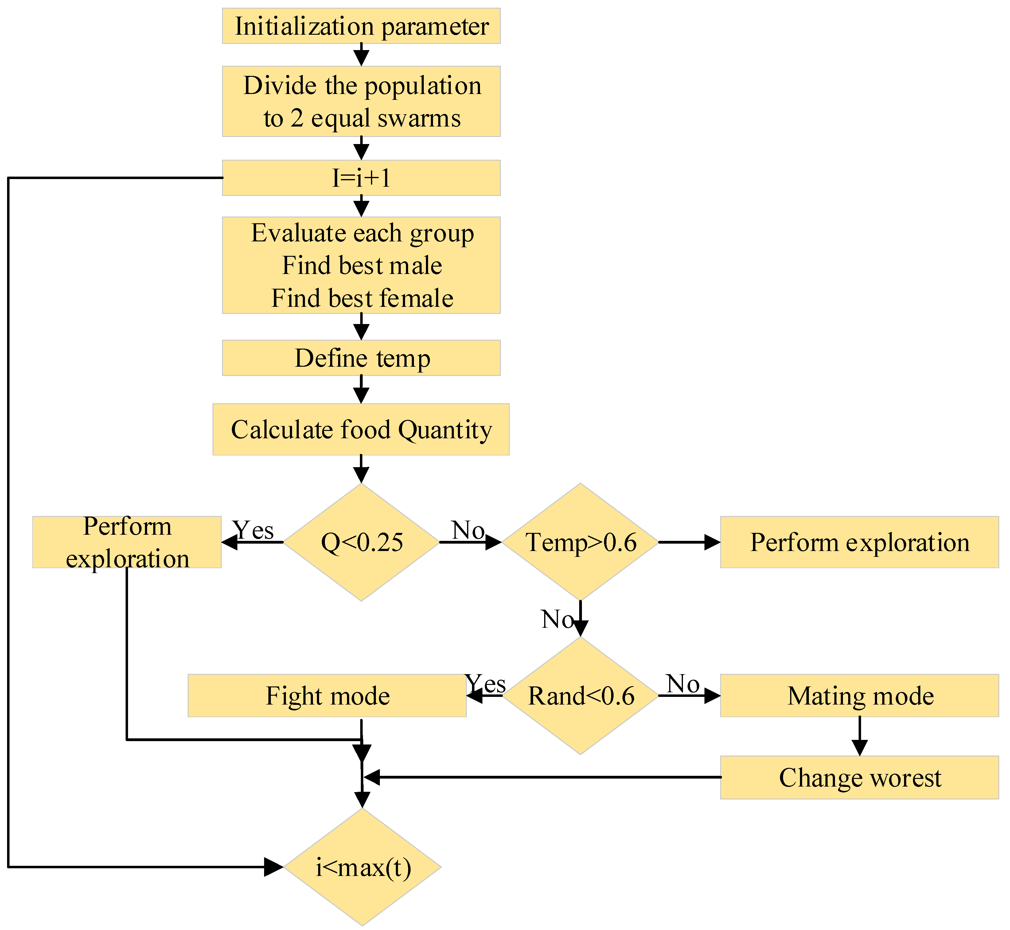
3.1.3. SO
3.1.4. Weight Value Calculation Based on PCA
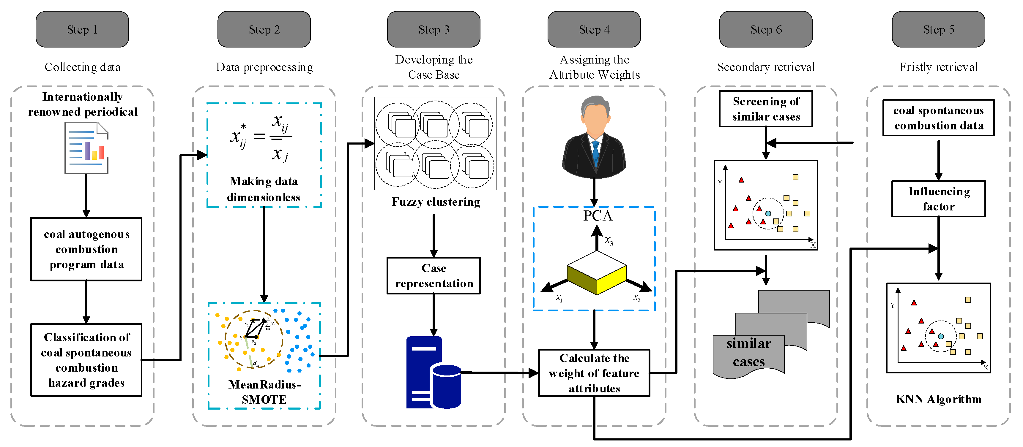
3.2. PCA-FC-CBR
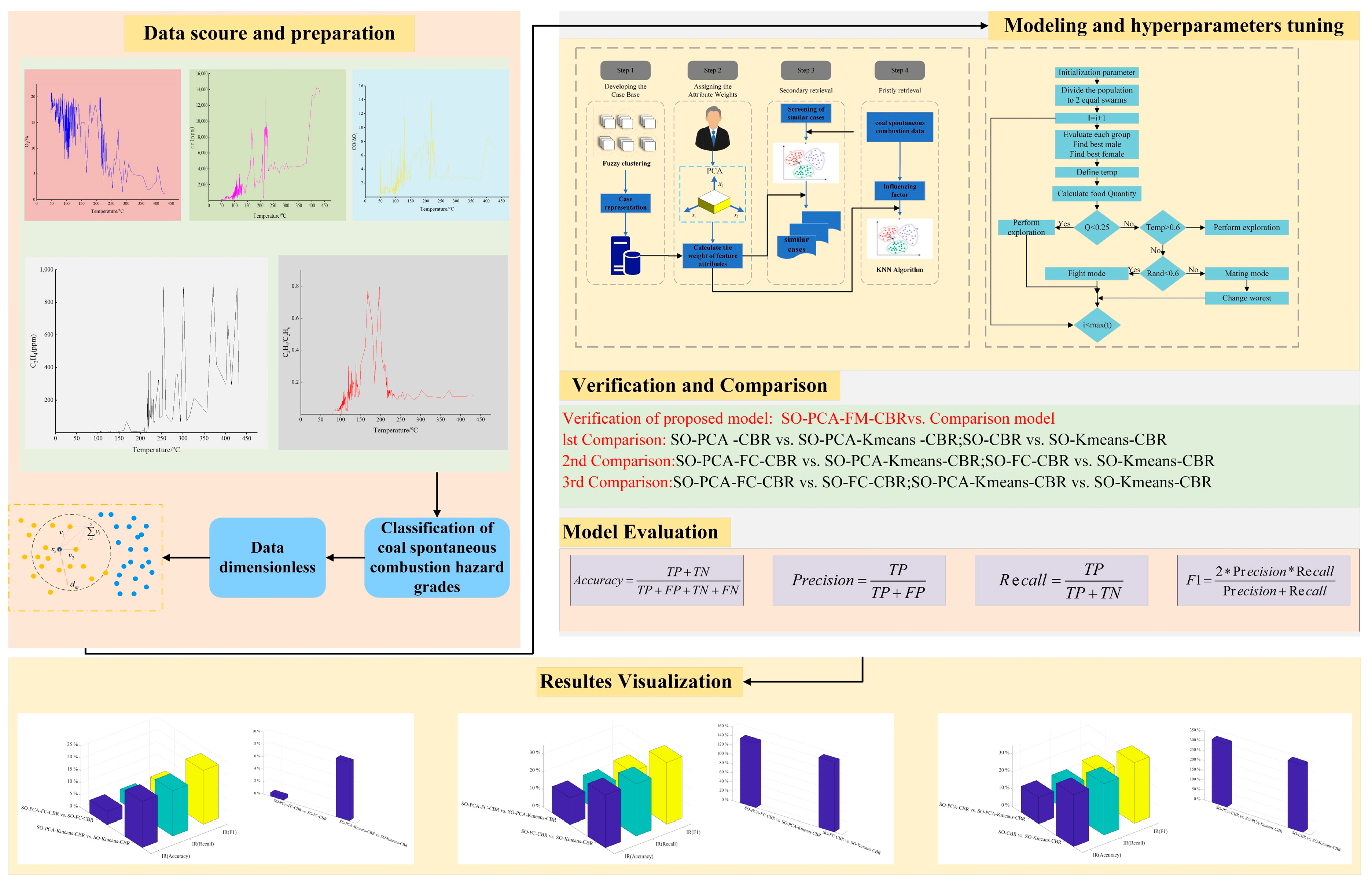
3.3. Modeling Building and Hyperparameter Tuning
3.3.1. Modeling Building
3.3.2. Hyperparameter Tuning
4. Experiments
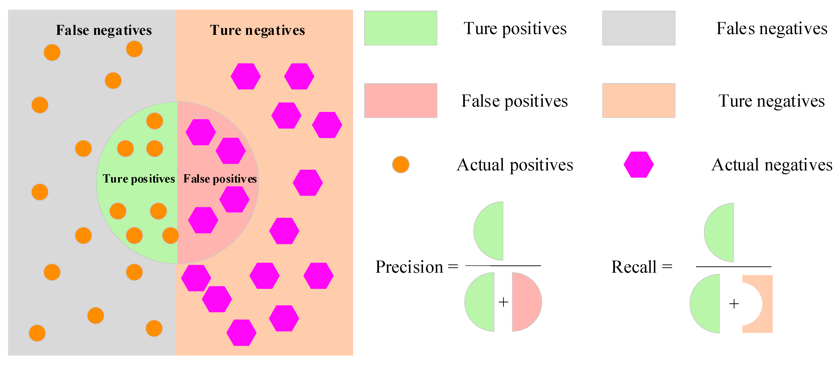
4.1. Dataset Division and Evaluation Indicators
4.2. Experiments and Comparison
5. Results and Discussions
5.1. Verification of Data Preprocessing Effect
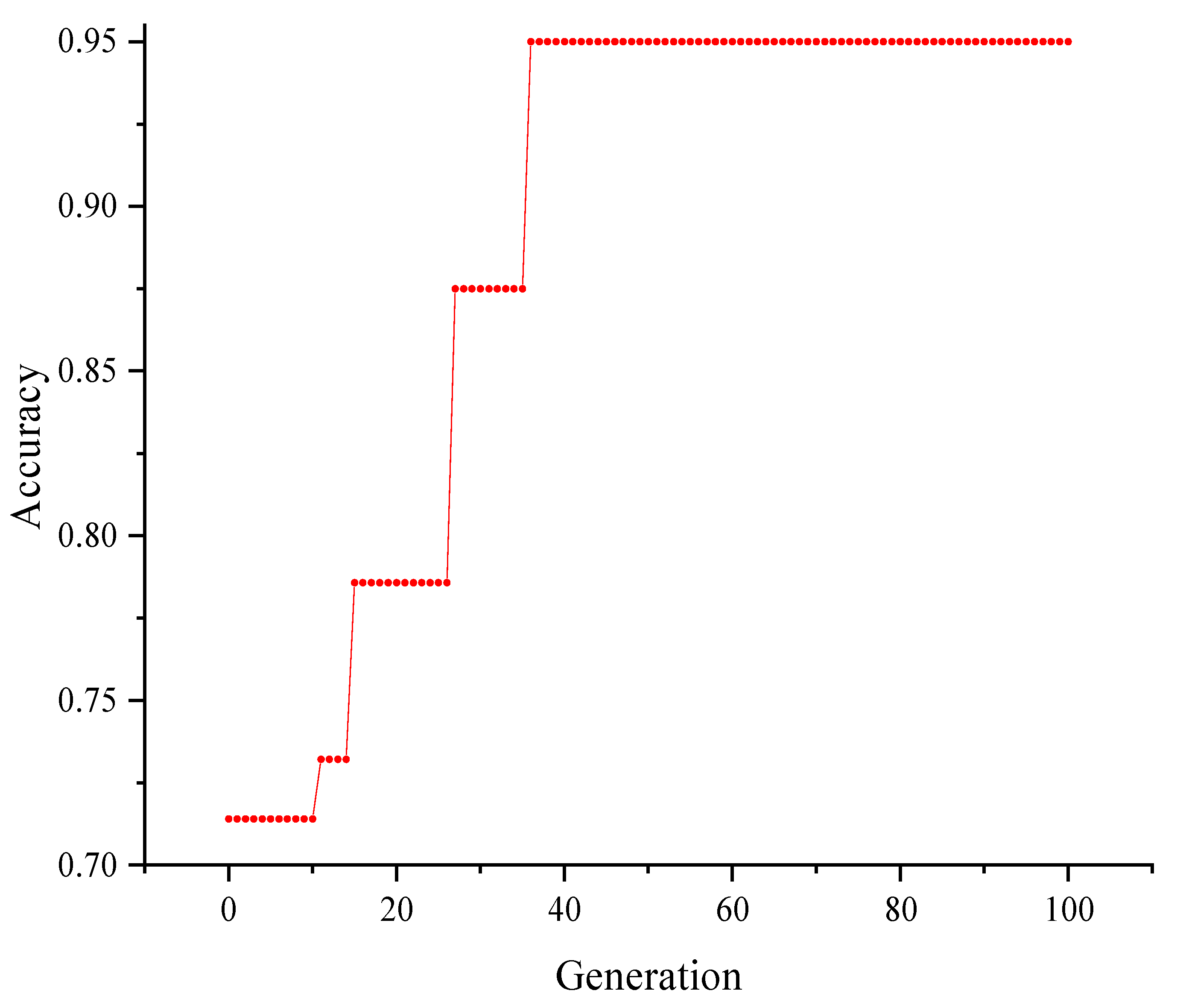
5.2. Parameter Tuning
5.3. Model Comparison Analysis
5.3.1. Comparison between SO–PCA–Clustering–CBR and Other Models
5.3.2. Comparison of Subgroups
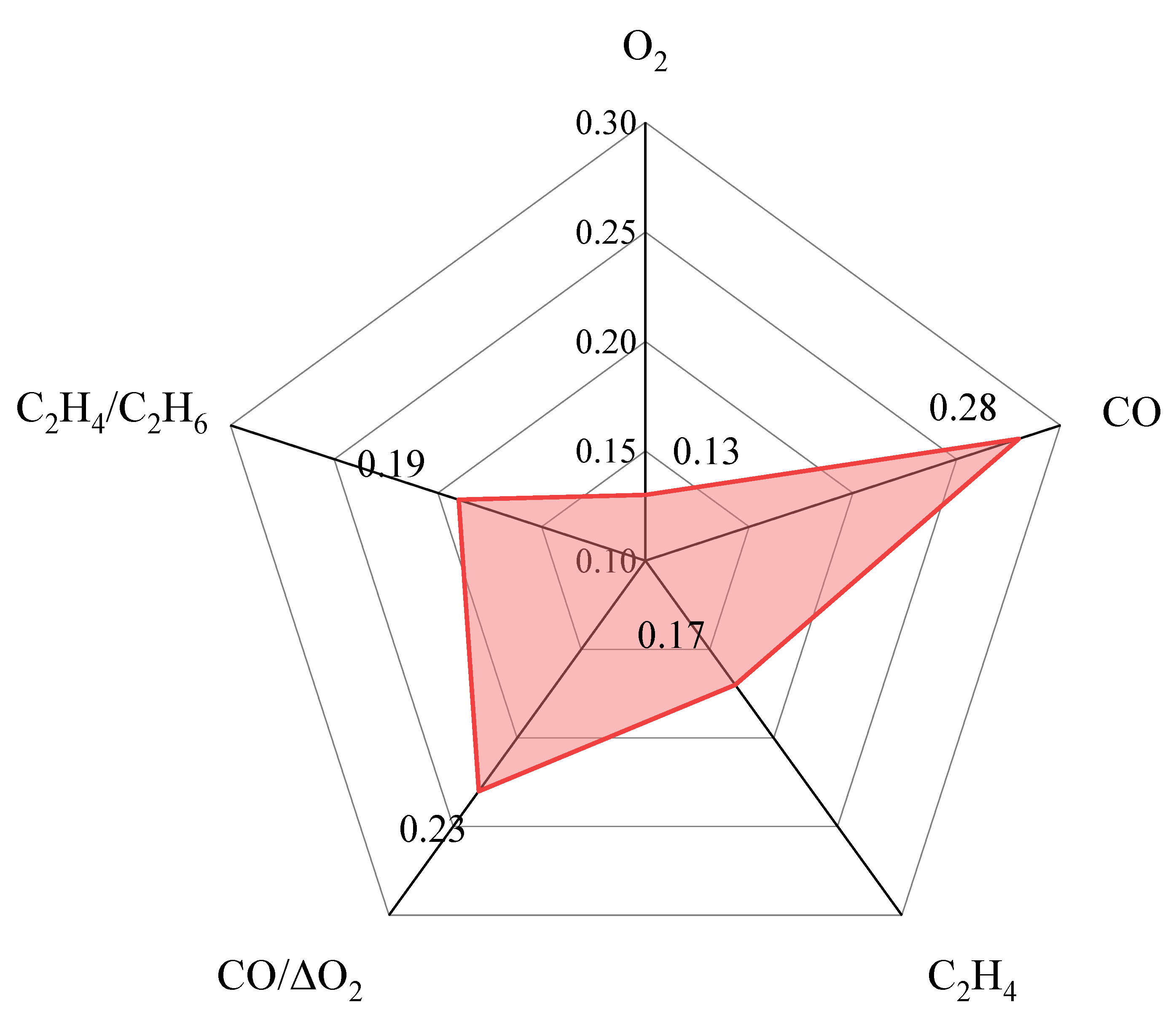
5.4. Variable Importance
6. Conclusions
- (1)
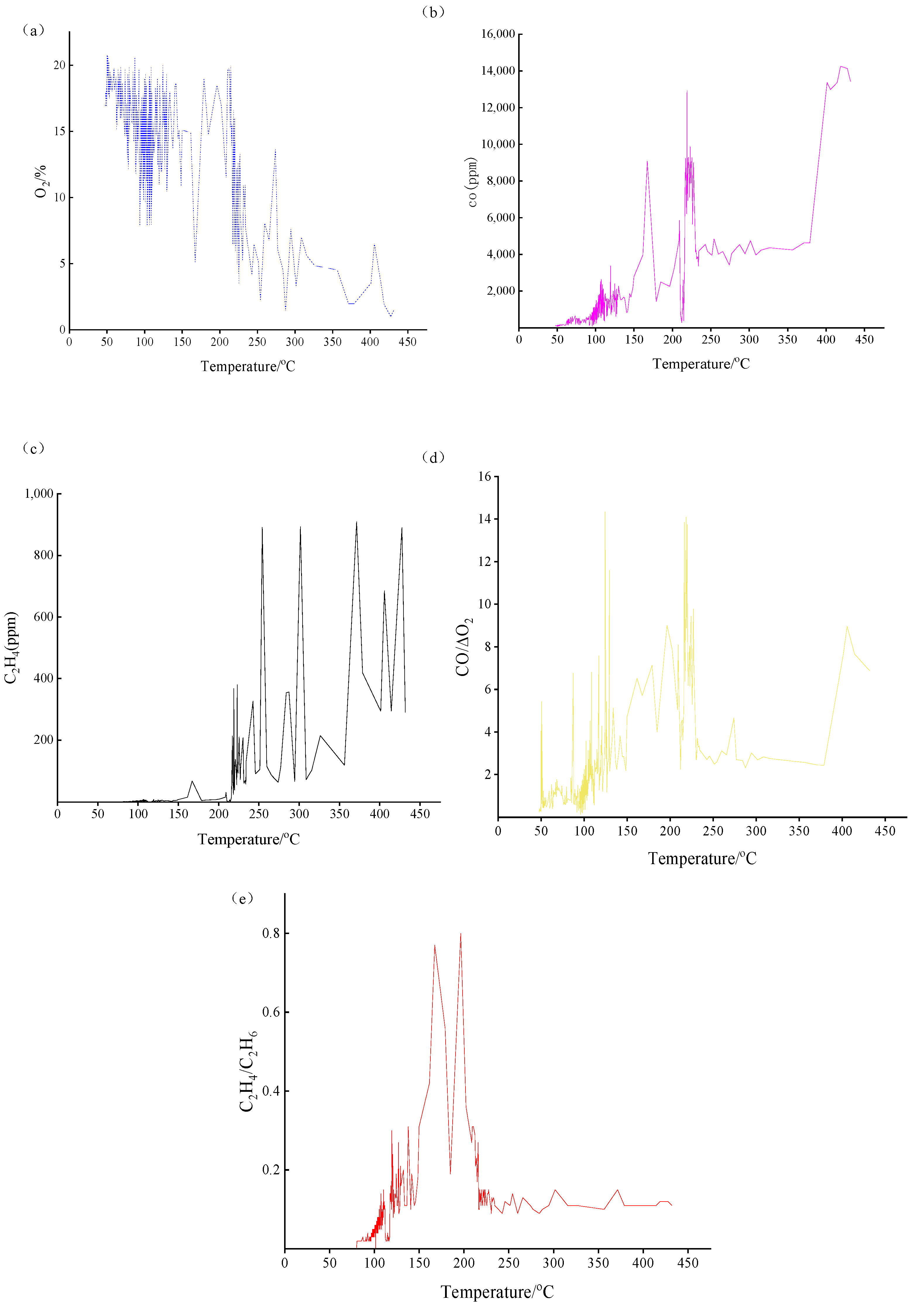
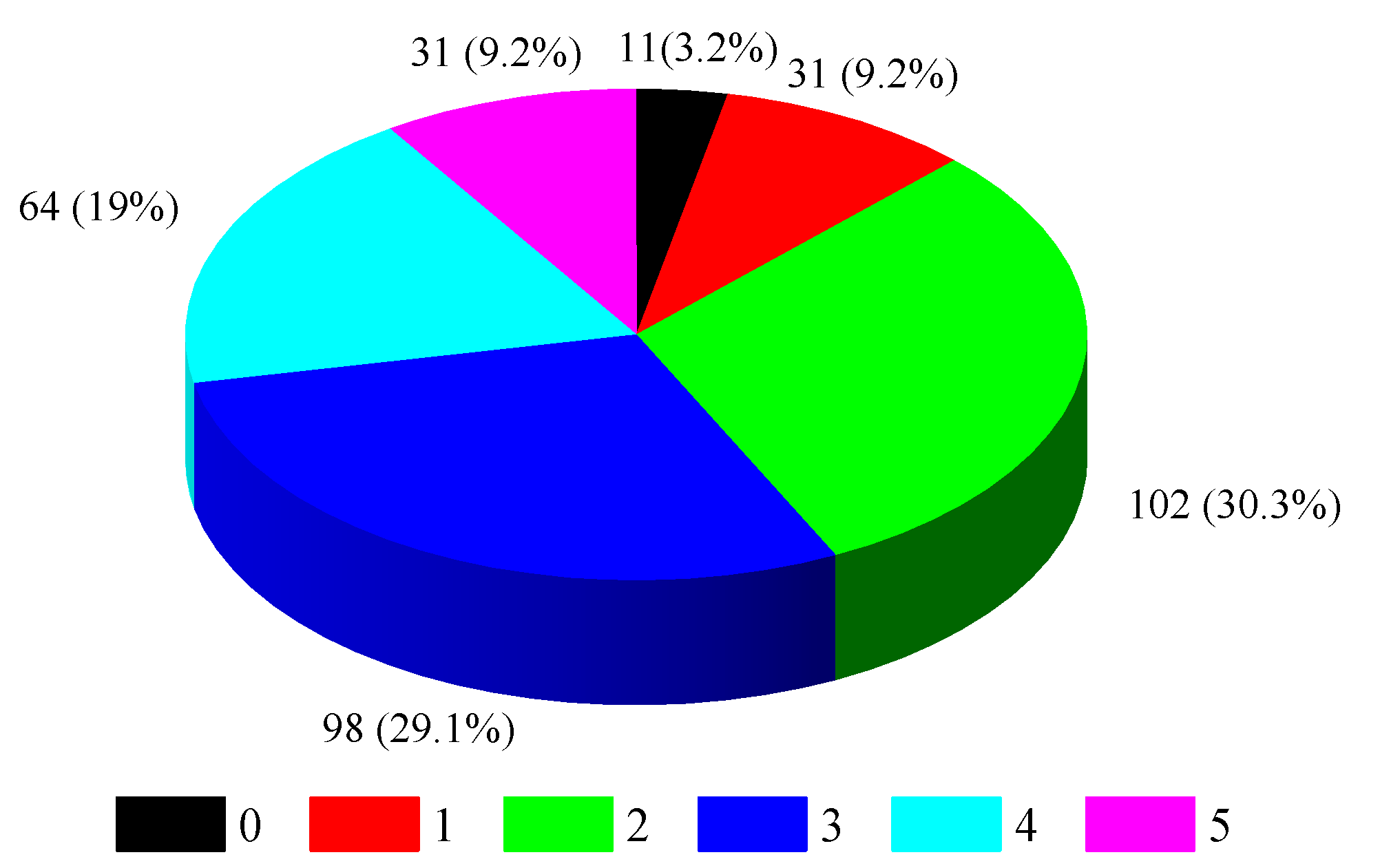
- By analyzing the change rule of the experimental data of heating up coal in the spontaneous combustion procedure, six characteristic temperatures and their thresholds were determined, and the hazard classes of coal were classified into six classes: green (0), blue (1), purple (2), yellow (3), orange (4), and red (5).
- (2)
- MeanRadius-SMOTE can be adopted to address the imbalance of the dataset. By comparing the predictive ability of four prediction models on different datasets, it was found that the proposed method performs the best when compared to the SMOTE and Kmeans–SMOTE methods.
- (3)
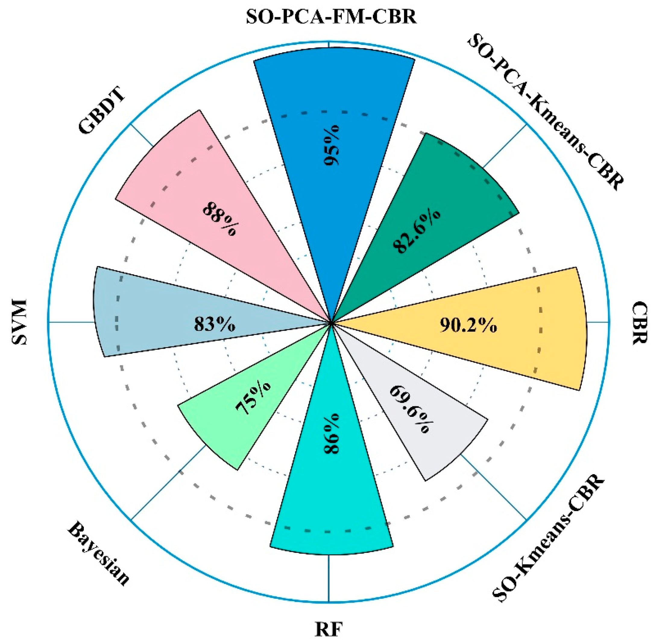
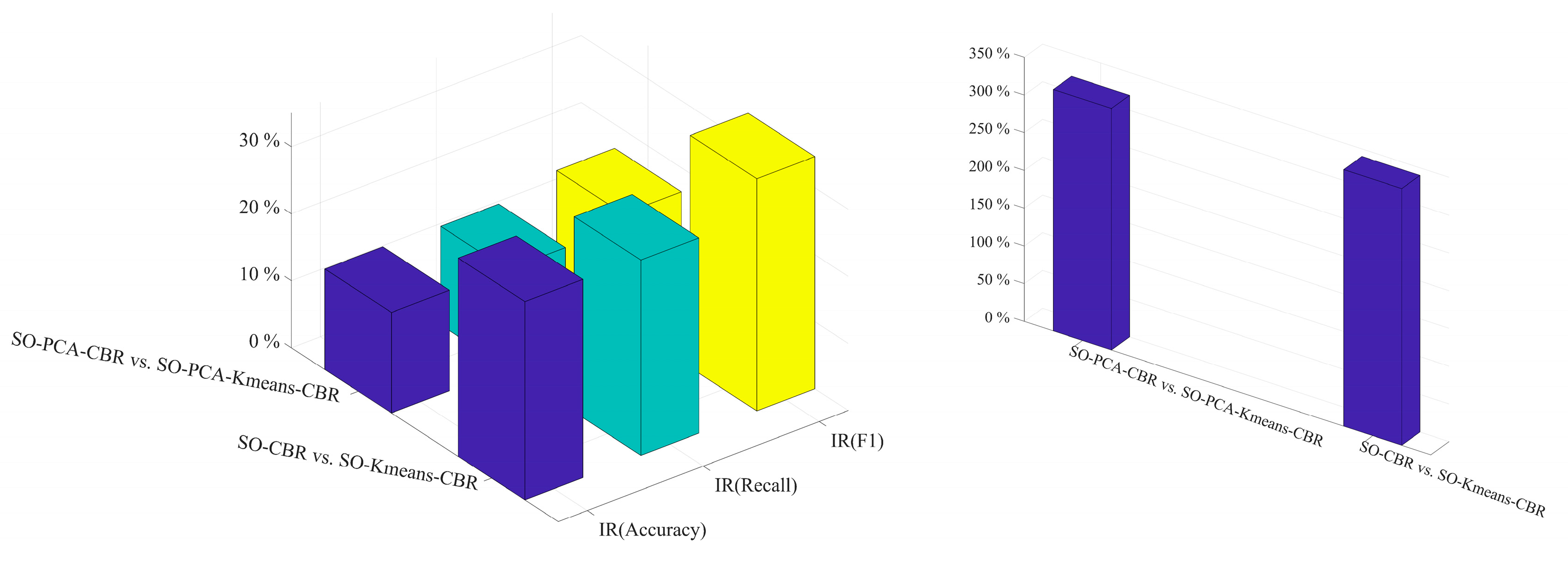
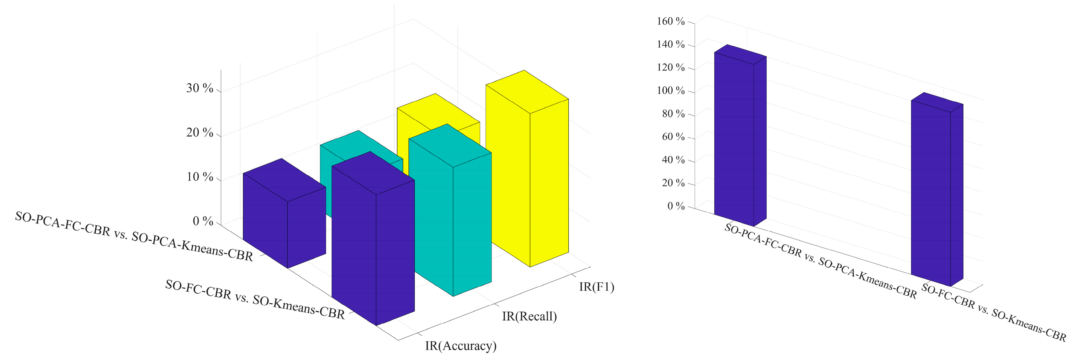
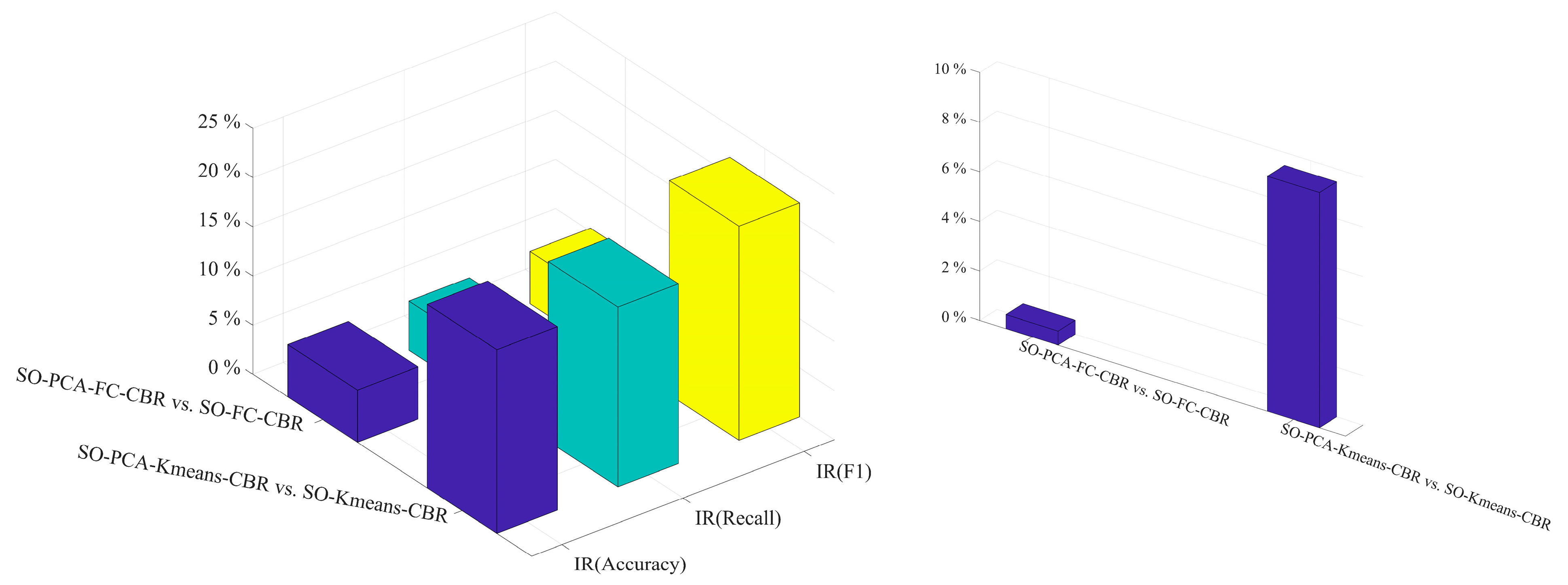
- Three sets of comparative experiments were conducted in this research to compare the performance of different machine learning models in predicting coal spontaneous combustion hazard grades. The experimental results indicate that (1) the traditional PCA–Clustering–CBR model reduces the computational cost but also causes boundary information loss, resulting in lower prediction accuracy of machine learning models; (2) compared with the traditional PCA–Clustering–CBR, fuzzy clustering avoids the loss of boundary information and improves the computational efficiency of the model without affecting the prediction accuracy; and (3) PCA can improve the prediction accuracy of machine learning models by calculating characteristic attribute weights based on the cumulative contribution rate.
- (4)
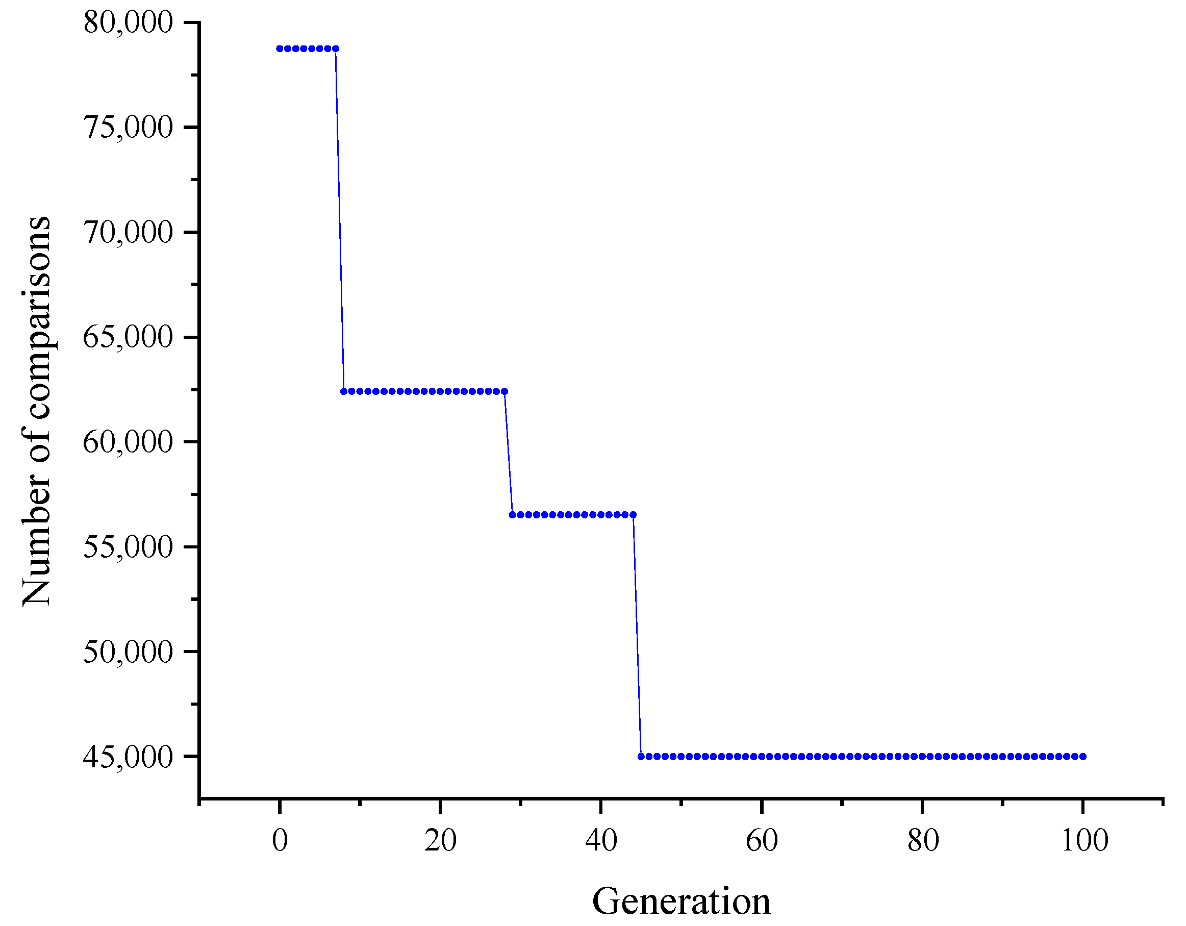
- Aiming at the multi-objective optimization problem of the PCA-FM-CBR model, this manuscript adopted the SO algorithm to optimize , and of the PCA-FM-CBR model step by step. The optimization shows that the model demonstrates optimal performance when the values of , and are 0.71, 0.39, and 2, respectively. The calculation cost is reduced to the greatest extent.
- (5)
- RBD-FAST was used to conduct sensitivity analysis for input variables, and the results demonstrated that CO is the most important input variable with a relative importance score of 0.28. Therefore, attention should be paid to CO in practical underground engineering.
Author Contributions
Funding
Institutional Review Board Statement
Informed Consent Statement
Data Availability Statement
Conflicts of Interest
References
- Wang, Y.M.; Liu, R.J.; Chen, X.Y.; Zou, X.Y.; Li, D.R.; Wang, S.S. Experimental Study on the Microstructural Characterization of Retardation Capacity of Microbial Inhibitors to Spontaneous Lignite Combustion. Fire 2023, 6, 20. [Google Scholar] [CrossRef]
- Wei, D.Y.; Du, C.F.; Lei, B.; Lin, Y.F. Prediction and prevention of spontaneous combustion of coal from goafs in workface: A case study. Case Stud. Therm. Eng. 2020, 21, 9. [Google Scholar] [CrossRef]
- Kursunoglu, N.; Gogebakan, M. Prediction of spontaneous coal combustion tendency using multinomial logistic regression. Int. J. Occup. Saf. Ergon. 2022, 28, 2000–2009. [Google Scholar] [CrossRef]
- Guo, J.; Yan, H.; Liu, Y.; Li, S.S. Preventing spontaneous combustion of coal from damaging ecological environment based on thermogravimetric analysis. Appl. Ecol. Environ. Res. 2019, 17, 9051–9064. [Google Scholar] [CrossRef]
- Lu, X.X.; Wang, M.Y.; Xue, X.; Xing, Y.; Shi, G.Y.; Shen, C.; Yang, Y.C.; Li, Y.B. An novel experimental study on the thermorunaway behavior and kinetic characteristics of oxidation coal in a low temperature reoxidation process. Fuel 2022, 310, 12. [Google Scholar] [CrossRef]
- Kong, B.; Li, Z.H.; Yang, Y.L.; Liu, Z.; Yan, D.C. A review on the mechanism, risk evaluation, and prevention of coal spontaneous combustion in China. Environ. Sci. Pollut. Res. 2017, 24, 23453–23470. [Google Scholar] [CrossRef]
- Wang, C.P.; Du, Y.X.; Deng, Y.; Zhang, Y.; Deng, J.; Zhao, X.Y.; Duan, X.D. Study on Spontaneous Combustion Characteristics and Early Warning of Coal in a Deep Mine. Fire 2023, 6, 18. [Google Scholar] [CrossRef]
- Wang, C.P.; Chen, L.J.; Bai, Z.J.; Deng, J.; Liu, L.; Xiao, Y. Study on the dynamic evolution law of spontaneous coal combustion in high-temperature regions. Fuel 2022, 314, 12. [Google Scholar] [CrossRef]
- Zhang, X.Q.; Zhou, F.Y.; Zou, J.X. Numerical Simulation of Gas Extraction in Coal Seam Strengthened by Static Blasting. Sustainability 2022, 14, 17. [Google Scholar] [CrossRef]
- Xu, G.; Li, K.G.; Li, M.L.; Qin, Q.C.; Yue, R. Rockburst Intensity Level Prediction Method Based on FA-SSA-PNN Model. Energies 2022, 15, 19. [Google Scholar] [CrossRef]
- Wang, J.F.; Liu, F.S.; Zhao, W.B.; Cai, H.L.; Zhao, J.; Liu, Y. Study on coal spontaneous combustion at low-medium temperature in the same coal seam with different buried depths and protolith temperatures. Int. J. Coal Prep. Util. 2022, 42, 3451–3463. [Google Scholar] [CrossRef]
- Liu, C.D.; Zhang, R.; Wang, Z.X.; Zhang, X.Q. Research on the fire extinguishing performance of new gel foam for preventing and controlling the spontaneous combustion of coal gangue. Environ. Sci. Pollut. Res. 2023, 30, 88548–88562. [Google Scholar] [CrossRef]
- Zhang, X.Q.; Pan, Y.Y. Preparation, Properties and Application of Gel Materials for Coal Gangue Control. Energies 2022, 15, 15. [Google Scholar] [CrossRef]
- Guo, Q.; Ren, W.X.; Lu, W. Risk evaluation of coal spontaneous combustion from the statistical characteristics of index gases. Thermochim. Acta 2022, 715, 10. [Google Scholar] [CrossRef]
- Li, S.; Xu, K.; Xue, G.Z.; Liu, J.; Xu, Z.Q. Prediction of coal spontaneous combustion temperature based on improved grey wolf optimizer algorithm and support vector regression. Fuel 2022, 324, 11. [Google Scholar] [CrossRef]
- Wang, F.S.; Xu, Y.Y.; Song, Z.Q.; Guo, L.W. Designing system predicting coal spontaneous combustion by means of method of gas analysis. In Proceedings of the 3rd International Symposium on Modern Mining and Safety Technology, Fuxin, China, 4–6 August 2008; pp. 326–328. [Google Scholar]
- Guo, Q.; Ren, W.X.; Lu, W. A Method for Predicting Coal Temperature Using CO with GA-SVR Model for Early Warning of the Spontaneous Combustion of Coal. Combust. Sci. Technol. 2022, 194, 523–538. [Google Scholar] [CrossRef]
- Shukla, R.; Khandelwal, M.; Kankar, P.K. Prediction and Assessment of Rock Burst Using Various Meta-heuristic Approaches. Min. Metall. Explor. 2021, 38, 1375–1381. [Google Scholar] [CrossRef]
- Zhang, L.D.; Song, Z.Y.; Wu, D.J.; Luo, Z.M.; Zhao, S.S.; Wang, Y.H.; Deng, J. Prediction of coal self-ignition tendency using machine learning. Fuel 2022, 325, 17. [Google Scholar] [CrossRef]
- Guo, J.; Chen, C.M.; Wen, H.; Cai, G.B.; Liu, Y. Prediction model of goaf coal temperature based on PSO-GRU deep neural network. Case Stud. Therm. Eng. 2024, 53, 13. [Google Scholar] [CrossRef]
- Wang, W.; Liang, R.; Qi, Y.; Cui, X.; Liu, J. Prediction model of spontaneous combustion risk of extraction borehole based on PSO-BPNN and its application. Sci. Rep. 2024, 14, 5. [Google Scholar] [CrossRef]
- Li, X.P.; Zhang, J.; Ren, X.P.; Liu, Y.Q.; Zhou, C.H.; Li, T.Y. Study on condition analysis and temperature prediction of coal spontaneous combustion based on improved genetic algorithm. AIP Adv. 2022, 12, 10. [Google Scholar] [CrossRef]
- Watson, I.; Marir, F. Case-based reasoning: A review. Knowl. Eng. Rev. 1994, 9, 327. [Google Scholar] [CrossRef]
- Deng, S.G.; Li, W.S. Spatial case revision in case-based reasoning for risk assessment of geological disasters. Geomat. Nat. Hazards Risk 2020, 11, 1052–1074. [Google Scholar] [CrossRef]
- Yang, S.K.; Bian, C.; Li, X.; Tan, L.; Tang, D.X. Optimized fault diagnosis based on FMEA-style CBR and BN for embedded software system. Int. J. Adv. Manuf. Technol. 2018, 94, 3441–3453. [Google Scholar] [CrossRef]
- Chen, M.Q.; Xia, J.Y.; Huang, R.Y.; Fang, W.G. Case-Based Reasoning System for Aeroengine Fault Diagnosis Enhanced with Attitudinal Choquet Integral. Appl. Sci. 2022, 12, 16. [Google Scholar] [CrossRef]
- Perez-Pons, M.E.; Parra-Dominguez, J.; Hernandez, G.; Bichindaritz, I.; Corchado, J.M. OCI-CBR: A hybrid model for decision support in preference-aware investment scenarios. Expert Syst. Appl. 2023, 211, 10. [Google Scholar] [CrossRef]
- Guerrero, J.I.; Miró-Amarante, G.; Martín, A. Decision support system in health care building design based on case-based reasoning and reinforcement learning. Expert Syst. Appl. 2022, 187, 7. [Google Scholar] [CrossRef]
- Zhao, Z.; Chen, J.H.; Yao, J.M.; Xu, K.H.; Liao, Y.Y.; Xie, H.W.; Gan, X.X. An improved spatial case-based reasoning considering multiple spatial drivers of geographic events and its application in landslide susceptibility mapping. Catena 2023, 223, 13. [Google Scholar] [CrossRef]
- Dorodnykh, N.; Nikolaychuk, O.; Pestova, J.; Yurin, A. Forest Fire Risk Forecasting with the Aid of Case-Based Reasoning. Appl. Sci. 2022, 12, 24. [Google Scholar] [CrossRef]
- Khan, M.J.; Hayat, H.; Awan, I. Hybrid case-base maintenance approach for modeling large scale case-based reasoning systems. Hum.-Centric Comput. Inf. Sci. 2019, 9, 25. [Google Scholar] [CrossRef]
- Liang, D.C.; Fu, Y.Y.; Xu, Z.S. Time-Varying Intuitionistic Fuzzy Integral for Emergency Materials Demand Prediction With Case-Based Reasoning. IEEE Trans. Fuzzy Syst. 2022, 30, 3617–3632. [Google Scholar] [CrossRef]
- Zhang, H.; Yang, J. A Case Retrieval Strategy for Traffic Congestion Based on Cluster Analysis. Math. Probl. Eng. 2022, 2022, 8. [Google Scholar] [CrossRef]
- Kuo, R.J.; Cha, C.L.; Chou, S.H. Developing a diagnostic system through the integration of ant colony optimization systems and case-based reasoning. Int. J. Adv. Manuf. Technol. 2006, 30, 750–760. [Google Scholar] [CrossRef]
- Lin, M.C.; He, D.B.; Sun, S.X. Multivariable Case Adaptation Method of Case-Based Reasoning Based on Multi-Case Clusters and Multi-Output Support Vector Machine for Equipment Maintenance Cost Prediction. IEEE Access 2021, 9, 151960–151971. [Google Scholar] [CrossRef]
- Khan, M.J.; Khan, C. Performance evaluation of fuzzy clustered case-based reasoning. J. Exp. Theor. Artif. Intell. 2021, 33, 313–330. [Google Scholar] [CrossRef]
- Wang, C.; Hu, P.; Sun, Y.; Yang, C. Study on CO source identification and spontaneous combustion warning concentration in the return corner of working face in shallow buried coal seam. Environ. Sci. Pollut. Res. 2024, 31, 15050–15064. [Google Scholar] [CrossRef]
- Li, L.; Ren, T.; Zhong, X.X.; Wang, J.T. Study of the Abnormal CO-Exceedance Phenomenon in the Tailgate Corner of a Low Metamorphic Coal Seam. Energies 2022, 15, 16. [Google Scholar] [CrossRef]
- Liang, Y.T.; Song, S.L.; Guo, B.L.; Gao, L.Y.; Liu, J.F.; Lu, W.; Wang, W.; Kong, B. Study on the Coupling Characteristics of Infrasound-Temperature-Gas in the Process of Coal Spontaneous Combustion and a New Early Warning Method. Combust. Sci. Technol. 2023. [Google Scholar] [CrossRef]
- Peng, J. Research on Prediction Model of Coal Spontaneous Combustion Temperature Based on Machine Learning. Master’s Thesis, Xi’an University of Science and Technology, Xi’an, China, 2020. [Google Scholar]
- Zhang, D.; Cen, X.X.; Wang, W.F.; Deng, J.; Wen, H.; Xiao, Y.; Shu, C.M. The graded warning method of coal spontaneous combustion in Tangjiahui Mine. Fuel 2021, 288, 7. [Google Scholar] [CrossRef]
- Xu, X.F.; Zhang, F.J. Evaluation and Optimization of Multi-Parameter Prediction Index for Coal Spontaneous Combustion Combined with Temperature Programmed Experiment. Fire 2023, 6, 15. [Google Scholar] [CrossRef]
- Lei, P. Study on Early warning technology of coal spontaneous combustion in goaf of Linhuan 9 Coal Seam. Master’s Thesis, Anhui University of Science and Technology, Anhui, China, 2022. [Google Scholar]
- Biao, F.J. Study on Stage Determination Theory and Classified Early Warning Method for Spontaneous Combustion of Coal. Ph.D. Thesis, Xi’an University of Science and Technology, Xi’an, China, 2019. [Google Scholar]
- Duan, F.; Zhang, S.; Yan, Y.; Cai, Z. An Oversampling Method of Unbalanced Data for Mechanical Fault Diagnosis Based on MeanRadius-SMOTE. Sensors 2022, 22, 5166. [Google Scholar] [CrossRef]
- Aamodt, A.; Plaza, E. Case-Based Reasoning: Foundational Issues, Methodological Variations, and System Approaches. AI Commun. 1994, 7, 39–59. [Google Scholar] [CrossRef]
- Wu, H.T.; Zhong, B.T.; Medjdoub, B.; Xing, X.J.; Jiao, L. An Ontological Metro Accident Case Retrieval Using CBR and NLP. Appl. Sci. 2020, 10, 24. [Google Scholar] [CrossRef]
- Askari, S. Fuzzy C-Means clustering algorithm for data with unequal cluster sizes and contaminated with noise and outliers: Review and development. Expert Syst. Appl. 2021, 165, 27. [Google Scholar] [CrossRef]
- Hashim, F.A.; Hussien, A.G. Snake Optimizer: A novel meta-heuristic optimization algorithm. Knowl.-Based Syst. 2022, 242, 34. [Google Scholar] [CrossRef]
- Zheng, W.M.; Pang, S.Y.; Liu, N.; Chai, Q.W.; Xu, L.D. A Compact Snake Optimization Algorithm in the Application of WKNN Fingerprint Localization. Sensors 2023, 23, 16. [Google Scholar] [CrossRef]
- Yan, X.; Tu, N.; Wu, S.; Zhu, Y. Dynamic Prediction of Coal and Gas Outburst Based on Clustering and Case-Based Reasoning. Chin. J. Sens. Actuators 2015, 28, 7. [Google Scholar]
- Trajdos, P.; Kurzynski, M. Weighting scheme for a pairwise multi-label classifier based on the fuzzy confusion matrix. Pattern Recognit. Lett. 2018, 103, 60–67. [Google Scholar] [CrossRef]
- Chawla, N.V.; Bowyer, K.W.; Hall, L.O.; Kegelmeyer, W.P. SMOTE: Synthetic Minority Over-sampling Technique. J. Artif. Intell. Res. 2002, 16, 321–357. [Google Scholar] [CrossRef]
- Fernandez, A.; Garcia, S.; Herrera, F.; Chawla, N.V. SMOTE for Learning from Imbalanced Data: Progress and Challenges, Marking the 15-year Anniversary. J. Artif. Intell. Res. 2018, 61, 863–905. [Google Scholar] [CrossRef]
- Douzas, G.; Bacao, F.; Last, F. Improving imbalanced learning through a heuristic oversampling method based on k-means and SMOTE. Inf. Sci. 2018, 465, 1–20. [Google Scholar] [CrossRef]
- Mara, T.A. Extension of the RBD-FAST method to the computation of global sensitivity indices. Reliab. Eng. Syst. Saf. 2009, 94, 1274–1281. [Google Scholar] [CrossRef]
- Gao, B.; Yang, Q.; Peng, Z.J.; Xie, W.H.; Jin, H.; Meng, S.H. A direct random sampling method for the Fourier amplitude sensitivity test of nonuniformly distributed uncertainty inputs and its application in C/C nozzles. Aerosp. Sci. Technol. 2020, 100, 8. [Google Scholar] [CrossRef]
- Xu, Q.; Yang, S.Q.; Cai, J.W.; Zhou, B.Z.; Xin, Y.A. Risk forecasting for spontaneous combustion of coals at different ranks due to free radicals and functional groups reaction. Process Saf. Environ. Protect. 2018, 118, 195–202. [Google Scholar] [CrossRef]
- Zhang, Y.T.; Shi, X.Q.; Li, Y.Q.; Liu, Y.R. Characteristics of carbon monoxide production and oxidation kinetics during the decaying process of coal spontaneous combustion. Can. J. Chem. Eng. 2018, 96, 1752–1761. [Google Scholar] [CrossRef]
- Yan, H.W.; Nie, B.S.; Liu, P.J.; Chen, Z.Y.; Yin, F.F.; Gong, J.; Lin, S.S.; Wang, X.T.; Kong, F.B.; Hou, Y.N. Experimental investigation and evaluation of influence of oxygen concentration on characteristic parameters of coal spontaneous combustion. Thermochim. Acta 2022, 717, 11. [Google Scholar] [CrossRef]
- Wu, K.; Yao, Q.; Chen, Y.; Zhao, P.T.; Xi, C.Z.; Zhao, Y.; Wang, Q. Dependence evaluation of factors influencing coal spontaneous ignition. Energy Sci. Eng. 2023, 11, 3738–3750. [Google Scholar] [CrossRef]
- Mohalik, N.K.; Lester, E.; Lowndes, I.S. Review of experimental methods to determine spontaneous combustion susceptibility of coal—Indian context. Int. J. Min. Reclam. Environ. 2017, 31, 301–332. [Google Scholar] [CrossRef]


| Coal Spontaneous Combustion Stage Name | Gas Characteristics |
|---|---|
| The first stage | Higher concentrations and no |
| The second stage | starts to appear |
| The third stage | starts to appear |
| The fourth stage | values show an increasing trend |
| The fifth stage | values show an increasing trend |
| The sixth stage | Maximum value |
| Coal Spontaneous Combustion Stage Name | Temperature °C | Coal Spontaneous Combustion Hazard Grades |
|---|---|---|
| The first stage | Green warning (0) | |
| The second stage | Blue warning (1) | |
| The third stage | Purple warning (2) | |
| The fourth stage | Yellow warning (3) | |
| The fifth stage | Orange warning (4) | |
| The sixth stage | Red warning (5) |
| Parameters | |||
|---|---|---|---|
| Ranges | [0, 1] | [0, 1] | [0, 10] |
| Model | Raw Data Base | Data Base Processed via SMOTE | Data Base Processed via Kmeans–SMOTE | Data Base Processed via MeanradiusSMOTE |
|---|---|---|---|---|
| GBDT | 0.59 | 0.71 | 0.8 | 0.88 |
| SVM | 0.52 | 0.64 | 0.79 | 0.826 |
| RF | 0.74 | 0.79 | 0.83 | 0.86 |
| Bayesian | 0.53 | 0.59 | 0.64 | 0.75 |
| Model | Metrics | 0 | 1 | 2 | 3 | 4 | 5 |
|---|---|---|---|---|---|---|---|
| SO-PCA-FC-CBR | F1 | 1.00 | 0.98 | 0.97 | 0.98 | 0.88 | 0.89 |
| Recall | 1.00 | 1.00 | 0.97 | 0.97 | 0.81 | 0.97 | |
| Accuracy | 1.00 | 0.97 | 0.97 | 1.00 | 0.96 | 0.83 | |
| SO-PCA-Kmeans-CBR | F1 | 0.97 | 0.87 | 0.77 | 0.77 | 0.61 | 0.91 |
| Recall | 1.00 | 0.94 | 0.67 | 0.90 | 0.47 | 1.00 | |
| Accuracy | 0.94 | 0.81 | 0.91 | 0.68 | 0.88 | 0.83 | |
| SO-Kmeans-CBR | F1 | 0.77 | 0.55 | 0.72 | 0.73 | 0.38 | 0.86 |
| Recall | 1.00 | 0.48 | 0.60 | 0.93 | 0.25 | 0.93 | |
| Accuracy | 0.63 | 0.65 | 0.90 | 0.60 | 0.80 | 0.80 | |
| CBR | F1 | 0.94 | 0.94 | 0.95 | 0.97 | 0.79 | 0.84 |
| Recall | 0.94 | 0.97 | 0.90 | 0.97 | 0.69 | 0.97 | |
| Accuracy | 0.94 | 0.91 | 1.00 | 0.97 | 0.92 | 0.74 | |
| SVM | F1 | 0.79 | 0.61 | 0.84 | 0.84 | 0.90 | 1.00 |
| Recall | 1.00 | 0.48 | 0.77 | 0.93 | 0.81 | 1.00 | |
| Accuracy | 0.65 | 0.83 | 0.92 | 0.76 | 1.00 | 1.00 | |
| RF | F1 | 0.85 | 0.79 | 0.95 | 0.97 | 0.80 | 0.86 |
| Recall | 1.00 | 0.68 | 0.90 | 1.00 | 0.66 | 1.00 | |
| Accuracy | 0.74 | 0.95 | 1.00 | 0.94 | 1.00 | 0.75 | |
| Bayesian | F1 | 0.82 | 0.71 | 0.77 | 0.76 | 0.47 | 0.87 |
| Recall | 0.87 | 0.74 | 0.67 | 0.93 | 0.31 | 1.00 | |
| Accuracy | 0.77 | 0.68 | 0.91 | 0.64 | 1.00 | 0.77 | |
| GBDT | F1 | 0.97 | 0.94 | 0.88 | 0.75 | 0.75 | 0.91 |
| Recall | 1.00 | 0.94 | 0.90 | 0.83 | 0.62 | 1.00 | |
| Accuracy | 0.94 | 0.94 | 0.87 | 0.69 | 0.95 | 0.84 |
| Comparison Groups | Description |
|---|---|
| 1st set of comparison | SO-PCA -CBR vs. SO-PCA-Kmeans-CBR SO-CBR vs. SO-Kmeans-CBR |
| 2nd set of comparison | SO-PCA-FC-CBR vs. SO-PCA-Kmeans-CBR SO-FC-CBR vs. SO-Kmeans-CBR |
| 3rd set of comparison | SO-PCA-FC-CBR vs. SO-FC-CBR SO-PCA-Kmeans-CBR vs. SO-Kmeans-CBR |
| SO-PCA-CBR vs. SO-PCA-Kmeans-CBR | SO-CBR vs. SO-Kmeans-CBR | |
|---|---|---|
| IR(Accuracy) | 15.01% | 29.59% |
| IR (Recall) | 14.73% | 29.14% |
| IR (F1) | 16.42% | 34.63% |
| IR (Number of comparisons) | 320.01% | 340% |
| SO-PCA-FC-CBR vs. SO-PCA-Kmeans-CBR | SO-FC-CBR vs. SO-Kmeans-CBR | |
|---|---|---|
| IR (Accuracy) | 15.01% | 29.59% |
| IR (Recall) | 14.73% | 29.14% |
| IR (F1) | 16.42% | 34.63% |
| IR (Number of comparisons) | 140.32% | 150.83% |
| SO-PCA-FC-CBR vs. SO-FC-CBR | SO-PCA-Kmeans-CBR vs. SO-Kmeans-CBR | |
|---|---|---|
| IR (Accuracy) | 5.32% | 18.68% |
| IR (Recall) | 5.01% | 18.29% |
| IR (F1) | 5.32% | 21.79% |
| IR (Number of comparisons) | 0.57% | 9.48% |
Disclaimer/Publisher’s Note: The statements, opinions and data contained in all publications are solely those of the individual author(s) and contributor(s) and not of MDPI and/or the editor(s). MDPI and/or the editor(s) disclaim responsibility for any injury to people or property resulting from any ideas, methods, instructions or products referred to in the content. |
© 2024 by the authors. Licensee MDPI, Basel, Switzerland. This article is an open access article distributed under the terms and conditions of the Creative Commons Attribution (CC BY) license (https://creativecommons.org/licenses/by/4.0/).
Share and Cite
Pei, Q.; Jia, Z.; Liu, J.; Wang, Y.; Wang, J.; Zhang, Y. Prediction of Coal Spontaneous Combustion Hazard Grades Based on Fuzzy Clustered Case-Based Reasoning. Fire 2024, 7, 107. https://doi.org/10.3390/fire7040107
Pei Q, Jia Z, Liu J, Wang Y, Wang J, Zhang Y. Prediction of Coal Spontaneous Combustion Hazard Grades Based on Fuzzy Clustered Case-Based Reasoning. Fire. 2024; 7(4):107. https://doi.org/10.3390/fire7040107
Chicago/Turabian StylePei, Qiuyan, Zhichao Jia, Jia Liu, Yi Wang, Junhui Wang, and Yanqi Zhang. 2024. "Prediction of Coal Spontaneous Combustion Hazard Grades Based on Fuzzy Clustered Case-Based Reasoning" Fire 7, no. 4: 107. https://doi.org/10.3390/fire7040107