Vegetation Cover Type Classification Using Cartographic Data for Prediction of Wildfire Behaviour

Abstract

Predicting the behaviour of wildfires can help save lives and reduce health, socioeconomic, and environmental impacts. Because wildfire behaviour is highly dependent on fuel type and distribution, their accurate estimation is paramount for accurate prediction of the fire propagation dynamics. This paper studies the effect of combining automated hyperparameter tuning with Bayesian optimisation and recursive feature elimination on the accuracy of three boosting (AdaB, XGB, CatB), two bagging (Random Forest, Extremely Randomised Trees), and three stacking ensemble models with respect to their ability to estimate the vegetation cover type from cartographic data. The models are trained on the University of California Irvine (UCI) cover type dataset using five-fold cross-validation. Feature importance scores are calculated and used in recursive feature elimination analysis to study the sensitivity of model accuracy to the different feature combinations. Our results indicate that the implemented fine-tuning procedure significantly affects the accuracy of all models investigated, with XGB achieving an overall accuracy of 97.1% slightly outperforming the others.

1. Introduction

Annually, wildfires burn an area of approximately 420 million hectares around the world [1], resulting in a broad range of health, socioeconomic, and environmental impacts. A fire regime is the pattern of fuel consumption, fire intensity (severity) and fire frequency characteristic of a given area over extended periods of time. A regime is characterised by fire seasonality, fuel type and distribution, topography, weather patterns, and impact on vegetation and soil [2,3]. Affected by climate change and increased land-use pressure, wildfires have progressively become more frequent and severe, with this trend predicted to continue [4,5]. Billions of dollars are spent every year to prevent or mitigate the negative impacts of wildfires [6].

There are three basic types of wildfires, namely ground fires, surface fires and crown fires. Ground fires burn organic material beneath the surface such as peat, roots and buried logs. They are smouldering fires typically ignited by a passing surface fire, though they can also be ignited directly. Surface fires burn fuels above the ground and below the canopy such as logs, leaves, grass and shrubs, whereas crown fires burn canopy fuels (typically with higher moisture and lower bulk density) [7]. Wildfires may be characterised by other features as well, such as the cause of ignition, physical properties, fire size, and type of fuel. Fuel properties (e.g., moisture, biomass, distribution) are required inputs into all fire behaviour models [6], whether in the form of a categorical vegetation type as in FARSITE [8], exact physical quantities as in FIRETEC [9] and WFDS [10], or a fuel gas bed as in FireProM-F [11,12] (after pyrolysis has occurred). Therefore, meaningful predictions of fire behaviour and propagation require precision in the fuel characterisation and distribution over the landscape [13,14]. Thus, fast and accurate mapping of land cover and vegetation type is crucial to support fire propagation prediction models, especially those aimed at real-time or faster simulations [12]. This information can support a range of fire management activities, including fire prevention, fire suppression, and evacuation [4,15,16,17]. Research to characterise vegetation is generally concerned with:

(i)

Capturing individual structural features such as height, diameter at breast height (DBH), branching structure, canopy volume, and single-tree biomass (e.g., [18]).

(ii)

Estimating vegetation properties over a landscape (metrics) such as canopy biomass, canopy fuel load (CFL), moisture content, canopy base height (CBH), and canopy bulk density (CBD) (e.g., [19,20,21,22]).

Some structural features are obtained directly, e.g., via traditional field measurements, while others are predicted using more easily measured variables. For example, single-tree biomass is traditionally estimated from tree measurements using allometric equations [23]. Although traditional methods can yield precise measurements and estimates of cover and biomass, they require intensive and challenging field work to collect data in a highly localised manner (not easily scalable) [24,25]. Conversely, single-tree biomass may be estimated from effective crown data obtained via laser scans [26], while three-dimensional point clouds generated by (terrestrial or aerial) laser scans are ideal for capturing the structural features of trees via tree segmentation [27].

Evidently, metrics such as the canopy biomass and CFL can be obtained from vegetation structural features (e.g., [28,29]). For instance, Crespo-Peremarch et al. [30] estimated canopy fuel variables such as above-ground biomass, CBD and CFL from LiDAR full-waveform data. Similarly, Hartley et al. [25] proposed using UAV laser scanning point clouds from which spatial and intensity metrics are extracted and used as predictor variables to estimate above-ground biomass and above-ground available fuel.

Because the type of fuel has a strong influence on fire behaviour [31], it is useful not only to characterise the fuel but also to classify the fuel type [25] (see [6,14,32]). Hartley et al. [25] used deep learning multi-class segmentation to classify fuel types from aerial imagery. Previous research indicates that the percentage cover of different fuel types can be a useful metric for estimating fuel load [25,33].

Modern research on fuel characterisation and fuel type classification centres around the use of laser scan point clouds and machine learning (ML) or Deep Learning (DL) methods for both, regression and classification tasks (e.g., [24]). Li et al. [34] investigated the effect of variable selection with three different ML algorithms, namely Linear Regression (LR), Random Forest (RF), and Extreme Gradient Boosting (XGB). Their results indicate that variable selection can significantly improve the accuracy of all models, especially for the XGB algorithm. In turn, Luo et al. [35] used feature selection algorithms along with RF, XGB, and Category Boosting (CatB) regression models to estimate the above-ground biomass in forests. Their results suggest that feature selection significantly affects model accuracy and that a combination of Recursive Feature Elimination (RFE) and CatB considerably outperforms other models. Recently, Carpenter et al. [27] proposed an unsupervised canopy-to-root pathing tree segmentation algorithm as a prerequisite for automatic forest mapping.

In an early study, Blackard and Dean [36] compared the accuracy of a Feed-Forward Neural Network (FFNN) model against the Gaussian Discriminant Analysis (GDA) algorithm in predicting forest cover types from cartographic variables. Using a large dataset, FFNN achieved an accuracy of $70.5\%$ compared to the $50.4\%$ accuracy achieved by GDA. Pierce et al. [37] used a RF model to map the forest canopy fuel in Lassen Volcanic National Park, California, by integrating ML and satellite imagery data. Patil and Sivagami [38] used a stacking of ensembles, namely RF, Extra Trees (XT) classifier, and Adaptive Boosting (AdaB) of XTs, integrated with a FFNN to improve the accuracy of forest cover classification. Their results show an overall accuracy of $87.5\%$. Macmichael and Si [39] achieved an overall accuracy of $97.01\%$, significantly outperforming all other models. They used a FFNN with five hidden layers combined with Principle Component Analysis (PCA) for feature selection, k-fold cross-validation, and model parameter optimisation. Samat et al. [40] proposed a GPU-accelerated CatB-forest method to increase the accuracy of hyperspectral image classification for land cover mapping. They concluded that even though the proposed method outperforms other models (including basic CatB), this comes at a high computational cost. In a recent study, Sjöqvist et al. [41] implemented three classifiers, namely RF, Naïve Bayes (NB), and Support Vector Machine (SVM), integrated with PCA for the classification of different cover types from cartographic variables using the University of California Irvine (UCI) cover type dataset. The combination of RF with PCA achieved an overall accuracy of $94.7\%$, with class-wise accuracy of $93.7\%$, $96.7\%$, $95\%$, $77.9\%$, $77\%$, $86\%$, and $94.5\%$ for Class 1 through Class 7, respectively. For the same dataset, Al Sameer et al. [42] achieved an overall accuracy of $93\%$ using XGB with PCA, whereas Kumar and Sinha [43] achieved an overall accuracy of $94.6\%$ using a RF classifier trained via ten-fold cross-validation tuned with a grid search algorithm. Comparing the results in [42] to those in [43], it appears that a RF model with automated hyperparameter tuning outperforms XGB with feature selection. This suggests that finding the optimal values of the hyperparameters may be more important than implementing a feature selection method.

Therefore, the present paper proposes the use of state-of-the-art ML algorithms and automated hyperparameter tuning based on Bayesian optimisation to improve the accuracy of vegetation cover type classification. Furthermore, recursive feature elimination is used to study the effect of feature selection on model accuracy. To the best of our knowledge, only a handful of studies have focused on using recent algorithms such as CatB, XGB, and the ensemble stacking technique for fuel type classification. In addition, feature selection and automated hyperparameter tuning have been proven to increase the accuracy of classification models in different studies (e.g., [44,45,46]). The remainder of this paper is organised as follows: the dataset, main ML methods used, and hyperparameter optimisation approach are presented in Section 2; the experimental results are presented in Section 3 and discussed in Section 4; and our conclusions are provided in Section 5.

2. Materials and Methods

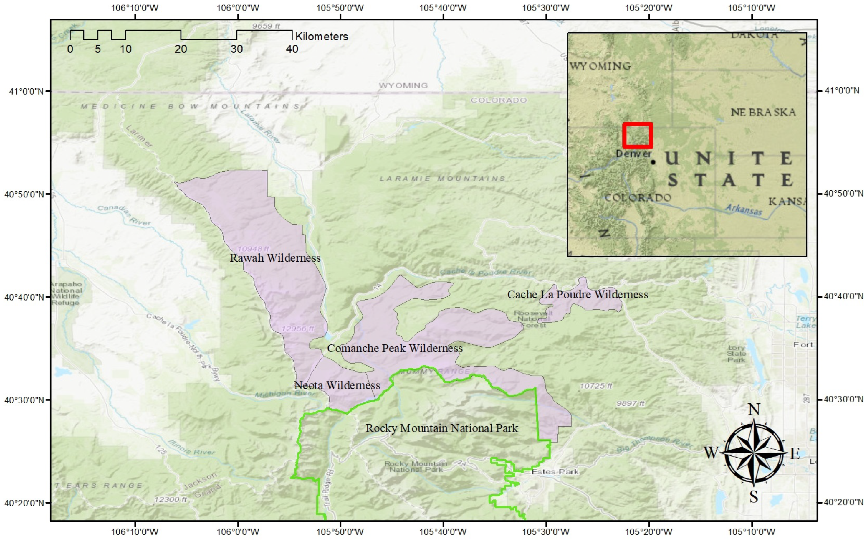
2.1. Dataset

This study uses the University of California Irvine (UCI) cover type dataset, which contains 581,012 datapoints, twelve features, and seven cover type categories. Observations are taken from four wilderness areas, namely (1) Neota (3904 ha), (2) Rawah (29,628 ha), (3) Comanche Peak (27,389 ha), and (4) Cache la Poudre (3817 ha) within the Roosevelt National Forest in Northern Colorado, 70 miles northwest of Denver [36] (see Figure 1).

The twelve features are: (1) elevation [m]; (2) aspect [degrees] (a.k.a. exposure or azimuth); (3) slope [degrees]; (4) horizontal distance to hydrology (HDH) [m]; (5) vertical distance to hydrology (VDH) [m]; (6) horizontal distance to roadway (HDR) [m]; (7) hillshade index at 9:00 am (HI9); (8) hillshade index at noon (HI12); (9) hillshade index at 3:00 pm (HI3); (10) wilderness area designation (four groups); (11) soil type designation (40 one-hot encoded soil types); and (12) horizontal distance to nearest wildfire ignition point (HDF) [m]. The seven forest cover type categories are: Spruce/Fir (C1), with 211,840 datapoints; Lodgepole Pine (C2), with 283,301 datapoints; Ponderosa Pine (C3), with 35,754 datapoints; Cottonwood/Willow (C4), with 2747 datapoints; Aspen (C5), with 9493 datapoints; Douglas Fir (C6), with 17,367 datapoints; and Krummholz (C7), with 20,510 datapoints. Generally, Neota has the highest mean elevation and is mainly covered with spruce/fir, while Rawah and Comanche Peak are mainly covered with lodgepole pine, spruce/fir, and aspen.

This dataset [36] was prepared using a combination of digital spatial data obtained from the US Geological Survey (USGS) and the US Forest Service (USFS). Thus, using digital elevation model (DEM) data with a resolution of 30 m, cartographic variables such as aspect, slope, and hillshade indices were extracted using the Geographic Information System (GIS). The distances from surface water resources were calculated by applying Euclidean distance analysis to the USGS hydrology and transport data, while soil type and wilderness areas were obtained from the USFS data. Hence a series of variables were obtained for each raster, comprising the input features into the classifier. Its output is the vegetation cover type.

In order to improve model performance, 5339 outliers based on the VDH were removed from the dataset, reducing the total number of datapoints to 575,576. This dataset was then split in two subsets, one for training the models ($70\%$) and the other for testing their accuracy ($30\%$). Pearson’s correlation coefficients (r) and associated p-values between different input features and the cover type are shown in Figure 2. Elevation, slope, wilderness area, and soil type are among the features showing higher correlation with the cover type. Because HI9 and HI3 were found to be highly correlated (Pearson’s $r=0.98$), the former was eliminated from the dataset and from Figure 2. The p-values show that the correlation coefficients (r) are statistically significant. The pairwise relationship of several of the most important features and their distributions are shown in Figure 3. It can be observed, for example, that elevation has a trimodal distribution, HDF and aspect have bimodal and right-skewed distributions, and HDH has a right-skewed distribution.

2.2. Base and Ensemble Learning Algorithms

2.2.1. Support Vector Machine

With applications in both classification and regression, SVM [48] is a form of supervised ML technique which relies in the use of spatial coordinates to assign training samples in order to maximise the distance between the categories. New samples are then projected into that same region and estimated to belong to one of many categories depending on which side of the gap they fall. The complexity of real-world problems frequently requires more precise assumptions than those provided by contemporary linear learning machines, which have certain processing limitations. Thus, it would be beneficial to examine more complex relationships such as polynomial and radial basis function kernels [49]. In this study, an SVM model with an RBF kernel is used as the first base model.

2.2.2. Decision Trees

Despite the difficulties of reaching a universality given their core structure, the class of supervised learning techniques known as Decision Trees (DTs) [50] represents an excellent example of a universal function approximator. Applications include regression and classification. A DT is made up of a number of branches connected by decision nodes, all of which end in leaf nodes. The decision node of the tree consists of a number of alternate leaf nodes that represent the output of the model, with each branch denoting a potential procedure. In classification and regression, this can be used as a label or a continuous value. The structure of the DT is largely composed of decision nodes. A basic goal when using this method is to minimise overfitting by using the shortest feasible tree. In an ensemble DT model (EDT), many trees are used either simultaneously (using bootstrap aggregation or bagging) or sequentially to produce a final model [6].

2.2.3. Random Forest

Random Forest (RF) is a mathematically solid ML method which aims to build more complex and robust models using bagging and random subspace as a base. Bagging is used to create a number of learner trees, which are then combined to obtain an overall prediction. Original training data are utilised to create bootstrap samples, which are then used to train the learning trees. A random selection of n instances from the initial training data (D), which consists of N instances, is used to construct each bootstrap sample (Db). Fresh instances may be used in place of the bootstrap samples. Db has a size of around two-thirds that of D, and does not have any duplicate instances [6]. The main idea behind RF entails building numerous “simple” Decision Trees (DTs) during training and using a majority voting method for classification. Among other advantages, this voting method corrects for the unfavourable tendency of DTs to overfit the training data [51].

Extremely Randomised Tree, or Extra Trees (XT) [52], is a tree-based method similar to RF that aims to increase accuracy by using the entire dataset rather than bootstrap samples to reduce bias, as well as to reduce the variance of the RF model by randomly selecting the optimal split points. Notably, XT executes faster than RF.

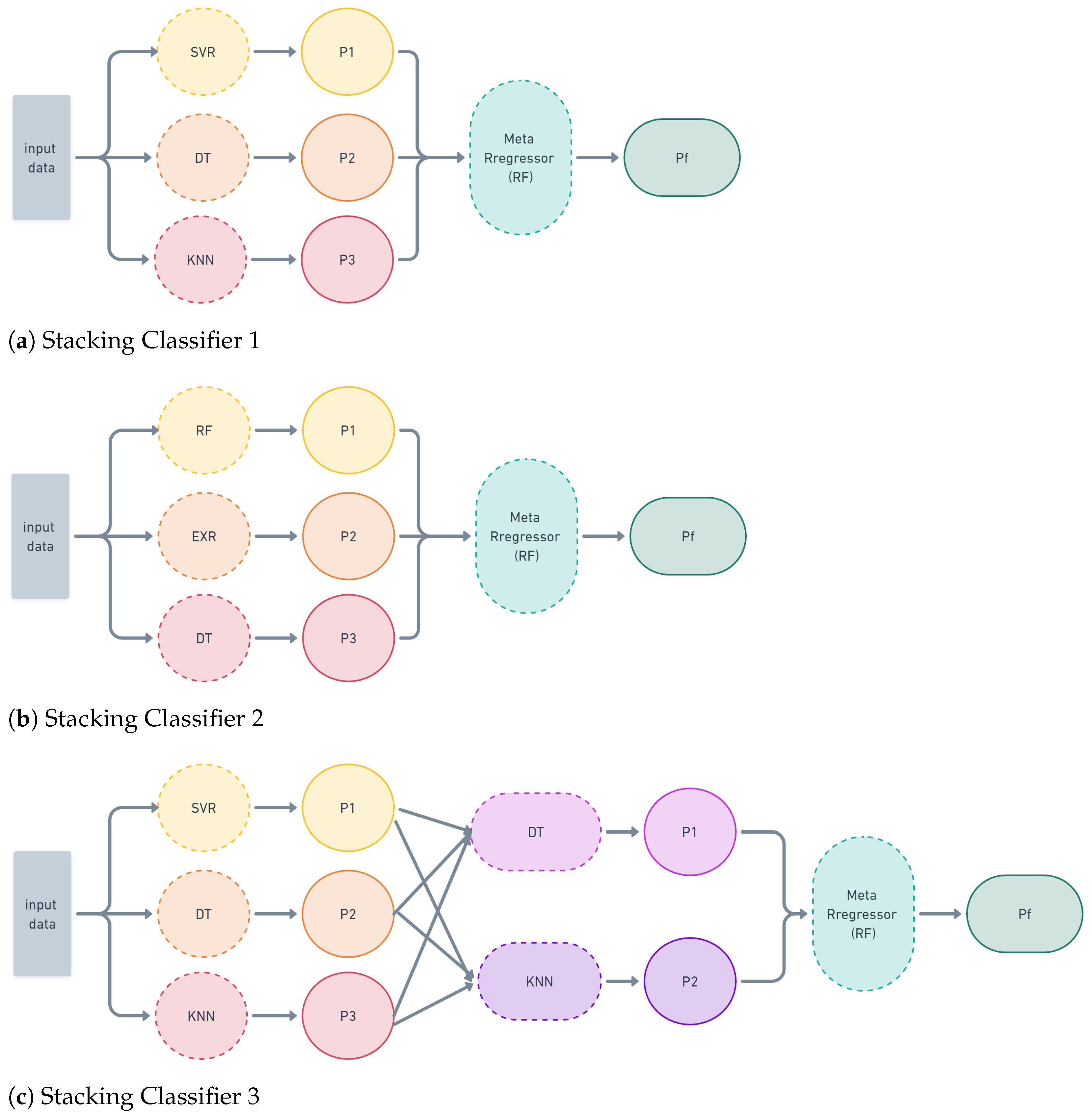
2.2.4. Stacked Models

The method of stacking regressions, initially introduced in [53], linearly combines several predictors to improve prediction accuracy. The approach primarily comprises two steps: $\left(i\right)$ specifying a list of base learners and training each one on the dataset, and ($ii$) using the predictions of the base learners as input to train the meta-learner, which then predicts new values.

The defined structures of the stacked models in this study are depicted in Figure 4. Three different Stacking Classifiers (SC1 to SC3) were constructed based on combinations of different optimised base and ensemble algorithms in order to produce more complex classifiers. For consistency, the meta-learner of all models is the optimised RF model.

2.2.5. Extreme Gradient Boosting

Gradient Boosting Decision Tree (GBDT) [54] is a supervised learning technique introduced by Jerome H. Friedman. Starting with a group of $(x_i,y_i)$ values, where $x_i$ stands for the input values and $y_i$ for the associated target values, it involves iteratively creating a set of functions $F^0$, $F^1$, … $F^t$, … $F^m$ which are then used to form the corresponding loss function $L(y_i,F^t)$ that estimates $y_i$. To enhance the accuracy of estimations, another function $F^{t+1}=F^t+h^{t+1}\left(x\right)$ is created to calculate $h^{t+1}$ as in Equation (1) [21,55]:

$$h^{t+1}=\underset{h\in H}{\arg \min }EL\left(y,F^t\right)$$

(1)

where H is the group of potential DTs being taken into account for the ensemble. Thus, the loss function can be defined as in Equation (2) [56]:

$$EL\left(y,F^{t+1}\right)=EL\left(y,F^t+h^{t+1}\right)$$

(2)

A variant of GBDT called Extreme Gradient Boosting (XGB) was developed by Chen and Guestrin [57]. In general, the XGB approach combines several base learners (DTs) to create an aggregated model that is more resilient.

Overfitting may result from incorrectly specifying DT parameters such as the depth or number of iterations. XGB penalises overfitted models by incorporating regularisation techniques. However, numerous hyperparameters need to be adjusted.

2.2.6. K-Nearest Neighbour

K-Nearest Neighbour (KNN or k-NN) is a supervised learning algorithm that can be used for both classification and regression tasks [58]. It aims to classify an unknown sample according to its distance to surrounding samples called neighbours. The defined context of distance is the Euclidian distance from the k-dimensional input vector $\overline{x}$ to its neighbour $\left(\overline{x_2}\right)$. In a regression context, the result is equal to the average of the target values over the desired k-nearest neighbours.

2.2.7. Adaptive Boosting

Adaptive Boosting (AdaB), formulated in [59], is a boosting ensemble that attempts to produce a strong learner by combining the outputs of weak base learners (though the method works for strong base learners as well), producing a stronger boosted classifier. AdaB attempts to learn from the mistakes of previous weak learners by increasing the weights assigned to incorrectly classified samples [60]. Higher weights are assigned to more accurate base learners.

2.2.8. Categorical Boosting

Categorical Boosting (CatB), proposed by Prokhorenkova et al. [61], is an enhanced variant of GBDT. It has several advantages over the basic GBDT model:

• It is generally more rigorous at handling categorical data, and uses one-hot encoding for categories with low cardinality.
• It utilises the Ordered Boosting technique, which means that it is able to use the same examples used for computation of Ordered Target Statistics to compute $h^{t+1}$ by assuming D to be the set of all available data for training the GBDT model, keeping in mind that the DT $h^{t+1}$ is the tree that minimises the loss function $\left(L\right)$.
• Its approach to building DTs relies heavily on Oblivious Decision Trees (ODTs). CatB creates a number of ODTs, which are full binary trees. Hence, there will be $2n$ nodes if there are n levels. The ODT’s non-leaf nodes divide according to the same standard. In order to increase confidence in the selection of the most productive feature combinations by CatB during training, the capabilities of GBDT are expanded to enable it to consider feature interactions. [56,61].

Since CatB is highly sensitive to its hyperparameters’ settings, their tuning is crucial.

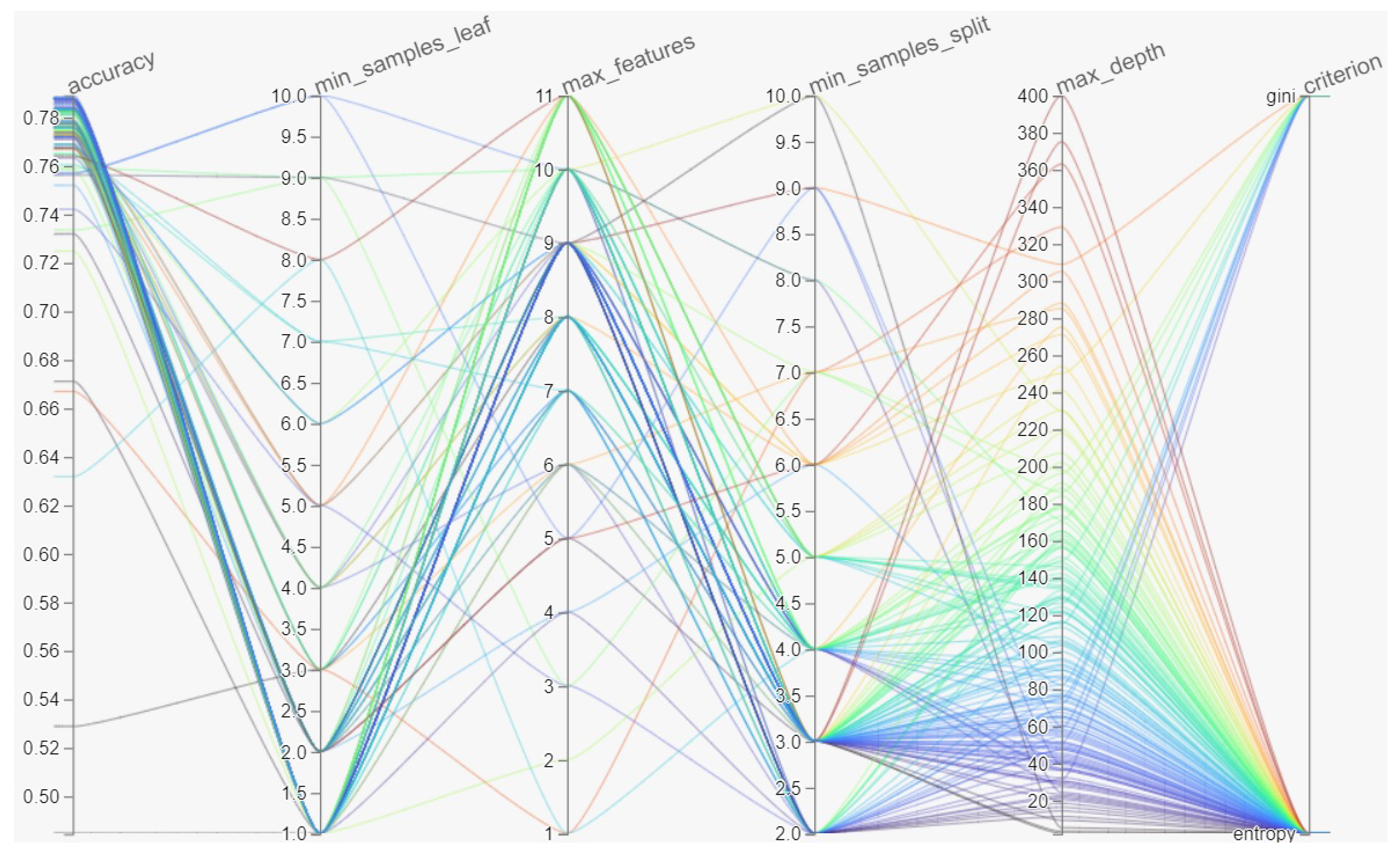
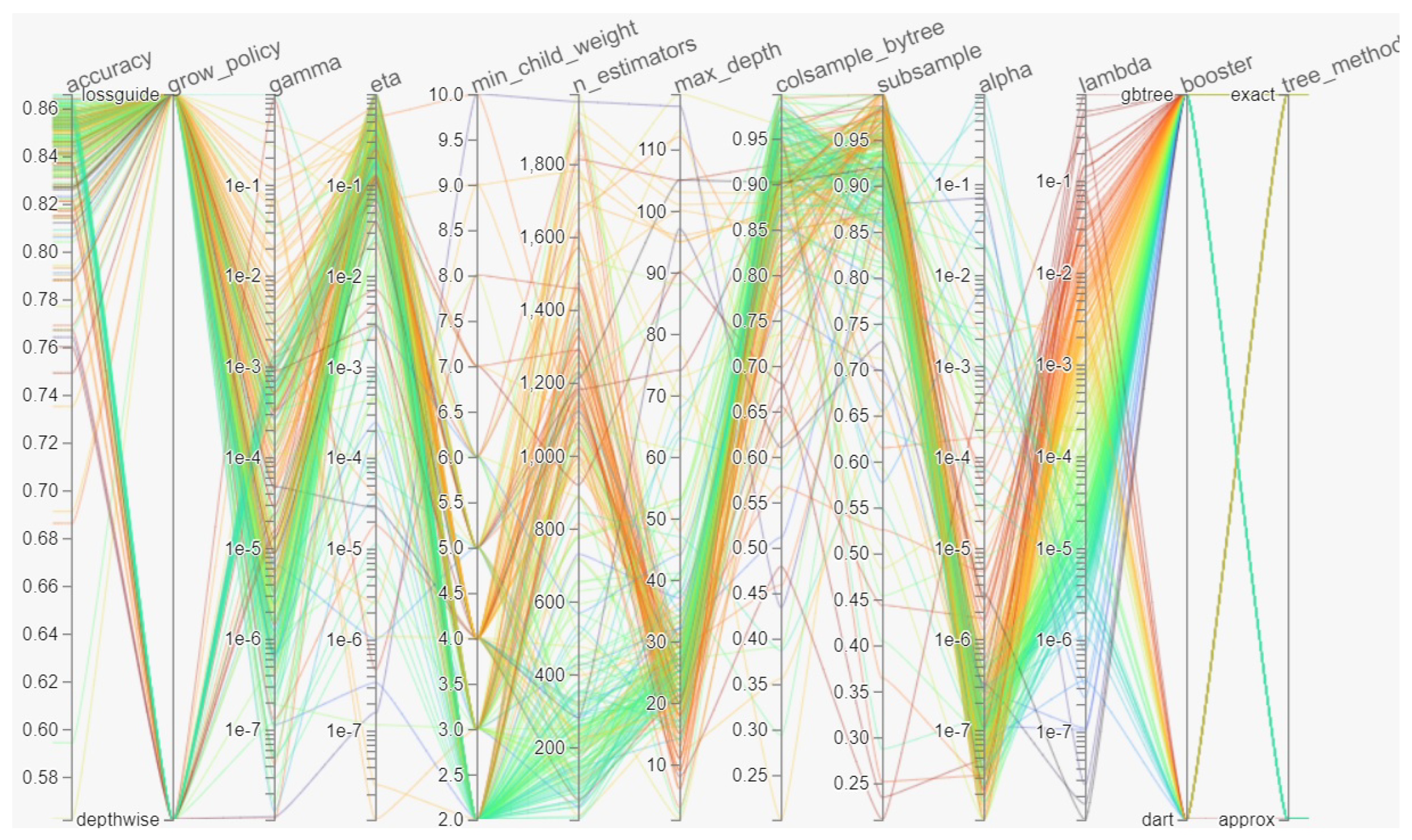
2.3. Hyperparameter Optimisation

The performance of a ML model can be greatly improved by using AutoML (short for Automated ML), which automates complicated tasks without the need for human understanding [62]. A crucial process is the optimal tuning of its hyperparameters.

Bayesian optimisation is a robust and potent technique for determining the extreme values of computationally difficult functions [63]. It can be used to optimise functions which are non-convex or those with derivatives that are challenging to calculate or evaluate [64]. Assuming that $\mathcal{F}:X\to \mathbb{R}$ is a well-behaved function defined on subset $X\subset {\mathbb{R}}^d$, the optimisation problem is formulated as shown in Equation (3).

$${\mathbf{x}}^{*}=\underset{\mathbf{x}\in X}{\arg \max }\mathcal{F}\left(\mathbf{x}\right)$$

(3)

Bayesian Optimisation assumes $\mathcal{F}\left(\mathbf{x}\right)$ to be unknown and treats it as stochastic, with a prior probability distribution that captures the beliefs about its structure. After collecting function evaluation data, the distribution is updated (the posterior distribution) and used to sample the next query point. Gaussian processes such as Kriging are typically used to define the probability distributions over $\mathcal{F}\left(\mathbf{x}\right)$.

Bayesian optimisation is frequently used for optimal hyperparameter tuning [65]. In this study, it is used to automatically tune all models’ hyperparameters separately using the Optuna library [66]. The dataset is relatively large and highly imbalanced, with 211,840 datapoints for the C1, 283,301 datapoints for the C2, and 2,747 datapoints for the C4 cover types. This results in an imbalance ratio of $N_{\max }/N_{\min }=77.1$. Therefore, we used random under-sampling to ensure a balanced dataset, with 2700 datapoints for each cover type extracted from the general dataset. Hyperparameter tuning was then performed on the smaller dataset using five-fold cross-validation for the model training corresponding to each candidate set of hyperparameters. Models were finally trained on the whole dataset with the obtained optimal set of hyperparameters, again using five-fold cross-validation.

Figure 5 and Figure 6 show the multi-dimensional space of the hyperparameters searched during fine-tuning of the DT and XGB models. For each iteration, the corresponding values of the hyperparameters are linked to the resulting accuracy. The model parameters obtained from the optimisation process for all models are presented in

Table 1. Hyperparameters for base learners and bagging ensembles.

SVR	DT	RF	XT
$Kernel=RBF$	$Splitter:best$	$Splitter:best$
$tolerance=0.483$	$Criterion:entropy$	$Criterion:entropy$	$Criterion:entropy$
$Regularization\left(C\right)=8.75$	$Minsamplesplit=3$	$Minsamplesplit=2$	$Minsamplesplit=2$
$gamma=0.4$	$Minsampleleaf=1$	$Minsampleleaf=1$	$Minsampleleaf=1$
$DecisionFunction:’\mathrm{ovo}’$	$Maxdepth=23$	$Maxdepth=25$	$Maxdepth=25$
		$N_{\mathrm{estimators}}=348$	$N_{\mathrm{estimators}}=348$

and

Table 2. Hyperparameters for boosting ensembles.

AdaB	XGB	CatB
$Bas{e}_{\mathrm{estimator}}=DT$	$objective=’\mathrm{multi}:\mathrm{softprob}’$	$iterations=$ 3500
$N_{\mathrm{estimators}}=180$	$N_{\mathrm{estimators}}=$ 1073	$loss\_functionMultiClassOneVsAll$
$Learningrate=1.2$	$eta=0.274$	$Learningrate=0.47$
$algorithm=’\mathrm{SAMME}’$	$maxdepth=25$	$depth=10$
	$subsample=0.5$	$subsample=0.8$
	$colsamplebytree=0.6$	$l2\_leaf\_reg=2.44$
	$treemethod=’\mathrm{exact}’$	$model\_size\_reg=2.62$
	$booster=’\mathrm{gbtree}’$	$bootstraptype:’\mathrm{Bernoulli}’$
	$minchildweight=2$	$boostingtype:’\mathrm{Plain}’$
	$growpolicy=’\mathrm{lossguide}’$
	$lambda=2.55\times {10}^{-5}$
	$alpha=3.95\times {10}^{-7}$

.

2.4. Model Development and Accuracy Assessment

The models in this paper made use of the Scikit-learn library [67], XGBoost library [68], and CatBoost [69] library. Four measures were used to evaluate the accuracy of the models: accuracy, precision, recall, and F1 score.

• Accuracy is defined as the ratio of correct predictions over the total number of instances evaluated, and is calculated as in Equation (4).

  $$acc=\frac{tp+tn}{tp+tn+fp+fn}$$

  (4)
• Precision is defined as positive patterns that are correctly predicted from the total predicted patterns in a positive class, and is calculated as in Equation (5).

  $$prec=\frac{tp}{tp+fp}$$

  (5)
• Recall is defined as the percentage of positive patterns that are correctly categorised, as in Equation (6).

  $$rec=\frac{tp}{tp+tn}$$

  (6)
• F1 score is the harmonic mean between recall and precision, and is calculated as in Equation (7) [70].

  $$F1=\frac{2·prec·rec}{prec+rec}$$

  (7)

3. Results

3.1. Model Feature Importance

Increasing model accuracy via feature selection is an important step when implementing ML algorithms, especially for high-dimensional data structures. A reliable approach to selecting the features which contribute the most and removing those which are detrimental is through feature importance analysis. The relative importance of features for the RF, XT, XGB, and CatB models is shown in Figure 7. The stacked models are not included here due to their hierarchical model fitting procedure.

It can be observed, for instance, that the slope of the terrain, HI12, and HI3 are among the least important features in the dataset.

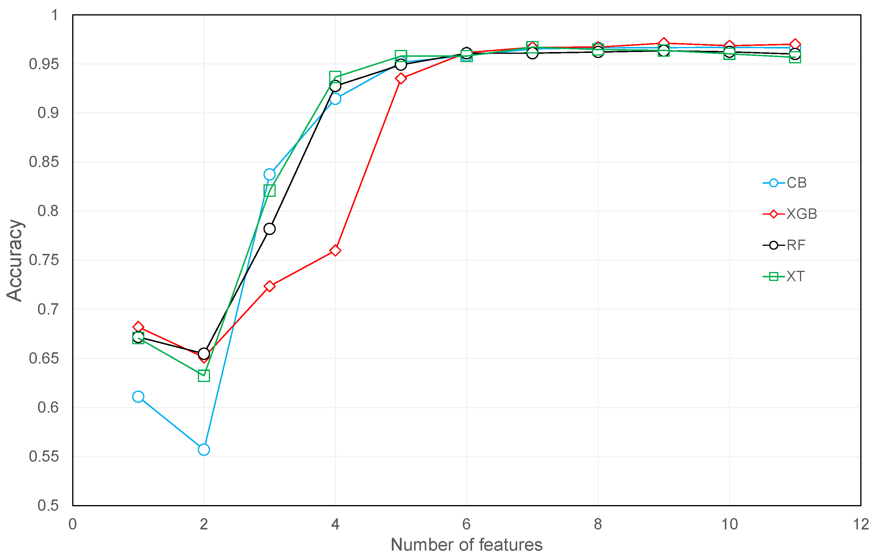
3.2. Recursive Feature Elimination

Recursive Feature elimination is a feature selection technique which eliminates the weakest feature(s) from a model in a sequential manner until it reaches an optimal or predefined number of features. The obtained accuracy of the RF, XT, XGB, and CatB models during recursive feature elimination analysis is presented in Figure 8 for an increasing number of features. The highest accuracy for CatB is obtained using ten features, excluding slope. For XGB and RF, the maximum accuracy is obtained using nine features, while XT achieves maximum accuracy using only seven features.

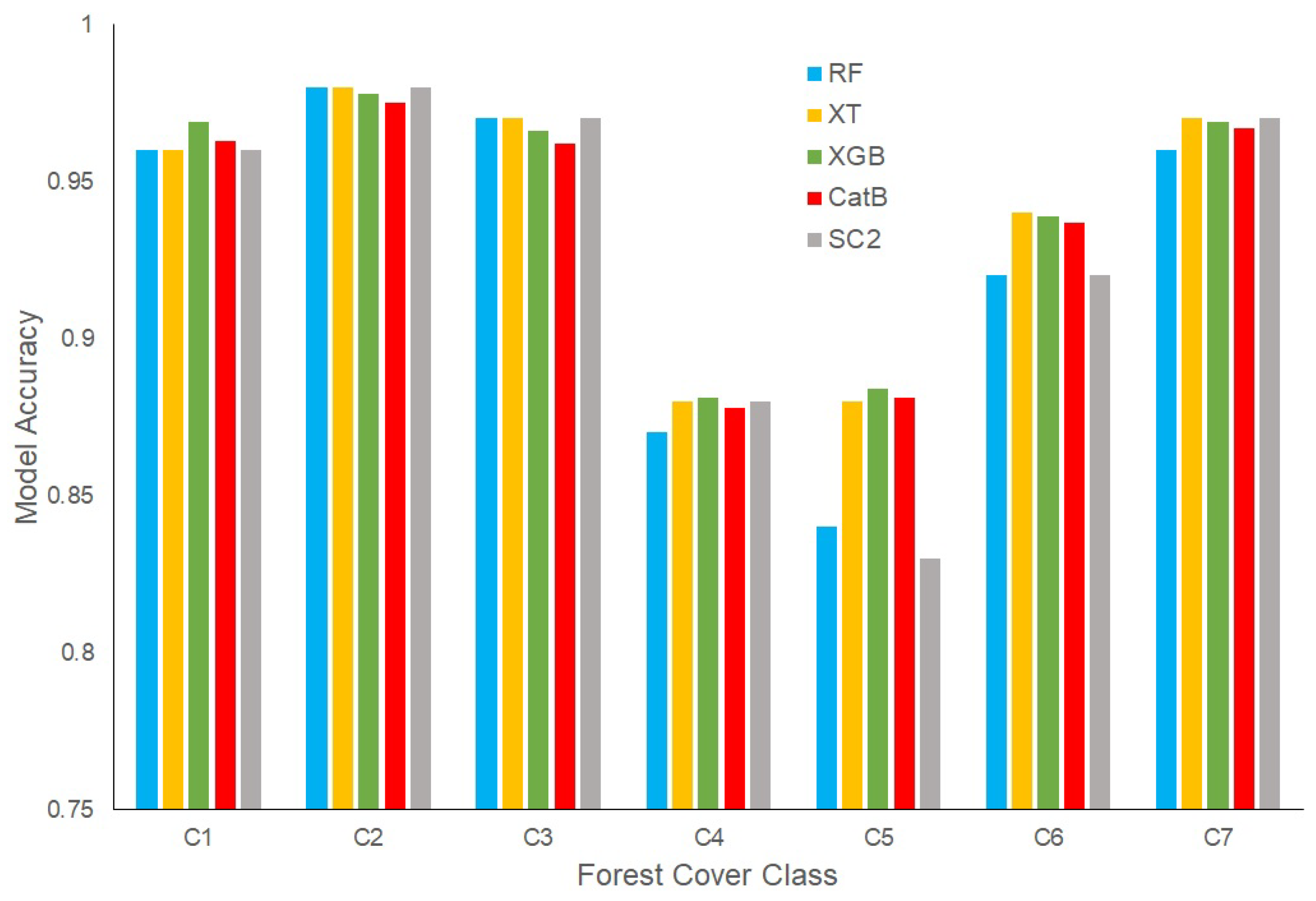
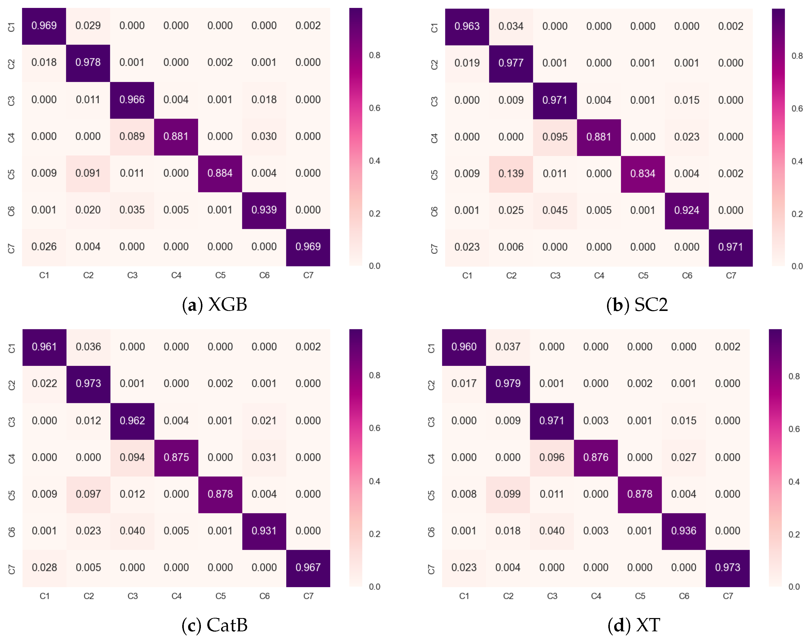
3.3. Accuracy Measures

The overall classification accuracy (macro average) achieved by each of the different models studied here is shown in

Table 3. Accuracy metrics for the implemented models.

Metric	DT	SVR	KNN	RF	XT	Ada	XGB	CatB	SC1	SC2	SC3
acc	0.934	0.913	0.934	0.964	0.968	0.963	0.971	0.967	0.935	0.967	0.940
prec	0.901	0.897	0.897	0.951	0.955	0.952	0.952	0.951	0.898	0.955	0.895
rec	0.898	0.869	0.872	0.928	0.939	0.922	0.941	0.938	0.890	0.932	0.910
F1-score	0.900	0.882	0.884	0.939	0.947	0.936	0.946	0.943	0.893	0.943	0.902

. It can be observed that the highest accuracy over the whole dataset equals 0.97, and is obtained by XGB. This is slightly higher than the accuracy achieved by CatB (0.967), SC3(0.967), and XT (0.968). Even though the optimised RF achieves an accuracy of “only” 0.964, this still surpasses other similar research results, including [41,43]. Despite its higher overall accuracy, XGB exhibits lower precision compared to XT and SC2 and a lower F1 score compared to XT. The lowest overall accuracy is 0.913, achieved by SVM with radial basis kernel (SVR). Nonetheless, this value surpasses accuracy values previously reported in the literature using SVM on the same dataset.

Figure 9 presents the accuracy achieved by the five best-performing models for each of the seven cover types in the dataset. It is clear that all models perform poorly on the C4 and C5 cover types, with the highest accuracy values being 0.881 and 0.884, respectively. Unsurprisingly, these are the two classes with the fewest data samples. However, SC3 and RF performed significantly worse than other models for the C5 cover type. Figure 10 presents the confusion matrix for the XGB, XT, CatB, and SC2 models. It can be observed that the accuracy of estimations for the majority C1 and C2 cover type classes is higher than 0.96 for all models. It is interesting to note that the most prominent misclassifications by all four models are “C5 misclassified as C2” and “C4 misclassified as C3”, and not vice versa.

4. Discussion

This paper proposes a methodology based on Machine Learning (ML) algorithms with automated fine-tuning of the model combined with recursive feature elimination to predict vegetation type from cartographic data. The overall accuracy obtained by the proposed approach using the XGB model on the UCI dataset is $97.1\%$, which surpasses those reported in other studies. For example, Sjöqvist et al. [41] reported an overall accuracy of $94.7\%$, Al Sameer et al. [42] reported $93\%$, and Macmichael and Si [39] achieved an accuracy of $97.01\%$ (the latter using deep learning models).

Considering class-wise accuracy, Figure 10 shows that the four models are slightly overfitted on the majority class, the C2 cover type (283,301 datapoints), achieving the highest accuracy ($97.3$–$97.9\%$). Unsurprisingly, the lowest accuracy ($87.5$–$88.1\%$) corresponds to the minority class, the C4 cover type (2747 datapoints). Somewhat surprisingly, all four models show high accuracy for the C7 cover type, despite its moderate sampling size (20,510 datapoints). Nonetheless, it is important to note that the proposed approach with all four models achieves higher accuracy for the undersampled classes than those reported by previous researchers. For example, while our proposed approach with XGB reaches 88.1%, 88.4%, and 93.9% for classes 4, 5, and 6, respectively, Sjöqvist et al. [41] reported respective accuracy of 77.9%, 77%, and 86%. This comprises a significant improvement. For classification of the C1 and C2 cover types, the same authors reported an accuracy of 93.7% and 96.7%, respectively, while our method using the XGB model achieved 96.9% and 97.8%, respectively. It is notable that using our proposed approach with the RF model used in [41] resulted in an overall accuracy of 96.4%, which is a significant improvement over the results reported in their study.

5. Conclusions

The dynamic behaviour and propagation characteristics of wildfires are highly affected by the type and distribution of the available fuel. Therefore, their accurate estimation is paramount for wildfire model predictions to be of any practical use. To this end, a methodology was proposed in this paper for the accurate classification of vegetation cover type over a landscape from cartographic data. In essence, the proposed methodology is based on state-of-the-art Machine Learning (ML) classifiers combined with automated tuning of their hyperparameters and recursive feature elimination.

The performance of three boosting (AdaB, XGB, CatB), two bagging (RF, XT), and three stacking ensemble models (see Figure 4) were investigated, with XGB outperforming the others. All classifiers were trained and tested on the University of California Irvine (UCI) cover type dataset using five-fold cross-validation, while Bayesian Optimisation was used for the tuning of their hyperparameters. The dataset was subsampled for tuning of the models to cope with imbalance and reduce the required computational effort. A feature importance analysis was carried out to identify the sets of features to be considered by each classifier to achieve its highest overall accuracy. XGB with nine features and tuned with Bayesian Optimisation on a subsampled balanced dataset achieved the highest overall accuracy at $97.1\%$. This is higher than previous values reported in the literature. Because training was performed on the full rather than the subsampled dataset, the class-wise accuracy was slightly lower for the undersampled cover type classes, as expected. Nonetheless, these values were significantly higher than those previously reported in the literature for the same dataset. It is interesting to note that the resulting class-wise accuracies are more uniform than those reported by other authors, which suggests that the proposed method is effective at handling imbalanced datasets. This may be thanks to the automated tuning of the model’s hyperparameters using a balanced subsampled dataset.

While the results obtained here show that the proposed approach is accurate at predicting vegetation cover type over a landscape from cartographic data, and therefore the fuel type and distribution, it goes without saying that the trained models would work accurately only in the region where they were trained and tested. It is hypothesised that the generalisability of the classifier can be enhanced by a number of methods, including: removing region-specific features such as wilderness; emphasising general features such as slope, hillshade indices, and parameterised soil type; incorporating climatic variables such as temperature and precipitation; and training on larger datasets covering different regions. Potential lines of future work might include investigating the feasibility, accuracy, and generalisability of fusion between classifiers based on cartographic data and vegetation cover type predictors based on remote sensing. In order to foster and facilitate adoption, it is important to work on the integration of vegetation cover type classifiers such as the one proposed in this paper into existing fire hazard/danger systems.

References

1. Giglio, L.; Boschetti, L.; Roy, D.P.; Humber, M.L.; Justice, C.O. The Collection 6 MODIS burned area mapping algorithm and product. Remote Sens. Environ. 2018, 217, 72–85. [Google Scholar] [CrossRef]
2. Jurvélius, M. Forest Fires (Prediction, Prevention, Preparedness and Suppression). In Encyclopedia of Forest Sciences; Elsevier: Amsterdam, The Netherlands, 2004; pp. 334–339. [Google Scholar] [CrossRef]
3. Bond, W.J.; Keeley, J.E. Fire as a global ‘herbivore’: The ecology and evolution of flammable ecosystems. Trends Ecol. Evol. 2005, 20, 387–394. [Google Scholar] [CrossRef]
4. Innocente, M.S.; Grasso, P. Self-organising swarms of firefighting drones: Harnessing the power of collective intelligence in decentralised multi-robot systems. J. Comput. Sci. 2019, 34, 80–101. [Google Scholar] [CrossRef]
5. Coogan, S.C.; Robinne, F.N.; Jain, P.; Flannigan, M.D. Scientists’ warning on wildfire—A Canadian perspective. Can. J. For. Res. 2019, 49, 1015–1023. [Google Scholar] [CrossRef] [Green Version]
6. Jain, P.; Coogan, S.C.; Subramanian, S.G.; Crowley, M.; Taylor, S.; Flannigan, M.D. A review of machine learning applications in wildfire science and management. Environ. Rev. 2020, 28, 478–505. [Google Scholar] [CrossRef]
7. Scott, J.H.; Reinhardt, E.D. Assessing Crown Fire Potential by Linking Models of Surface and Crown Fire Behavior; Technical Report; U.S. Department of Agriculture: Fort Collins, CO, USA, 2001. [CrossRef] [Green Version]
8. Finney, M.A. FARSITE: Fire Area Simulator-Model Development and Evaluation; Technical Report; U.S. Department of Agriculture: Fort Collins, CO, USA, 1998. [CrossRef]
9. Linn, R.; Reisner, J.; Colman, J.J.; Winterkamp, J. Studying wildfire behavior using FIRETEC. Int. J. Wildland Fire 2002, 11, 233. [Google Scholar] [CrossRef]
10. Mell, W.; Jenkins, M.A.; Gould, J.; Cheney, P. A physics-based approach to modelling grassland fires. Int. J. Wildland Fire 2007, 16, 1. [Google Scholar] [CrossRef]
11. Grasso, P.; Innocente, M.S. A two-dimensional reaction-advection-diffusion model of the spread of fire in wildlands. In Advances in Forest Fire Research 2018; Imprensa da Universidade de Coimbra: Coimbra, Portugal, 2018; pp. 334–342. [Google Scholar] [CrossRef] [Green Version]
12. Grasso, P.; Innocente, M.S. Physics-based model of wildfire propagation towards faster-than-real-time simulations. Comput. Math. Appl. 2020, 80, 790–808. [Google Scholar] [CrossRef]
13. Kim, Y.H.; Bettinger, P.; Finney, M. Spatial optimization of the pattern of fuel management activities and subsequent effects on simulated wildfires. Eur. J. Oper. Res. 2009, 197, 253–265. [Google Scholar] [CrossRef]
14. Arroyo, L.A.; Pascual, C.; Manzanera, J.A. Fire models and methods to map fuel types: The role of remote sensing. For. Ecol. Manag. 2008, 256, 1239–1252. [Google Scholar] [CrossRef] [Green Version]
15. Martell, D.L. A Review of Recent Forest and Wildland Fire Management Decision Support Systems Research. Curr. For. Rep. 2015, 1, 128–137. [Google Scholar] [CrossRef] [Green Version]
16. Ausonio, E.; Bagnerini, P.; Ghio, M. Drone Swarms in Fire Suppression Activities: A Conceptual Framework. Drones 2021, 5, 17. [Google Scholar] [CrossRef]
17. Campbell, M.J.; Page, W.G.; Dennison, P.E.; Butler, B.W. Escape Route Index: A Spatially-Explicit Measure of Wildland Firefighter Egress Capacity. Fire 2019, 2, 40. [Google Scholar] [CrossRef] [Green Version]
18. Kato, A.; Moskal, L.M.; Schiess, P.; Swanson, M.E.; Calhoun, D.; Stuetzle, W. Capturing tree crown formation through implicit surface reconstruction using airborne lidar data. Remote Sens. Environ. 2009, 113, 1148–1162. [Google Scholar] [CrossRef]
19. Yebra, M.; Quan, X.; Riaño, D.; Larraondo, P.R.; van Dijk, A.I.; Cary, G.J. A fuel moisture content and flammability monitoring methodology for continental Australia based on optical remote sensing. Remote Sens. Environ. 2018, 212, 260–272. [Google Scholar] [CrossRef]
20. Engelstad, P.S.; Falkowski, M.; Wolter, P.; Poznanovic, A.; Johnson, P. Estimating Canopy Fuel Attributes from Low-Density LiDAR. Fire 2019, 2, 38. [Google Scholar] [CrossRef] [Green Version]
21. Rao, K.; Williams, A.P.; Flefil, J.F.; Konings, A.G. SAR-enhanced mapping of live fuel moisture content. Remote Sens. Environ. 2020, 245, 111797. [Google Scholar] [CrossRef]
22. Marino, E.; Tomé, J.L.; Hernando, C.; Guijarro, M.; Madrigal, J. Transferability of Airborne LiDAR Data for Canopy Fuel Mapping: Effect of Pulse Density and Model Formulation. Fire 2022, 5, 126. [Google Scholar] [CrossRef]
23. Vorster, A.G.; Evangelista, P.H.; Stovall, A.E.L.; Ex, S. Variability and uncertainty in forest biomass estimates from the tree to landscape scale: The role of allometric equations. Carbon Balance Manag. 2020, 15, 8. [Google Scholar] [CrossRef]
24. Anderson, K.E.; Glenn, N.F.; Spaete, L.P.; Shinneman, D.J.; Pilliod, D.S.; Arkle, R.S.; McIlroy, S.K.; Derryberry, D.R. Estimating vegetation biomass and cover across large plots in shrub and grass dominated drylands using terrestrial lidar and machine learning. Ecol. Indic. 2018, 84, 793–802. [Google Scholar] [CrossRef]
25. Hartley, R.J.L.; Davidson, S.J.; Watt, M.S.; Massam, P.D.; Aguilar-Arguello, S.; Melnik, K.O.; Pearce, H.G.; Clifford, V.R. A Mixed Methods Approach for Fuel Characterisation in Gorse (Ulex europaeus L.) Scrub from High-Density UAV Laser Scanning Point Clouds and Semantic Segmentation of UAV Imagery. Remote Sens. 2022, 14, 4775. [Google Scholar] [CrossRef]
26. Zheng, Y.; Jia, W.; Wang, Q.; Huang, X. Deriving Individual-Tree Biomass from Effective Crown Data Generated by Terrestrial Laser Scanning. Remote Sens. 2019, 11, 2793. [Google Scholar] [CrossRef] [Green Version]
27. Carpenter, J.; Jung, J.; Oh, S.; Hardiman, B.; Fei, S. An Unsupervised Canopy-to-Root Pathing (UCRP) Tree Segmentation Algorithm for Automatic Forest Mapping. Remote Sens. 2022, 14, 4274. [Google Scholar] [CrossRef]
28. Hoffmann, C.W.; Usoltsev, V.A. Tree-crown biomass estimation in forest species of the Ural and of Kazakhstan. For. Ecol. Manag. 2002, 158, 59–69. [Google Scholar] [CrossRef]
29. Fogarty, L.G.; Pearce, H.G. Draft field guides for determining fuel loads and biomassin New Zealand vegetation types. Fire Technol. Transf. Note 2000, 21, 2–15. [Google Scholar]
30. Crespo-Peremarch, P.; Ruiz, L.; Balaguer-Beser, A. A comparative study of regression methods to predict forest structure and canopy fuel variables from LiDAR full-waveform data. Rev. Teledetección 2016, 27–40. [Google Scholar] [CrossRef] [Green Version]
31. Chuvieco, E.; Riaño, D.; Wagtendok, J.V.; Morsdof, F. Fuel Loads and Fuel Type Mapping. In Series in Remote Sensing; World Scientific: Singapore, 2003; pp. 119–142. [Google Scholar] [CrossRef]
32. Lasaponara, R.; Lanorte, A. Remotely sensed characterization of forest fuel types by using satellite ASTER data. Int. J. Appl. Earth Obs. Geoinf. 2007, 9, 225–234. [Google Scholar] [CrossRef]
33. Pearce, H.; Anderson, W.; Fogarty, L.; Todoroki, C.; Anderson, S. Linear mixed-effects models for estimating biomass and fuel loads in shrublands. Can. J. For. Res. 2010, 40, 2015–2026. [Google Scholar] [CrossRef]
34. Li, Y.; Li, C.; Li, M.; Liu, Z. Influence of Variable Selection and Forest Type on Forest Aboveground Biomass Estimation Using Machine Learning Algorithms. Forests 2019, 10, 1073. [Google Scholar] [CrossRef] [Green Version]
35. Luo, M.; Wang, Y.; Xie, Y.; Zhou, L.; Qiao, J.; Qiu, S.; Sun, Y. Combination of Feature Selection and CatBoost for Prediction: The First Application to the Estimation of Aboveground Biomass. Forests 2021, 12, 216. [Google Scholar] [CrossRef]
36. Blackard, J.A.; Dean, D.J. Comparative accuracies of artificial neural networks and discriminant analysis in predicting forest cover types from cartographic variables. Comput. Electron. Agric. 1999, 24, 131–151. [Google Scholar] [CrossRef] [Green Version]
37. Pierce, A.D.; Farris, C.A.; Taylor, A.H. Use of random forests for modeling and mapping forest canopy fuels for fire behavior analysis in Lassen Volcanic National Park, California, USA. For. Ecol. Manag. 2012, 279, 77–89. [Google Scholar] [CrossRef]
38. Patil, P.R.; Sivagami, M. Forest Cover Classification Using Stacking of Ensemble Learning and Neural Networks. In Advances in Intelligent Systems and Computing; Springer: Singapore, 2020; pp. 89–102. [Google Scholar] [CrossRef]
39. Macmichael, D.; Si, D. Addressing Forest Management Challenges by Refining Tree Cover Type Classification with Machine Learning Models. In Proceedings of the 2017 IEEE International Conference on Information Reuse and Integration (IRI), Hong Kong, China, 4–6 August 2017; IEEE: Piscataway, NJ, USA, 2017. [Google Scholar] [CrossRef]
40. Samat, A.; Li, E.; Du, P.; Liu, S.; Xia, J. GPU-Accelerated CatBoost-Forest for Hyperspectral Image Classification Via Parallelized mRMR Ensemble Subspace Feature Selection. IEEE J. Sel. Top. Appl. Earth Obs. Remote Sens. 2021, 14, 3200–3214. [Google Scholar] [CrossRef]
41. Sjöqvist, H.; Längkvist, M.; Javed, F. An Analysis of Fast Learning Methods for Classifying Forest Cover Types. Appl. Artif. Intell. 2020, 34, 691–709. [Google Scholar] [CrossRef]
42. Al Sameer, M.M.; Prasanth, T.; Anuradha, R. Rapid Forest Cover Detection Using Ensemble Learning. In Lecture Notes in Electrical Engineering; Springer: Singapore, 2021; pp. 181–190. [Google Scholar] [CrossRef]
43. Kumar, A.; Sinha, N. Classification of Forest Cover Type Using Random Forests Algorithm. In Advances in Data and Information Sciences; Springer: Singapore, 2020; pp. 395–402. [Google Scholar] [CrossRef]
44. Kumar, P.P.; Bai, V.M.A.; Nair, G.G. An efficient classification framework for breast cancer using hyper parameter tuned Random Decision Forest Classifier and Bayesian Optimization. Biomed. Signal Process. Control 2021, 68, 102682. [Google Scholar] [CrossRef]
45. Subasree, S.; Sakthivel, N.; Tripathi, K.; Agarwal, D.; Tyagi, A.K. Combining the advantages of radiomic features based feature extraction and hyper parameters tuned RERNN using LOA for breast cancer classification. Biomed. Signal Process. Control 2022, 72, 103354. [Google Scholar] [CrossRef]
46. Wang, Y.; Zhang, H.; Zhang, G. cPSO-CNN: An efficient PSO-based algorithm for fine-tuning hyper-parameters of convolutional neural networks. Swarm Evol. Comput. 2019, 49, 114–123. [Google Scholar] [CrossRef]
47. ArcGIS—Wilderness Areas in the United States. 2023. Available online: https://www.arcgis.com/apps/mapviewer/index.html?layers=52c7896cdfab4660a595e6f6a7ef0e4d (accessed on 3 December 2022).
48. Cortes, C.; Vapnik, V. Support-vector networks. Mach. Learn. 1995, 20, 273–297. [Google Scholar] [CrossRef]
49. Aizerman, M.A.; Braverman, E.A.; Rozonoer, L. Theoretical Foundations of the Potential Function Method in Pattern Recognition Learning. Autom. Remote Control 1964, 25, 821–837. [Google Scholar]
50. Breiman, L.; Friedman, J.H.; Olshen, R.A.; Stone, C.J. Classification And Regression Trees; Routledge: England, UK, 2017. [Google Scholar] [CrossRef]
51. Caie, P.D.; Dimitriou, N.; Arandjelović, O. Precision medicine in digital pathology via image analysis and machine learning. In Artificial Intelligence and Deep Learning in Pathology; Elsevier: Amsterdam, The Netherlands, 2021; pp. 149–173. [Google Scholar] [CrossRef]
52. Geurts, P.; Ernst, D.; Wehenkel, L. Extremely randomized trees. Mach. Learn. 2006, 63, 3–42. [Google Scholar] [CrossRef] [Green Version]
53. Breiman, L. Stacked regressions. Mach. Learn. 1996, 24, 49–64. [Google Scholar] [CrossRef] [Green Version]
54. Friedman, J.H. Greedy function approximation: A gradient boosting machine. Ann. Stat. 2001, 29, 1189–1232. [Google Scholar] [CrossRef]
55. Gale, M.G.; Cary, G.J.; Dijk, A.I.V.; Yebra, M. Forest fire fuel through the lens of remote sensing: Review of approaches, challenges and future directions in the remote sensing of biotic determinants of fire behaviour. Remote Sens. Environ. 2021, 255, 112282. [Google Scholar] [CrossRef]
56. Hancock, J.T.; Khoshgoftaar, T.M. CatBoost for big data: An interdisciplinary review. J. Big Data 2020, 7, 1–45. [Google Scholar] [CrossRef] [PubMed]
57. Chen, T.; Guestrin, C. XGBoost. In Proceedings of the 22nd ACM SIGKDD International Conference on Knowledge Discovery and Data Mining, San Francisco, CA, USA, 13–17 August 2016; ACM: New York, NY, USA, 2016. [Google Scholar] [CrossRef] [Green Version]
58. Cover, T. Estimation by the nearest neighbor rule. IEEE Trans. Inf. Theory 1968, 14, 50–55. [Google Scholar] [CrossRef] [Green Version]
59. Freund, Y.; Schapire, R.E. A Decision-Theoretic Generalization of On-Line Learning and an Application to Boosting. J. Comput. Syst. Sci. 1997, 55, 119–139. [Google Scholar] [CrossRef] [Green Version]
60. Schapire, R.E. A brief introduction to boosting. In Proceedings of the Sixteenth International Joint Conference on Artificial Intelligence, Stockholm, Sweden, 31 July–6 August 1999. [Google Scholar]
61. Prokhorenkova, L.; Gusev, G.; Vorobev, A.; Dorogush, A.V.; Gulin, A. CatBoost: Unbiased Boosting with Categorical Features. In Proceedings of the 32nd International Conference on Neural Information Processing Systems, Montreal, QC, Canada, 3–8 December 2018; NIPS’18. Curran Associates Inc.: Red Hook, NY, USA, 2018; pp. 6639–6649. [Google Scholar]
62. Tao, H.; Habib, M.; Aljarah, I.; Faris, H.; Afan, H.A.; Yaseen, Z.M. An intelligent evolutionary extreme gradient boosting algorithm development for modeling scour depths under submerged weir. Inf. Sci. 2021, 570, 172–184. [Google Scholar] [CrossRef]
63. Brochu, E.; Cora, V.; de Freitas, N. A Tutorial on Bayesian Optimization of Expensive Cost Functions, with Application to Active User Modeling and Hierarchical Reinforcement Learning. arXiv 2010, arXiv:1012.2599. [Google Scholar]
64. Wu, J.; Chen, X.Y.; Zhang, H.; Xiong, L.D.; Lei, H.; Deng, S.H. Hyperparameter Optimization for Machine Learning Models Based on Bayesian Optimizationb. J. Electron. Sci. Technol. 2019, 17, 26–40. [Google Scholar] [CrossRef]
65. Nguyen, V. Bayesian Optimization for Accelerating Hyper-Parameter Tuning. In Proceedings of the 2019 IEEE Second International Conference on Artificial Intelligence and Knowledge Engineering (AIKE), Sardinia, Italy, 3–5 June 2019; IEEE: Piscataway, NJ, USA, 2019. [Google Scholar] [CrossRef]
66. Akiba, T.; Sano, S.; Yanase, T.; Ohta, T.; Koyama, M. Optuna: A Next-generation Hyperparameter Optimization Framework. In Proceedings of the 25th ACM SIGKDD International Conference on Knowledge Discovery & Data Mining, Anchorage, AK, USA, 4–8 August 2019; ACM: New York, NY, USA, 2019. [Google Scholar] [CrossRef]
67. Pedregosa, F.; Varoquaux, G.; Gramfort, A.; Michel, V.; Thirion, B.; Grisel, O.; Blondel, M.; Prettenhofer, P.; Weiss, R.; Dubourg, V.; et al. Scikit-learn: Machine Learning in Python. J. Mach. Learn. Res. 2011, 12, 2825–2830. [Google Scholar]
68. XGBoost Project. 2022. Available online: https://github.com/dmlc/xgboost) (accessed on 3 December 2022).
69. CatBoost. 2022. Available online: https://catboost.ai/ (accessed on 3 December 2022).
70. Hossin, M.; Sulaiman, M.N. A Review on Evaluation Metrics for Data Classification Evaluations. Int. J. Data Min. Knowl. Manag. Process 2015, 5, 1–11. [Google Scholar] [CrossRef]
Figure 1. Study area location map: Roosevelt National Forest wilderness areas (extracted and modified from [47]).
Fire 06 00076 g001
Figure 2. Feature correlation matrix (Pearson), with r below and p-value above the diagonal.
Fire 06 00076 g002
Figure 3. Pairwise distribution and relationship of features in the dataset.
Fire 06 00076 g003
Figure 4. Structure used for the Stacked Classification models.
Fire 06 00076 g004
Figure 5. Visualisation of the hyperparameter optimisation procedure for the DT algorithm.
Fire 06 00076 g005
Figure 6. Visualisation of the hyperparameter optimisation procedure for the XGB algorithm. Note that notation Ae-B is meant to represent A × 10 B in scientific notation.
Fire 06 00076 g006
Figure 7. Relative importance of features.
Fire 06 00076 g007
Figure 8. Accuracy during recursive feature elimination test.
Fire 06 00076 g008
Figure 9. Accuracy of different classifiers for each cover class.
Fire 06 00076 g009
Figure 10. Confusion matrix of the four best-performing classifiers for predicted cover type classes.
Fire 06 00076 g010