Study of Fuel-Smoke Dynamics in a Prescribed Fire of Boreal Black Spruce Forest through Field-Deployable Micro Sensor Systems

Abstract

Understanding the combustion dynamics of fuels, and the generation and propagation of smoke in a wildland fire, can inform short-range and long-range pollutant transport models, and help address and mitigate air quality concerns in communities. Smoldering smoke can cause health issues in nearby valley bottoms, and can create hazardous road conditions due to low-visibility. We studied near-field smoke dynamics in a prescribed fire of 3.4 hectares of land in a boreal black spruce forest in central Alberta. Smoke generated from the fire was monitored through a network of five field-deployable micro sensor systems. Sensors were placed within 500–1000 m of the fire area at various angles in downwind. Smoke generated from flaming and smoldering combustions showed distinct characteristics. The propagation rates of flaming and smoldering smoke, based on the fine particulate (PM_2.5) component, were 0.8 and 0.2 m/s, respectively. The flaming smoke was characterized by sharp rise of PM_2.5 in air with concentrations of up to 940 µg/m³, followed by an exponential decay with a half-life of ~10 min. Smoldering combustion related smoke contributed to PM_2.5 concentrations above 1000 µg/m³ with slower decay half-life of ~18 min. PM_2.5 emissions from the burn area during flaming and smoldering phases, integrated over the combustion duration of 2.5 h, were ~15 and ~16 kilograms, respectively, as estimated by our mass balance model.

1. Introduction

Smoke created from wildland fires causes air quality concerns for communities across North America. Depending on the location, duration, and volume of wildland fires, public health can be subject to moderate to severe risks at nearby and/or distant locations for short to extended periods. Emissions from the burning of biomass in wildland areas primarily generate carbon dioxide (CO₂), carbon monoxide (CO), particulate matters (PM), volatile organic compounds (VOC), nitrous oxides (NO_x), ammonia (NH₃), small amounts of sulphur dioxide (SO₂), and methane (CH₄) [1,2]. It has been reported that almost 90% of carbon emitted from wildland fires are of the form of CO₂ [3,4,5]. The emitted CO₂ is estimated to contribute up to 40 ppm of the global CO₂ budget [1]. VOCs emitted from wildland fire, although a small fraction of the total emission, may be associated with adverse health effects and can be a source of ozone formation in warmer summer conditions in the presence of solar radiation. Fine particulate matter with aerodynamic diameters of less than 2.5 µm (PM_2.5) emitted from wildland fires can enhance the ambient concentration levels by orders of magnitude, and is generally regarded as the most important concern from wildfire smoke [6]. In Alberta, the last five years’ average of wildland fires is above 200,000 hectares/year, with 883,411 hectares of land burned by 989 fires in the year of 2019 [7]. These fires frequently cause elevated levels of particulate matter at population centres that are well above levels recommended by the Alberta Ambient Air Quality Guideline [8,9].

Fuel types in a typical boreal forest are categorized as canopy, shrub, non-woody vegetation, woody, litter-lichen-moss, and ground fuels [10,11]. Fire behaviour and emission factors during a wildland fire strongly depend on the distribution of fuel types in the fuel-bed, fire-weather, and atmospheric conditions. Combustion of fuels of lower moisture content and larger surface to volume ratio (often less than 1 cm in diameter) produce a significant initial flaming phase where fuel temperature rises from 500 °C to 1900 °C [11,12,13]. Plants and organic fuels release volatile combustible gases during this phase and create a sustained fire front that spreads with the wind. Flaming combustion is succeeded by a residual smoldering combustion (RSC) phase when emissions of combustible gases are reduced, with a subsequent reduction of temperature and fire spread rate [14,15]. Large diameter woody fuels, duff, organic soils, and rotten logs are typical examples where fuel consumption occurs predominantly by smoldering. The smoldering combustion of organic soils (peat) and duff in Black Spruce dominated Boreal peatlands is a slower moving process compared to flaming [16]. Relative humidity, temperature, and wind speed also play roles in the dynamics of combustion and the spread of fires. In Boreal peatlands under normal moisture conditions, low severity peat burns typically release 2–3 kg C/m² during wildfires in the smoldering phase, a value that increases to 10–85 kg C/m² under dry conditions [17].

Smoke generated by the flaming and smoldering phases of fire differ significantly in their characteristics. The flaming phase is characterized by higher combustion efficiency, typically measured as modified combustion efficiency (MCE) [3]. Smoke plumes generated during the flaming phase are very buoyant due to their high temperature and are lofted to higher atmospheric levels, where they are responsible for long range transport of pollutants [18,19,20]. Intense heat induced aerodynamics in the flaming phase may also result in modification of the local meteorological wind and temperature fields [21]. The smoldering phase of combustion is characterized by a lower MCE that produces higher fractions of CO, organic aerosols (OA), CH₄, and non-methane organic compounds (NMOC) [22]. Smoke generated during smoldering is highly visible due to higher content of condensed vapor and particulates [11]. Absence of flaming induced intense heat results in smoke propagating near ground level, sometimes concentrating on valley bottoms or depressions. Smoke from smoldering has been attributed to air quality concerns and severe low-visibility traffic hazards [11,23,24].

There are knowledge gaps in understanding fuel consumption during flaming and smoldering combustion for different types of fuels. This results in large uncertainties in estimating effective emission factors for individual species in wildland fire generated smoke [3,25]. Observation of smoke from airborne and tower based measurements exclude the smoke propagation near the ground level. Ground level measurements, especially in near-field regions of a wildland fire, are inherently challenging due to logistical constraints. Apart from safety involved in accessing to the close vicinity of an active fire area, operational constraints (e.g., requirements of power and controlled ambience for equipment, installation, safety of operation) of most air-pollutant analyzers prohibit their deployment in near-field wildland fire studies. Smoke generated from smoldering, in many cases, are analyzed in laboratory environments to supplement field measurements [3]. As a result, although the evolution of flaming and smoldering phases of fire are extensively reported in literature, smoke dynamics during and immediately after the spread of a firefront in relation to fuel types are not well understood. Better identification and characterization of flaming and smoldering smoke can enhance the modeling of wildland fire smoke propagations in micro level as well as macro level long range transports [25].

Recent developments in low-cost air monitoring sensors have opened up new possibilities of expanding the coverage of air monitoring to remote areas in a cost-effective approach [8,26]. These sensor systems, typically of the size of a shoebox, have energy consumptions of 5–10 watts, and cost significantly less than conventional analyzer systems. In this paper, we describe the deployment of custom-built low-footprint field deployable air monitoring micro systems in a prescribed fire of boreal forest in central Alberta, undertaken in May 2019, to study fuel–smoke dynamics through near field real-time measurements. Our analysis of PM_2.5 measurements by a network of five micro sensor systems identifies and characterizes smoke from both flaming and smoldering phases of the fire. We show that smoke intensity can have strong spatial distributions, and smoke from smoldering origin may have a sustaining presence in the near-field regions of a fire. We demonstrate the practical use of low-cost sensor systems to parameterize fine particulate matter emissions from flaming and smoldering phases of combustion estimated through a mass balance model.

2. Materials and Methods

2.1. Study Area

The prescribed fire was conducted on 3.4 hectares of land on boreal forest in central Alberta (Pelican Mountain unit 5). The forest area was predominantly covered by black spruce, with canopy closure of over 50%. The ground consisted of thick organic soil covered mostly with feathermosses with a minor presence of Sphagnum mosses. A well-mixed boundary layer with predominant southerly winds at speeds varying in ranges of 5 km/h up to 23 km/h (10 m above ground level open wind speed) with occasional gusts were measured by a sonic anemometer placed in the south of the area. The timing of the fire was late afternoon on 11 May 2019. Fire was ignited through a helicopter-borne torch along the ignition line at the south perimeter of the area. The fire behavior and the spread to the north direction was recorded through in-situ measurements. Details can be found in Thompson et al. [27]. Five micro-stations were deployed at downwind locations of the prescribed fire zone. Four micro-stations were placed approximately at distances of 500 m from unit 5 at northeast, north, northwest, and west-northwest directions, respectively. One micro-station was placed at approximately 1 km distance in northwest direction. Micro-stations were transported to deployment sites through helicopters, and exact locations of deployments were subject to site accessibility. All micro-stations were deployed approximately twenty-four hours before the prescribed fire to monitor the background air quality in the area. Figure 1 shows the micro-station deployment locations.

2.2. Micro Sensor Systems

Smoke dynamics during and after the prescribed fire was monitored by a network of five field deployable, low-footprint, sensor equipped micro air monitoring systems. These systems, referred to as micro-stations in this paper, were custom made by Alberta Environment and Parks for emergency deployments and remote area monitoring [8]. The shoebox-sized micro-stations can be conveniently transported and placed on tripods at remote forest locations. They are designed to run on solar power, with a battery back-up time of up to 72 h. The micro-stations were equipped with sensors for detection of airborne particulate matter (PM) with aerodynamic diameters of up to 1, 2.5, and 10 µm (PM₁, PM_2.5, and PM₁₀, respectively). Some micro-stations were also equipped with additional sensors for monitoring of ozone, carbon dioxide, formaldehyde, and volatile organic compound (VOC). All micro-stations had ambient temperature and humidity sensors. Plantower PMS6003 and QS1005 sensors were used for PM detection. These sensors have a manufacturer specified consistency error of ±10 µg/m³ with resolutions of 1 µg/m³. Aeroqual SM50 ozone sensors were used with a resolution of 12-bit for analog signals. Sensor deployment details are provided in

Table 1. Micro-station deployment details. Distances are measured from an assumed center location of the fire-area, shown in Figure 1.

Micro-Station Serial	Location	Latitude	Longitude	Distance (m)
µS 303–100	North	55.7219	–113.573	415
µS 303–200	NW	55.7214	–113.578	474
µS 303–300	NE	55.7211	–113.566	567
µS 401–100	WNW	55.7296	–113.581	529
µS 401–200	NW	55.7245	–113.584	973

.

2.3. Data Analysis and Models

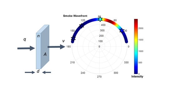
2.3.1. Smoke Propagation

We used a mass balance model to describe the smoke dynamics and its relations to the types of fuel consumption. Smoke dynamics were monitored through measurements of PM_2.5 at the five locations where micro-stations were deployed. Time-series concentration profiles showed occurrences of three smoke wavefronts when sharp enhancements in PM_2.5 concentrations were recorded simultaneously at two or more stations. Decrease of PM_2.5 concentrations at varying rates of decay followed the three smoke wavefronts at all micro-station locations.

To understand the time-series PM_2.5 concentration profile in relation to smoke dynamics, we start with equating the influx and outflow of PM_2.5 at an imaginary vertical box in a direction perpendicular to smoke propagation at a measurement location (see Figure 2). Neglecting transverse dispersion, and assuming that excess PM_2.5 mass accumulates with uniform density along an effective length of d, the dynamic balance can be represented as,

$$\mathsf{\Delta }nAd=(qA-nAv)\mathsf{\Delta }t,$$

(1)

where,

• q = flux of PM_2.5 in the incoming smoke (µg/m²/s),
• v = propagation velocity of smoke plume wavefront (m/s),
• n = effective concentration of PM_2.5 within the vertical three dimensional box (µg/m³),
• Δn = n(t₂) − n(t₁) = increase in PM_2.5 concentration within the box during an interval Δt (µg/m³),
• Δt = t₂ − t₁ = time interval (s)
• A = area of the imaginary cross section at the measurement location (m²), and
• d = effective length of virtual box where excess PM_2.5 distribution is considered to be uniform (m).

The left hand side of Equation (1) represents total increase of mass within an imaginary air volume with cross section of A and a depth of d beginning from the measurement location to downwind. The two terms in the right hand side represents the inflow and outflow of PM_2.5 mass during a time interval Δt, respectively. At a steady state condition, the two terms in the right hand side would cancel each other, and the resulting increase in concentration will be zero.

Equation (1) leads to the differential equation,

$$\frac{dn\left(t\right)}{dt}=\frac{1}{d}(q-n\left(t\right)v),$$

(2)

Equation (2) can be solved as [28],

$$n\left(t\right)=n_0{e}^{-\frac{v}{d}t}+\frac{q}{v}(1-e^{-\frac{v}{d}t}),$$

(3)

where, $n=n_0$ at time, $t=0$.

For instances when a smoke wavefront has just past through a micro-station location, $q\left(t\right)=0$, and Equation (3) converts to,

$$n\left(t\right)=n_0{e}^{-\frac{v}{d}t}.$$

(4)

The rate constant term v/d in Equation (4) in units of (second)⁻¹ is a measure of propagation speed of smoke wavefronts on a relative scale. The corresponding half-life of smoke decay is given as:

$$T_{\raisebox{1ex}{$1$}\!\left/ \!\raisebox{-1ex}{$2$}\right.}=\frac{\ln 2}{v/d}.$$

(5)

2.3.2. Gaussian Profiling of Smoke Dispersion

Smoke generated from the prescribed fire at Pelican Mountain unit 5 were monitored through four micro-stations deployed at distances of 500 m and a fifth micro-station further downwind at 1 km. The four micro-stations deployed in near-field region cover an arc angle of 128 degrees in the downwind and collectively captured the entire smoke plume. Data collected by these four micro-stations can thus be used to simulate the plume profile.

For each wavefront, a set of peak PM_2.5 concentrations at the four locations were fit into a Gaussian profile to simulate the smoke distribution along the arc length of the propagation wavefront. Arc radius for the Gaussian fit was taken as the average distance of individual micro-stations from an approximate center location of the burn area (see Figure 1). Distances were calculated from geospatial coordinates. The smoke wavefront analysis thus assumed that the observation points are equidistant from the centre location of the fire area and all of the smoke originated from this location. Peak PM_2.5 concentrations measured at the three distinct smoke wavefronts where two or more micro-stations observed elevated levels were then fit into Gaussian function in a polar distribution. Details are given in Appendix A.

2.3.3. PM_2.5 Emission from Combustion of Fuels

Emission of PM_2.5 mass from the fire was estimated through calculation of mass flow at ground level during propagation of the smoke-waves. Ground level flow of PM_2.5 mass at peak intensity of a smoke-wave (wavefront) was calculated as:

$$Q={{\displaystyle \int }}_{l_1}^{l_2}vn(l)Hdl,$$

(6)

where,

• Q = flow of PM_2.5 at the wavefront (µg/s),
• v = smoke propagation velocity (m/s),
• l = length along the arc of the smoke wavefront (m), l₁ and l₂ are the lower and upper limits describing the smoke wavefront distribution,
• n(l) = PM_2.5 density as a function of arc length (µg/m³),
• H = height of smoke plume from ground.

Total PM_2.5 mass in a smoke-wave can then be calculated as:

$$M_{P{M}_{2.5}}=\frac{Q}{n{\left(t\right)}_{max}}{{\displaystyle \int }}_{t_0}^{t_0+T}n(t)dt,$$

(7)

where,

• M_PM2.5 = mass of PM_2.5 in smoke-wave,
• n(t) = PM_2.5 density as a function of time (µg/m³),
• n(t)_max = peak PM_2.5 intensity at the smoke-wave (µg/m³),
• t₀ = onset of smoke-wave detection at sensor location, and
• T = duration of smoke-wave recorded at sensor location (s).

Calculation of PM_2.5 mass in smoke-waves and their relation to overall emissions from combustion of fuels are provided in Appendix B.

3. Results

3.1. Background Ambient Conditions

Background ambient conditions were measured for approximately twenty-four hours before the fire. Concentrations of PM_2.5 were low throughout the period of background measurements. Measured PM_2.5 concentrations for the five micro-stations are shown in Figure 3. Some occasional spikes of PM_2.5 concentrations for up to 35 µg/m³ were recorded for the micro-station located at the north of unit 5. PM_2.5 levels recorded at other locations were negligible, and below the sensor minimum detection level (MDL) in most of the cases. The overall background PM_2.5 level corresponds to good air quality conditions on the site with no nearby emission sources.

Ambient temperature and relative humidity at all micro-station locations showed typical diurnal cycles. Overnight temperature reduced to around 0 °C with gradually heating up to 25 °C in the early afternoon. Relative humidity reached above 90% around dawn and went down towards 15% in the early afternoon. At the time of the fire, air temperature and humidity were in the shoulder regions of faster evening period changes. The prescribed fire of 3.4 hectares of land did not result in noticeable variations in ambient temperature and relative humidity at locations of sensor deployments (500–1000 m away). However, it is worth mentioning that the prescribed fire occurred at the shoulder period of typical diurnal cycle with rapid changes in ambient temperature and relative humidity before dusk, and as a result, modest changes in ambient parameters resulting from the fire may have been embedded in a stronger diurnal effect. Temperature and relative humidity variations are shown in Figure 4.

3.2. Smoke from Fire

The fire was ignited at 17:49:03 local time. Smoke generated from the fire was monitored by tripod mounted micro-stations deployed at downwind locations. PM_2.5 concentrations, recorded on a minute resolution, show time variation and spatial distribution of smoke intensities. Strongest smoke intensities were recorded at micro-station µS 303–100 site located 425 m north of the fire area (see Figure 1). Moderate levels of smoke intensities were recorded in the northeast (µS 303–300) and northwest (µS 303–200) locations at 567 and 474 m, respectively. A micro-station located at a further distance of 973 m in the northwest (µS 401–200) recorded a smaller spike of PM_2.5 with additional time delay of 4 min. The micro-station located at the west-northwest direction (µS 401–100) at a distance of 529 m from the fire area did not record any elevated level of PM_2.5 during or after the fire, implying that the smoke propagation was confined within northwest to the east. Plots of PM_2.5 concentrations against time recorded at the five micro-stations are shown in Figure 5.

PM_2.5 time-series data in Figure 5 reveals important information about fuel–fire behaviour during the prescribed fire. Smoke wavefront reached the north micro-station 8 min after the ignition of the fire, and contributed to a sharp rise in PM_2.5 concentration. The concentration level increased from a baseline level of less than 5 µg/m³ to a peak concentration of 940 µg/m³ in 6 min, followed by a gradual decay of intensity. A moderate rise in PM_2.5 level to 110 µg/m³ with a delay of 14 min from the time of ignition was observed at the northeast location. Spikes in PM_2.5 concentrations in the north and northeast locations within 15 min of the fire-ignition are indicative of smoke generation from flaming combustion of canopy fuels. Combustion of canopy fuels occurred during the time when the fire front swept through unit 5 (the burn area) from the ignition line in the south towards the northern perimeter in about six minutes [27]. The timespan of canopy fuel combustion is in agreement with the time period when continued enhancements in PM_2.5 concentrations were recorded at the north and northeast micro-stations. Time duration for the smoke to reach at these two locations are measures of propagation speed of the smoke wavefront, referred as wavefront A in Figure 5. Differences in intensity levels in PM_2.5 concentrations from the same smoke wavefront at the two locations is due to the spatial distribution of the smoke over its width. Further analysis on smoke propagation and spatial distribution are given in next sections.

The presence of two more smoke wavefronts, occurring long after the canopy fire had ended, are shown in Figure 5 as wavefronts B and C, respectively. The smoke wavefront B appeared at locations at the north and the two northwest locations (near and further) approximately 30 min after the end of the canopy fire. The smoke wavefront C, observed at the north and northeast locations, occurred 45 min after the canopy fire had ended. At the time of observation of smoke wavefronts B and C, only residual smoke was emitting from the burn area, and firefighters were in operation to extinguish the remaining spot fires. However, it is of interest to note that the peak PM_2.5 intensities in smokes B and C were comparable or exceeded that occurred immediately after the fire (smoke wavefront A).

3.3. Smoke Decay Half-Life

The smoke wavefronts in Figure 5 show similarities in their pattern of slow decay of intensities following a relatively sharp increase of PM_2.5 concentrations to the peak level. The decay rate for the three wavefronts, however, show considerable differences among themselves. We fit Equation (4) to each of the smoke waves to characterize their nature of decay, shown in Figure 6. The curve-fitting parameters, standard deviations of the decaying parameter, and uncertainty estimates are given in

Table 2. Smoke wavefront decay half-life.

Curve Fitting
Smoke Wavefront	no (µg/m3)	v/d (min−1)	σv/d (min−1)	T1/2 (min)	ΔT1/2 (±min)	R-square
A	824	0.07	0.016	9.73	1.75	0.71
B	910	0.26	0.059	2.71	0.51	0.97
C	901	0.04	0.002	17.76	0.85	0.91

. Decay half-life for smoke A, B, and C were calculated to be 9.7 ± 1.7, 2.7 ± 0.5, and 17.8 ± 0.8 min, respectively. An almost two-fold increase of half-life in smoke C compared to that in A is an indication of smaller propagation rate of the former. The small half-life of only 2.7 min for smoke wavefront B is likely due to a rapid shift in wind direction as discussed in the next section.

3.4. Smoke Wavefronts

Spatial distribution of PM_2.5 at the three smoke wavefronts were obtained by fitting Gaussian profiles on the micro-station data points (see Materials and Methods). Plume distributions on polar coordinates are shown in Figure 7. It is apparent that predominant downwind directions was north-northeast during smoke wavefronts A and C, with a brief shift of direction towards north-northwest during the wavefront B. The center of the polar plots represents the center of the burn area (see Figure 1). Symbols in the plots show micro-station locations with corresponding PM_2.5 readings. Assumption of equal distance of micro-stations from the fire area was taken for a simplified Gaussian fit. Details of the numerical fit and spatial distribution of the smoke plume over arc-angles are shown in Appendix A.

4. Discussion

Images of the prescribed fire captured from an observation site on the ground at a distance of approximately 200 m east from the burn area are shown in Figure 8. The image on the left was taken immediately after the ignition occurred and smoke became visible from the observation site. Location of smoke in the image represents the ignition line along the south perimeter of unit 5. The image in the middle was taken three minutes after the ignition of the fire. The spread of fire front in the north and generation of intense smoke from flaming combustion is visible in the image. Flames on the canopy are also visible. Vertical lifting of smoke due to the flaming generated intense heat is indicated by an arrow in the image. The image on the right was captured when canopy fire had completed, and smoke generated from smoldering combustions were emitting from the burn area. The smoldering smoke can be characterized by its dense white appearance and a horizontal propagation [15].

Results and analysis of the sensor data implies that the smoke generated during the flaming combustion and the succeeding smoldering phase traveled downwind predominantly in north-northeast directions with a temporary shift in north-northwest (see Figure 7). Deployment of micro-stations at different distances and at different downwind angles resulted in non-concurrent occurrences of smoke wavefronts. The appearance of smoke wavefronts at the micro-station locations are summarized in

Table 3. Smoke propagation details.

	303–100			303–200			303–300
Smoke Wavefront	Time of Travel (min)	Distance (m)	Prop. Rate (m/s)	Time of Travel (min)	Distance (m)	Prop. Rate (m/s)	Time of Travel (min)	Distance (m)	Prop. Rate (m/s)
A	8	415	0.86				14	567	0.68
B	30	415	0.23	36	474	0.22
C	45	415	0.15				51	567	0.19

. The propagation speed of smoke wavefronts at the sensor locations are shown in Figure 9. Uncertainty in propagation speed estimates for smoke wavefronts at the three locations are shown by error bars. Details of uncertainty calculation are provided in Appendix C. Smoke wavefront A reached the micro-station locations at north and northeast of the fire area with estimated propagation speeds of 0.9 and 0.7 m/s, respectively. Smoke wavefronts B and C, on the other hand, reached the locations at north, northwest, and northeast with propagation speeds on the order of 0.2 m/s.

The apparent differences in propagation speeds of smoke wavefronts, irrespective of their distances from the fire area, signify the fact that smoke propagation dynamics for wavefront A is different from those for B and C. Smoke plume A occurred shortly after the fire ignition and propagated to the north and northeast locations at a faster rate, with travel times of 8 and 14 min, respectively. The shorter half-life associated with the smoke as calculated in Section 3.3 is consistent with a faster propagation rate for the smoke wavefront. The rise time of PM_2.5 concentrations for smoke A at the location in the north is in agreement with the duration of the fire front sweeping through the burn area. These facts suggest the origin of plume A to be the flaming combustion where canopy fuels were predominantly consumed. The intense heat generated by the flaming combustion phase of fire is likely to add convective effects in the plume propagation.

The smoke plumes referred as B and C show much lower propagation speeds as compared to the initial plume A. These later occurring plumes are attributed to the smoke created in smoldering phase of the fire, where mainly ground fuels were the contributors. Due to the absence of intense heat generated from combustion, smoke generated in this phase are expected to be propagating predominantly on principles of advection-dispersion. This is indeed observed in Figure 9, where lower propagation speeds of plumes B and C are seen irrespective of their travel distances. The calculated value of longer half-life for smoke C in Section 3.3 signifies the fact of advection-dispersion dominated slow propagation. A small value of half-life in plume B in Section 3.3, as mentioned previously, is attributed to the shift of wind direction (see Figure 7), thereby causing a faster decay compared to an advection-dispersion assisted mechanism.

We calculated total PM_2.5 emissions from canopy and surface fuels during flaming and smoldering phases of the fire, respectively, using a mass balance model (see Section 2.3.3). Assuming a smoke plume height of 50 m and a uniform PM_2.5 distribution vertically, we calculate the peak flow rate of PM_2.5 at the smoke wavefront of flaming combustion (smoke-wave A) as 2.26 × 10⁷ µg/s. Our assumption of height and plume uniformity is based on aerial photographs from a helicopter (see Appendix C). Vertical profiling measurements through drones or tall towers (not available) may result in better precision in estimations in future experiments. The peak flow rate, when integrated for the duration of the plume, provides the total PM_2.5 emission from crown fuels. Using Equation (7), the total PM_2.5 mass from combustion of crown fuels that is present in the ground level plume is 15.2 kg, yielding a mass density of ~4.5 kg/ha. The calculated value, however, does not account for the portion of the flaming smoke that is lifted at higher atmospheric levels due to intense heat assisted buoyancy (see Figure 8). Calculated value for smoldering combustion of surface fuels (smoke-waves B and C) represents a total PM_2.5 emission of 16.3 kg from the fire area of 3.4 hectares (~4.8 kg/ha). Details of the PM_2.5 emission calculations from combustion of fuels are provided in Appendix B.

Results in our study show that ground level PM_2.5 concentrations in near-field areas of a wildland fire have strong spatial distributions. Fire originated plume resulted in concentration variations on the order of 1000 µg/m³ within spatial distances of 500 m. Direction of wind variation may also result in enhancement or depletion of particulates at downwind locations. Similar spatial–temporal variations for other pollutants are expected. Fuel type and the phase of the fire plays important roles in ground level pollutants. Effects from flaming combustion of canopy fuels are expected to have immediate but relatively shorter term effects in near-field areas of fire. Plumes generated during this combustion phase are likely to be aloft at higher atmospheric levels and contributing to long-range transport of pollutants (see Figure 8). Smoke created by the smoldering phase of fires, mostly by the surface fuels, on the other hand, are shown to have a slower ground level propagation and are likely to result in sustained enhancements in particulate levels in ambient air. Although fuel loading from ground fuels contributing to smoldering in our study is estimated to be only 35% of total fuel [27], they contributed to higher particulate concentrations in air in downwind locations and for longer durations of time. This may be a key consideration in cases of wildland fires or preventive prescribed fires that may occur in close vicinity of communities.

5. Conclusions

We have analyzed the dynamics of smoke propagation in a prescribed wildland fire at Pelican Mountain, central Alberta. A network of five field deployable micro-sensor systems were used to measure near-field real-time smoke intensities. Our analysis identifies differences in propagation and dispersion characteristics of smoke generated from flaming and smoldering phases of combustion. Smoke created from combustion of canopy fuels showed propagation rate of ~0.8 m/s and a shorter presence in the near-field region of the fire area. Smoke decay half-life of 9.7 ± 1.7 min was estimated for the flaming phase of combustion. The smoldering phase of the fire contributed by ground fuels, on the other hand, were characterized by a slower propagation rate of ~0.2 m/s, and showed prolonged existence in the nearby region well after the end of the intense canopy fire. Decay half-life of smoke from smoldering phase was estimated to be 17.8±0.8 min. Emissions of 15.2 and 16.3 kilograms of PM_2.5 during the flaming and smoldering phases of the fire from an area of 3.4 hectares over the period of combustion were estimated. Our method of identification and characterization of flaming and smoldering smoke from real-time measurements can inform plume transport models and address air quality concerns from wildland fires.

References

1. Andreae, M.O. Emission of trace gases and aerosols from biomass burning—An updated assessment. Atmos. Chem. Phys. 2019, 19, 8523–8546. [Google Scholar] [CrossRef] [Green Version]
2. Schutte, A.; Walsh, C.; Tymstra, C.; Levelton Consultants Ltd. Estimating the Air Quality Impacts of Forest Fires in Alberta. In Proceedings of the Sixth Annual Symposium on Fire and Forest Meteorology, Canmore, Canada, 25–27 October 2005. [Google Scholar]
3. Urbanski, S. Wildland fire emissions, carbon, and climate: Emission factors. Ecol. Manag. 2014, 317, 51–60. [Google Scholar] [CrossRef]
4. Burling, I.R.; Yokelson, R.J.; Akagi, S.K.; Urbanski, S.P.; Wold, C.E.; Griffith, D.W.T.; Johnson, T.J.; Reardon, J.; Weise, D.R. Airborne and ground-based measurements of the trace gases and particles emitted by prescribed fires in the United States. Atmos. Chem. Phys. 2011, 11, 12197–12216. [Google Scholar] [CrossRef] [Green Version]
5. Akagi, S.K.; Yokelson, R.J.; Burling, I.R.; Meinardi, S.; Simpson, I.; Blake, D.R.; McMeeking, G.R.; Sullivan, A.; Lee, T.; Kreidenweis, S.; et al. Measurements of reactive trace gases and variable O3 formation rates in some South Carolina biomass burning plumes. Atmos. Chem. Phys. 2013, 13, 1141–1165. [Google Scholar] [CrossRef] [Green Version]
6. Jaffe, D.A.; O’Neill, S.M.; Larkin, N.K.; Holder, A.L.; Peterson, D.L.; Halofsky, J.E.; Rappold, A.G. Wildfire and prescribed burning impacts on air quality in the United States. J. Air Waste Manag. Assoc. 2020. (accepted). [Google Scholar] [CrossRef]
7. Alberta Wildfire Season Statistics. Available online: https://wildfire.alberta.ca/resources/maps-data/documents/2019AlbertaWildfireStats-Jan08-2020.pdf (accessed on 14 April 2020).
8. Huda, Q.; Hidalgo, K.C.; Leon Cevallos, A.J.; Lu, Q.; Collins, M.; Hossain, M. Air Monitoring Micro-Stations for Low Cost and Low Footprint Ambient Monitoring in Community Levels and Remote Locations. In Proceedings of the 112th AWMA Annual Conference & Exhibition, Quebec City, QC, Canada, 25–28 June 2019. [Google Scholar]
9. Alberta Ambient Air Quality Objectives and Guidelines Summary. Available online: https://open.alberta.ca/dataset/0d2ad470-117e-410f-ba4f-aa352cb02d4d/resource/4ddd8097-6787-43f3-bb4a-908e20f5e8f1/download/aaqo-summary-jan2019.pdf (accessed on 14 April 2020).
10. Johnson, M.C.; Halofsky, J.E.; Peterson, D.L. Effects of salvage logging and pile-and-burn on fuel loading, potential behavior, fuel consumption and emissions. Int. J. Wildland Fire 2013, 22, 757–769. [Google Scholar] [CrossRef]
11. Ottmar, R.D. Wildland fire emissions, carbon, and climate: Modeling fuel consumption. Ecol. Manag. 2014, 317, 41–50. [Google Scholar] [CrossRef]
12. Lobert, J.M.; Warnatz, J. Emissions from the Combustion Process in Vegetation. In Fire in the Environment: The Ecological, Atmospheric, and Climatic Importance of Vegetation Fires; Crutzen, P.J., Goldammer, J.G., Eds.; John Wiley & Sons Ltd.: New York, NY, USA, 1993; pp. 15–37. [Google Scholar]
13. Stocks, B.J.; Alexander, M.E.; Wotton, B.M.; Stefner, C.N.; Flannigan, M.D.; Taylor, S.W.; Lavoie, N.; Mason, J.A.; Hartley, G.R.; Maffey, M.E.; et al. Crown fire behaviour in a northern jack pine black spruce forest. Can. J. For. Res. 2004, 34, 1548–1560. [Google Scholar] [CrossRef] [Green Version]
14. Agee, J.K. Fire Ecology of Pacific Northwest Forests, 1st ed.; Island Press: Washington, DC, USA, 1993. [Google Scholar]
15. Rein, G.; Cleaver, N.; Ashton, C.; Pironi, P.; Torero, J.L. The severity of smoldering peat fires and damage to the forest soil. CATENA 2008, 74, 304–309. [Google Scholar] [CrossRef] [Green Version]
16. Johnston, D.C.; Turetsky, M.R.; Benscoter, B.W.; Wotton, B.M. Fuel load, structure, and potential fire behaviour in black spruce bogs. Can. J. For. Res. 2015, 45, 888–899. [Google Scholar] [CrossRef]
17. Wilkinson, S.L.; Moore, P.A.; Flannigan, M.D.; Wotton, B.M.; Waddington, J.M. Did enhanced afforestation cause high severity peat burn in the Fort McMurray Horse River wildfire? Environ. Res. Lett. 2018, 13.1, 014018. [Google Scholar] [CrossRef]
18. Malia, D.; Kochanski, A.; Urbanski, S.; Lin, J. Optimizing smoke and plume rise modeling approaches at local scales. Atmosphere 2018, 9, 166. [Google Scholar] [CrossRef] [Green Version]
19. Achtemeier, G.L.; Goodrick, S.; Liu, Y.; Garcia-Menendez, F. Modeling Smoke Plume-Rise and Dispersion from Southern United States Prescribed Burns with Daysmoke. Atmosphere 2011, 2, 358–388. [Google Scholar] [CrossRef] [Green Version]
20. Liu, Y.; Achtemeier, G.; Goodrick, S.; Jackson, W. Important parameters for smoke plume rise simulation with Daysmoke. Atmos. Pollut. Res. 2010, 1, 250–259. [Google Scholar] [CrossRef] [Green Version]
21. Clements, C.; Seto, D. Observations of Fire–Atmosphere Interactions and Near-Surface Heat Transport on a Slope. Bound.-Layer Meteorol. 2015, 154, 409–426. [Google Scholar] [CrossRef]
22. Burling, I.R.; Yokelson, R.J.; Griffith, D.W.T.; Johnson, T.J.; Veres, P.; Roberts, J.M.; Warneke, C.; Urbanski, S.P.; Reardon, J.; Weise, D.R.; et al. Laboratory measurements of trace gas emissions from biomass burning of fuel types from the southeastern and southwestern United States. Atmos. Chem. Phys. 2010, 10, 1115–11130. [Google Scholar] [CrossRef] [Green Version]
23. Achtemeier, G.L. Measurements of moisture in smoldering smoke and implications for fog. Int. J. Wildland Fire 2006, 15, 517–525. [Google Scholar] [CrossRef] [Green Version]
24. Bartolome, C.; Princevac, M.; Weise, D.; Mahalingam, S.; Ghasemian, M.; Venkatram, A.; Henry, V.; Aguilar, G. Laboratory and numerical modeling of the formation of superfog from wildland fires. Fire Saf. J. 2019, 106, 94–104. [Google Scholar] [CrossRef] [Green Version]
25. Larkin, N.K.; O’Neill, S.M.; Solomon, R.; Raffuse, S.; Strand, T.; Sullivan, D.C.; Krull, C.; Rorig, M.; Peterson, J.; Ferguson, S.A. The BlueSky smoke modeling framework. Int. J. Wildland Fire 2009, 18, 906–920. [Google Scholar] [CrossRef] [Green Version]
26. Mehadi, A.; Moosmuller, H.; Campbell, D.; Ham, W.; Schweizier, D.; Tarnay, J. Laboratory and field evaluation of real-time and near real-time PM2.5 smoke monitors. J. Air Waste Manag. Assoc. 2020, 70, 158–179. [Google Scholar] [CrossRef]
27. Thompson, D.K.; Schroeder, D.; Wilkinson, S.L.; Barber, Q.; Baxter, G.; Cameron, H.; Hsieh, R.; Marshall, G.; Moore, B.; Refai, R.; et al. Recent crown thinning in a boreal black spruce forest does not reduce spread rate nor total fuel consumption: Results from an experimental crown fire in Alberta, Canada. Fire 2020, 3, 28. [Google Scholar] [CrossRef]
28. Stewart, J. Differential Equations. In Calculus Early Transcendentals, 7th ed.; Brooks/Cole: Belmont, CA, USA, 2012; pp. 616–620. [Google Scholar]
Figure 1. (a) Image of Pelican Mountain unit 5 prescribed fire area, micro-station deployment locations are marked; (b) location coordinates of unit 5 and the sensor systems, cross mark (x) in the figure refers to the assumed center of the fire area from where all distances are measured.
Fire 03 00030 g001
Figure 2. A schematic diagram for modeling the smoke dynamics. The sensor is assumed to be placed on the left face of the vertical imaginary box. Incoming smoke flux q and propagation direction v are shown by arrows.
Fire 03 00030 g002
Figure 3. PM2.5 background concentrations before prescribed fire. Enhancements on the far right indicates the time of fire.
Fire 03 00030 g003
Figure 4. (a) Ambient temperature variation at different sensor locations for a period of 24 h near the prescribed fire area; (b) relative humidity variations.
Fire 03 00030 g004
Figure 5. Time series PM2.5 concentrations at sensor locations downwind of the prescribed fire. Elevated concentrations from flaming and smoldering smokes can be seen during smoke wavefronts A, B, and C, respectively. The symbol in the time axis indicates the time of ignition of fire.
Fire 03 00030 g005
Figure 6. (a) Curve fitting of decay profile of PM2.5 concentration during the smoke wavefront A (shown in the time-series plot of Figure 5); (b) cure fitting for smoke waveform B; (c) curve fitting for smoke waveform C. Time in x-axis is measured from the peak intensity of smoke-waves.
Fire 03 00030 g006
Figure 7. (a) Wavefront profile of smoke A modeled through Gaussian fit; (b) wavefront profile for smoke B; (c) wavefront profile for smoke C. Centers in the polar plots represent the center of the fire area and radius represent distances in meters. 90 degrees in polar coordinates represent the north. Symbols show measured data.
Fire 03 00030 g007
Figure 8. (a) Smoke from ignition line of fire (17:50); (b) spread of fire towards north (17:52); flaming smoke, and vertical lofting direction is shown by arrow; (c) horizontal propagation of smoldering smoke (17:57).
Fire 03 00030 g008
Figure 9. Smoke propagation speed at sensor locations versus distances. Distances of sensor locations at north (µS303–100), northwest (µS303–200), and northeast (µS303–300) are marked in the figure. Uncertainties in propagation speed estimates are shown by error bars.
Fire 03 00030 g009