1. Introduction
With growing urbanization, world cities face new challenges. They include traffic jams, overcrowding, environmental problems, transportation problems, waste management, etc. These issues can be addressed these problems using intelligent networking capabilities. The solutions can provide the information needed to contribute to the prosperity of cities, so the “smart city” has exploded. In 2008, at the Council on Foreign Relations in New York, IBM proposed the concept of a “smart city”; these cities depend on Information and Communication Technologies (ICT) to improve the urbans’ services quality or reduce costs. There are other terms for similar concepts, such as the connected city, electronic city, digital city, and electronic communities.
A smart city is a well-performing and future-oriented city with different components, such as Smart Mobility, Smart Environment, Smart People, Smart Economy, Smart Waste Management, etc. [
1]. Smart cities work based on information and communication technologies to find a link between citizens and technology to improve the quality of life and sustainability [
2]. The service uses sensors to collect information and provide resources and efficiencies to facilitate the manageability of smart city services [
3,
4]. Most researchers define a smart city as a city using the concept of the Internet of Things (IoT) [
5], noting that it is also helpful in municipal solid waste management (MSWM) [
6].
Information and Communication Technology (ICT) is a term used in the field of telecommunications i.e., computer technologies, audio-visual media, multimedia, internet, and telecommunication, allows users to communicate and explore information in real-time to improve operational decisions-making. One of the critical areas to building smart cities is the waste management area. In these cities, waste management explores in real-time the waste size provided by sensors installed in the bins [
7]. If container-filling information is well documented, productivity will immediately improve, which will have a significant impact not only on company profits but also on the community at large. This is due to the fact that waste management is one of the challenges we face in our world today.
Nowadays, the municipality is still dealing with solid waste in the traditional way, where the containers are unloaded one by one along a fixed route. These containers contain different types of non-separated waste, and this system has many disadvantages, including waste bins are not empty when complete [
8], which leads to environmental pollution and distortion of the city’s image. There are bins containing blank spaces, which can be supplied with more waste, so they do not require emptying. The traditional model relies on the mixed management of collected waste, which increases the difficulty of disposing of all waste types.
Therefore, effective waste management relies on the classification of waste types and the adoption of compartmentalized containers and means of transport, where each compartment is assigned to a specific waste type [
9]. This process will reduce the final waste disposal cost and improve the overall disposal efficiency, as well as improve the conservation of resources and protect the environment, and subsequently contribute to economic, social, and environmental development. The smart city concept can also help to solve the above problems, as waste collection uses the technology of information and communication to determine which containers should be emptied by installing a sensor to monitor the status of each compartment of the container and subsequently make effective decisions. All these developments increase the complexity of modeling and the difficulty of designing models.
In order to apply our problem in the actual case, real-time data, such as the waste quantities of each type at each station, leads to an increase in the waste in the corresponding bin. However, a compartment in a station can be visited more than once on the same working day to avoid overflowing containers. In this article, we consider the dynamic vehicle routing problem for separate waste collection in each smart bin, using information and communication technologies in the concept of smart cities. To achieve this goal, we propose a meta-heuristic method for efficient planning of separate waste collection dynamic routes with the presence of a sensor at each compartment, which must be triggered once the container has reached a predetermined maximum threshold. We compare the meta-heuristic to an actual status given by a waste collection company.
There are several studies have treated the topic of waste management problems but only a few studies thought about selective waste collection as well as waste collection problems in smart cities using the smart bin. Waste sorting is important not only to reduce the impact it has on the environment but also for health issues that can arise from improperly disposed of waste and toxins. Waste sorting is also an economically beneficial prospect because it makes recycling much easier. We search to combine both problems in order to avoid environmental and social issues as well as minimize costs; this method consists of selective waste collection using smart bins containing sensors indicating the real status of filling. as other objectives, we ensure to avoid altered cities caused by overflows bins.
We have organized the article as follows: In
Section 2, we present a state-of-the-art on smart waste management, selective waste collection, and the dynamic vehicle routing problem.
Section 3 details the proposed system model and defines the Dynamic Vehicle Routing Problem of separate waste management using intelligent sensors. The formulation of the mathematical model is presented in
Section 4.
Section 5 describes a real case study and shows the results of the application of our approach. The conclusion of the article and future directions are presented in
Section 6.
2. Literature Review
The problem of smart waste collection appeared in research a few years ago as part of the development of cities, what we call smart cities. Many researchers have proposed models of waste collection using information and communication technologies.
In the literature, most of the authors researching smart waste management consider that each container contains a sensor that measures waste level and triggers alarms, which are communicated wirelessly to municipal agents to maximize the amount of waste collected while minimizing costs. In this context, we present below various optimization studies of separate and intelligent collections of which we are aware.
Pereira Ramos et al. (2018) [
10] designed a waste collection system based on the use of sensors that transmit information in real-time. These sensors are associated with optimization procedures that provide information about optimal collection methods. The work compares three different approaches, which define dynamic collection routes taking into account the information provided by sensors installed inside containers: a limited approach, an intelligent collection approach, and a more intelligent collection approach. In the same year, the same authors studied the dynamic problem of waste collection in the same context of smart bins. A Capacitated Vehicle Routing Problem (CVRP) has been developed to maximize the amount of collected waste while minimizing the distance traveled. The results show that using sensors inside containers improves the profit of waste management companies. Álvaro Lozano et al. (2018) [
11] proposed a monitoring and smart waste management platform in urban areas. A model is developed to obtain the weight measurements, filling volume, and waste container temperature. The forum contains a model to improve waste collection methods; this model creates dynamic paths based on the obtained data to save energy, time, therefore, costs. It also has a mobile application that guides each driver to the best route.
Omara et al. (2018) [
12] propose a linear programming model to find the optimal trajectories to minimize costs or waits so that the trajectory aid works in real-time. The authors proposed three heuristic solutions addressing the problem of efficient and intelligent waste management. These heuristics are the closest vehicle first; a collection takes into account an upper threshold, and supply takes into account the upper and lower thresholds.
In 2020, Lu et al. [
13] introduced an intelligent ICT-based system to collect sorted waste with the objective is to improve sustainability and vehicle workload balancing and minimizing transportation and carbon tax costs. The article proposes a new hybrid multi-objective algorithm based on genetic algorithms and the optimization of whales to optimize the proposed system. In 2019, Hrabec et al. [
14] presented the problem of smart waste collection; the authors are developing a simple mathematical model, and they are proposing/discussing a computational approach to solve the waste collection problem; the article proposes two objectives, the primary aim is to optimize the dynamic planning of the daily schedules of the collection vehicles to minimize transportation costs, and the secondary objective is to make the optimal decision about the containers that are not entirely filled, especially those that are in the path that connects the full containers; Theodoros Anagnostopoulos et al. [
15] introduced a dynamic architecture for waste collection; the authors paid particular attention to advance services in priority areas, such as markets, universities, hospitals, etc., where there is likely to be hazardous waste that negatively affects human life and requires quick collection; they proposed new algorithms to provide practical solutions to the problem of a dynamic and instantaneous waste collection, whose objective is to reduce the time needed to serve priority areas.
Since our research model is an extension of the classic Dynamic Vehicle Routing Problem (DVRP) model, we also present some literature reviews on DVRP. We cite Messaoud et al. [
16] studied the Vehicle Routing Problem (VRP) problem with a time window to study the static case and the dynamic case in which the appearance of new customers over time. The authors have proposed a resolution approach based on using the hybridized Ant Colony Optimization Algorithm and the Large Neighborhood Search Algorithm in the static case, and they have adopted this approach to solve the problem in a dynamic context. In 2021 Ramachandranpillai et al. [
17] proposed a model based on the neural system with modified rules and learning in combination with Firefly optimization to solve the combined version of Green VRP and Dynamic VRP with temporal windows, called DGVRPTW. In the same year, Talouki et al. [
18] studied the dynamic green vehicle routing problem of perishable products under green traffic conditions to optimize the total cost of the active transportation network, minimize environmental influences, and increase customer satisfaction. The authors augmented an algorithm for a new augmented ε-constraint heuristic approach; Moreover, robust optimization was carried out for the problem with uncertainties on request and economic parameters. In 2017 Sreelekshmi et al. [
19] used a Modified Capacitated K-Means Algorithm and Variable Neighborhood Search to optimize dynamic routes to manage solid waste collection efficiently. We find many works in the literature based on their study of the DVRPV on the working day division into time slices. Each time slice represents a static VRP; cite MESSAOUD et al. [
16,
17,
18,
19,
20] (2013 and 2014) and Bouziyane et al. [
21] (2018). The discretization strategy was proposed for the first time by Kilby et al. (1998) [
22] and adopted by Montemanni al. (2002) [
23].
In the literature, there are not many works concerning the MCVRP (Multi-Compartment Vehicle Routing Problem) of separate waste collection, which consists in not mixing the different types during transport. We cite the work of Bouleft and Elhilali Alaoui [
24], who proposed a new scheme for separate waste collection. The scheme contains three levels, begin by transferring the different waste types to the separate transfer stations, where each compartment corresponds to a specific waste type and can accommodate several supplies of the same waste type, then transport these different types to the factories for treatment and finally to the landfill. In this context, they presented mathematical formulations of the waste management system using linear programs. The article adopted heuristics and metaheuristics for resolutions. Reed et al. [
8] (2014) studied the problem of transporting two-compartment vehicles routing problem of recycling waste collection, and to solve this problem, the authors proposed the Ant Colony System (ACS). And we cite the work of Muyldermans and Pang (2010) [
25], which tested on CVRP instances and MCVRP instances to assess the benefits of using multi-compartment vehicles for waste collection. Henke et al. [
26] (2019) presented a problem of routing vehicles with several compartments of different sizes for collecting several types of glass waste. They proposed a branch-and-cut algorithm to compare the total cost of compartment sizes. Rabbani et al. [
27] (2016) combined a close-open mixed vehicle routing problem (COMVRP) with a multi-depot vehicle routing problem (MDVRP) to formulate the multi-compartment vehicle waste collection problem. And to solve it, they used the hybrid genetic algorithm. Oliveira et al. [
28] and Silva et al. [
29] developed heuristics to solve the multi-compartment vehicle routing problem to collect two types of recyclable materials (paper and plastic/metal). A real case study is adopted to justify the effectiveness of the proposed approach. Bouleft and Elhilali Alaoui (2022) [
30] have proposed a mathematical model to study the problem of separate waste collection in smart cities via compartmentalized vehicles. Using electric vehicles, Yang, J et al. [
31] (2022) introduced a Chance-Constrained Multi-Compartment Electric Vehicle Routing Problem (CCMCEVRP) for separate and intelligent waste collection and solved by Diversity Enhanced Particle Swarm Optimization with Neighborhood Search and Simulated Annealing (DNSPSOSA). The authors proved that using electric vehicles is more economical than using fuel vehicles and the saving rate is increased with the increase of the vehicle compartment.
Dynamic vehicle routing models have rarely been applied to waste collection problems. We cite three articles in which the authors take into account historical data (i.e., without considering real-time information): Anghinolfi et al. [
32], Abdallah et al. [
33] (2019), and Exposito-Marquez et al. [
34] (2019). Anghinolfi et al. solved a dynamic optimization model for creating the waste collection route.
As a reference, we note that there is only one definition regarding smart waste management; it is based on sensors installed inside bins to communicate information wirelessly to collection decision-makers
The contributions of this paper are summarized as follows:
We propose a new scheme based on separate waste collection in the smart city through compartmentalized vehicles. The objective of this problem is to minimize total transport costs, including crossed distance and penalties caused by bin overflowing.
The problem is modeled as a dynamic vehicle routing problem, in which we divide the day into periods of equal duration; in each time slice, we consider the requests known at the beginning of the day and the new requests that have arrived and which can be visited. Contrary to the classic dynamic vehicle routing problem, which considers each visited customer must be removed from the list of customers to be visited for the rest of the day, we assumed that if a waste type in a station has triggered the alarm more than once in the same working day, this station can be visited more than once on the same day in order to avoid the overflow of the bins.
The effectiveness of the proposed approach is validated with a used a real dataset collected by Valorsul with some modifications to adapt these data to our problem.
3. Problem Descriptions
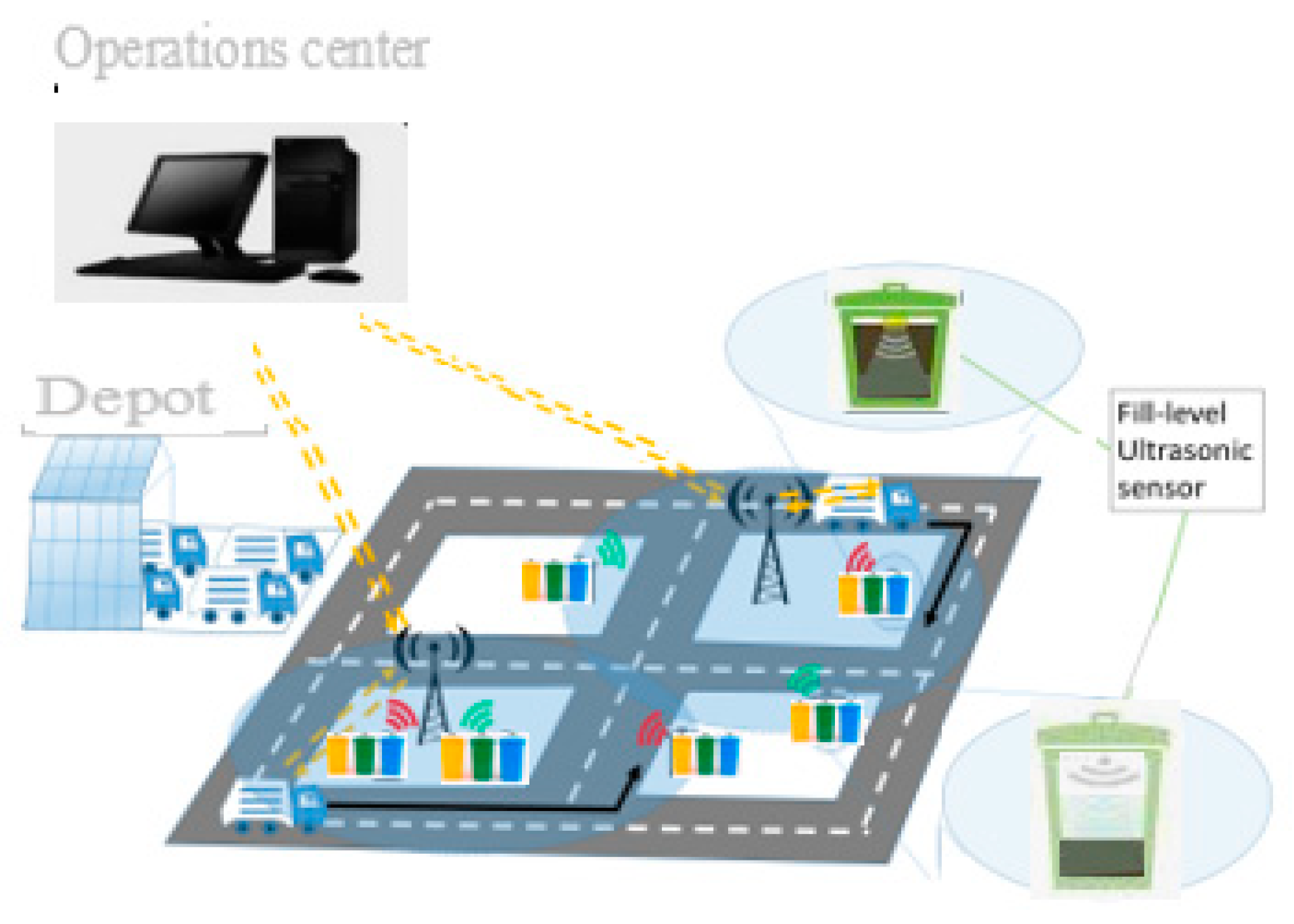
Our model proposes a separate and smart waste management problem that considers real-time information on the filling level of fragmented bins; each part is dedicated to a specific waste type to define dynamic routes for each compartmentalized vehicle. The signal base station receives information on the amount of waste in each intelligent bin at each station. It then communicates this information to the depot, which then sends compartmentalized vehicles to collect the selected separate waste stations. When a new station appears, the main task of the dispatching center is to include the new station in the current routing plan. Scheduled routes must be rescheduled depending on the position and waste load of the alarmed stations. The waste types, can be transported on the same vehicle without mixing the types; this is done by dividing the capacity of each vehicle into a number of compartments where each compartment can accommodate a waste type from one or more stations.
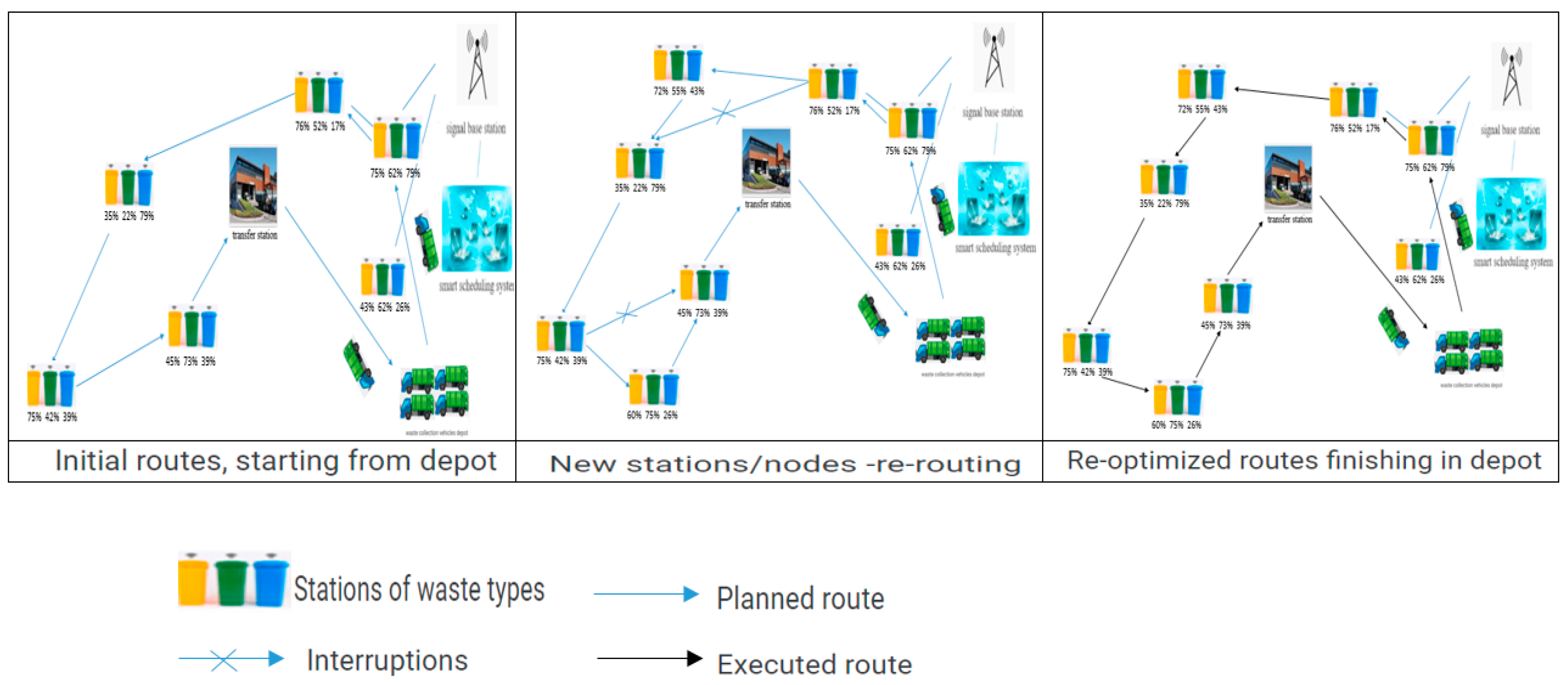
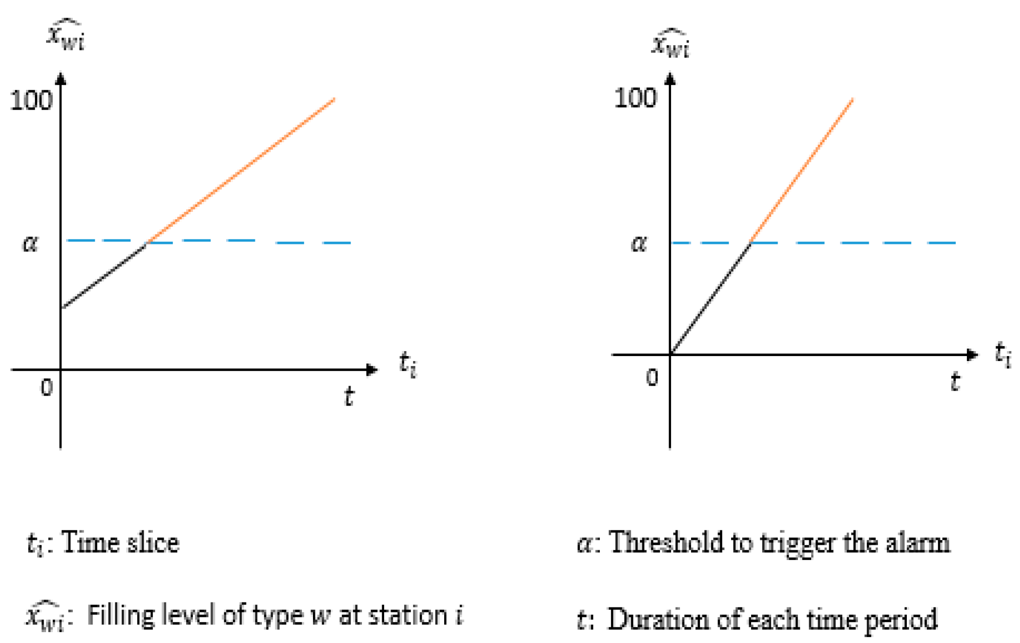
As shown in
Figure 1, the dynamic event considered is the appearance of a station that contains at least one waste type having a filling level
such as
(
is the threshold to trigger the alarm for each waste type) (
Figure 2).
Our problem can be defined as follows: given a set of n stations (each station contains bins, and each bin is designated for a specific type of waste), a group of homogeneous compartmentalized vehicles, a transfer station where vehicles unload different types of waste collected in the bins, and a depot (where all vehicles begin and complete their path), a complete undirected graph is defined over nodes, with distances for each edge in the graph. Each bin of type w in station has a maximum capacity . Let be the travel cost per unit of distance travelled. Each compartment in a vehicle has a capacity (in kg).
The sensors inside the bins transmit information on the bins’ fill levels in
, which is transformed into kilograms. To model and solve this problem, we will adopt the approach proposed by [
35], which consists of dividing the working day into time slices
(
Figure 3); each time slice represents a partial static Multi-Compartment Vehicle Routing Problem (M-CVRP), which optimizes the route of each vehicle, where vehicles must serve all known stations at minimum cost while satisfying the capacity of the vehicle compartments, and the bins capacity.
The discretization strategy we followed is different from that proposed in the literature because we have stations that can be visited more than once in the same working day. The vehicle visits the stations that triggered the alarm, and collects the alarm types first. Then it contains the other waste types in the corresponding compartments if the capacity of each case is sufficient after visiting all the stations that triggered the alarm for each waste type.
At the start of the day, the compartmentalized vehicles leave the central depot with a route plan containing the stations that were not collected the day before until the alarms are triggered to redefine the routes.
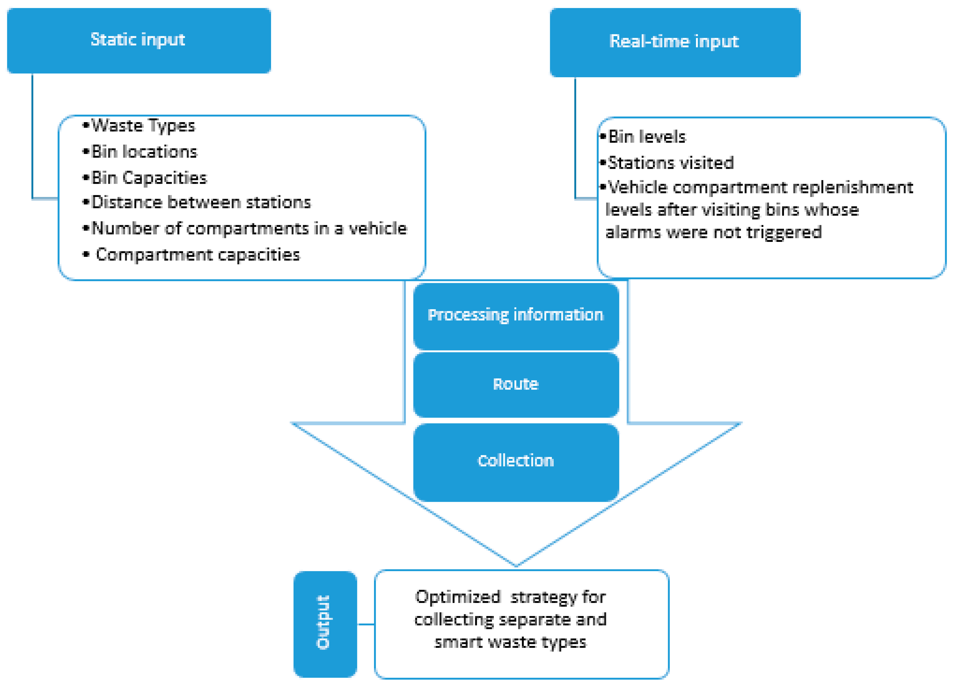
The problem of separate and intelligent waste collection is assessed here. Consider the input data, which can be divided into two main types: static and real-time inputs data (
Figure 4):
- -
The static inputs are the information on the waste types and the bin’s positions in a station, the bin’s capacity, and the distance between the stations. Secondly, concerning vehicles, the static inputs are the number of compartments, which are identified with the number of waste types and the capacity of each compartment.
- -
Real-time inputs are received by existing tracking technology devices inside the bins to give the quantity value of each container in each station, the effective replenishment of bins after each visit, and the vehicle charge after collecting each type is not alarming.
The real-time traceability system required for real-time entry is based on three main levels, namely the bins, the vehicles, and the operation center, each one connected to the other as indicated in
Figure 5.
The types of vehicles used are compartmentalized vehicles. For this, it is assumed that each compartment is dedicated to a specific waste type. The bins of each station inform the operations center of the waste type level in terms of volume, which is converted into weight, and it triggers the alarm when it reaches a predetermined maximum threshold for each type. The operations center knows the location of the bins at each station, the weight of the loaded waste, and the current weight of vehicle capacity. The operations center sends the information to the vehicle at the depot and inviting to visit the alarmed stations according to the route model proposed taking into account the ferries mentioned and at each station serviced, the vehicle communicates to the operating center the quantity of loaded waste for each type not alarmed.
4. Mathematical Modelling
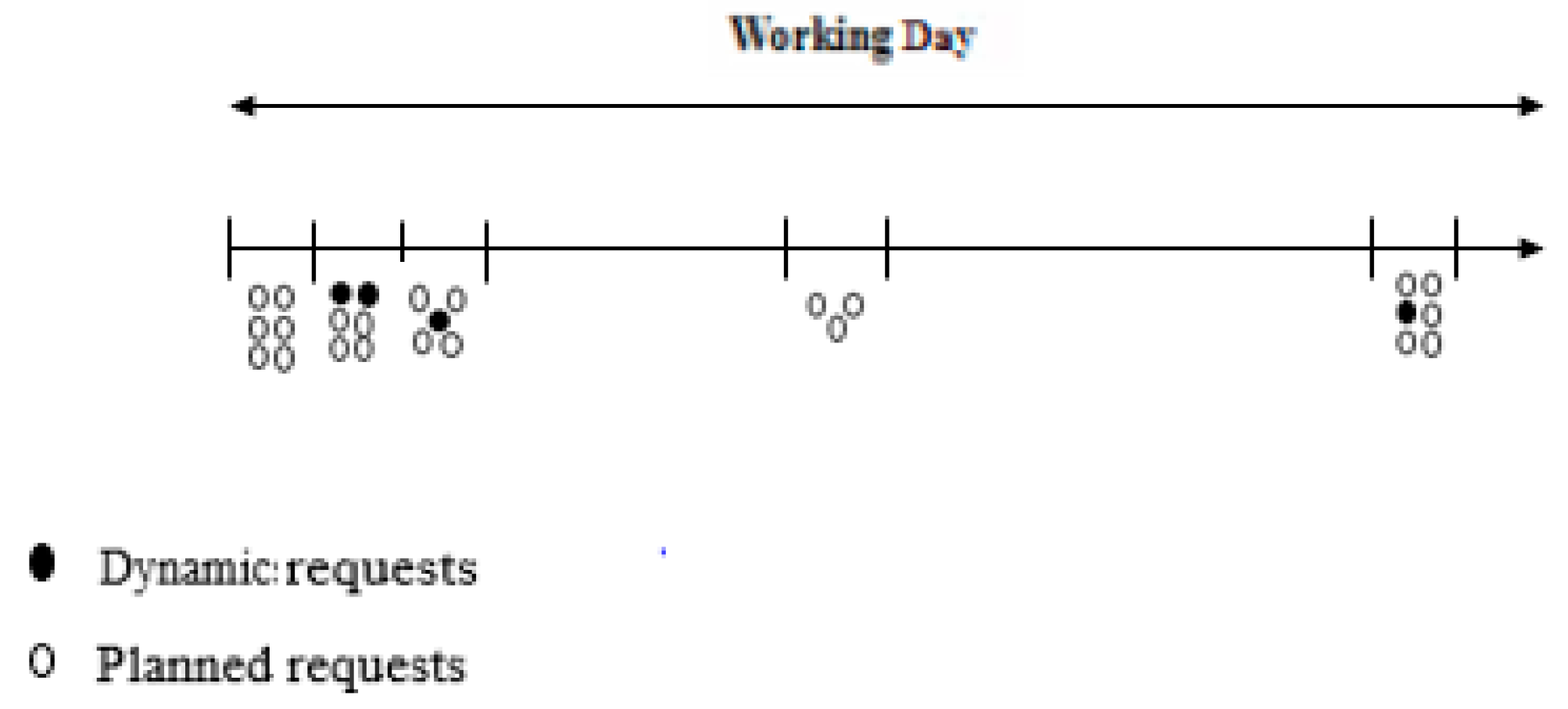
In this problem, some vehicles visit several bins during working hours. Unlike static M-CVRP, where all stations are defined at the beginning of the operation, DM-CVRP allows newly arriving stations during working hours (i.e., the stations alarmed during the time slice). When a new station comes, the dispatcher or the company must decide whether to accept or reject the service request. At each time slice, getting a new order means the station will be called in the following time slices. On the other hand, the refusal means it will be called during the work slices on the next day.
In this paper, a DM-CVRP is modeled as sequences of the time slice. Let H is the total working hours. A time slice divides the H time into several time intervals b, such that each time slice is considered a static M-CVRP
Where:
Considers the well-known stations from the previous working day; these stations are overcarried to the next working day.
: Consider the stations received during the previous time slices and some of the stations received on the last working day.
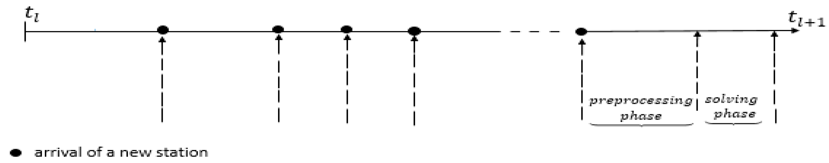
Each time slice contains a continuity period, and a decision period (see
Figure 6). The system will enter the decision period at the end of the time slice to redefine the itineraries of the following time slices, and consider the new stations that have arrived in the current time slice. The decision period can be divided into preprocessing phase and the solution phase.
The preprocessing phase is used to determine whether new requests can be added or rejected, and the solution phase is used to reschedule the routes of all vehicles in subsequent time slices. Each resolution phase will be considered all the stations already programmed in the time slices and the new stations that have arrived and can be visited.
At the end of each time slice, the vehicle’s position current is marked, and the last stations visited are considered fictitious depots in the next time slice.
A static M-CVRP is applied to obtain the optimal route based on the current information.
Figure 3 illustrates this approach.
At the beginning of the working hours, all vehicles start from the depot. Thus, the initial point of all vehicles for the time interval is {0}. For the other time intervals, , , each vehicle starts from its current position. During the time interval , , the constructed route must consider all the stations which have already been programmed and the new stations that arrived during the previous time slices which can be visited. In addition, {0} and are also taken into account since it is the last station visited before each vehicle’s destination.
Some stations may not be served, due to limited hours working. In this case, these stations will be served during the next working hours. Thus, the problem not only determines the optimal route for all stations but also selects which stations should be performed, and what waste types can be collected during the current hours of the working day.
The proposed formulation is based on the following assumptions:
The fleet is homogeneous.
Vehicles have multiple compartments.
Each vehicle starts its tour, and the end returns to the depot.
Each station is visited only once by a vehicle in a time slice. But it can be called more than once in a working day.
Each compartment is dedicated to one type of waste.
The number of compartments is equal to the number of waste types.
4.1. Index Sets
= {1…}: Set of stations (each station contains bins) and the depot 0, and the transfer station
: Set of waste types
Set of compartmentalized vehicles available (the vehicles have the same number of compartments)
: Set of compartments for each vehicle
For each station either:
: Set of the waste types that have not alarmed
: Set of the waste types that have alarmed
Note that for each station we have:
: Set containing orders known at the working day start, {1, …, b}
:The set of new stations which are triggered the alarm before the time slice and which can be visited
: Set the stations considered in the time slice
If a new station has agreed to be visited in a time slice, this station will be added to the set. Then the set of stations considered in the time slice is:, because a station may be visited more than once in the same time slice. For , the set of stations considered is: .
4.2. Parameters
: The last station served by the vehicle at the time slice
: The bin capacity of type
C: traveling cost per distance unit
: Distance between node and node
: The quantity of waste in the bin (in kg) of type in station (calculated using the information sent by the sensor in , which is converted to kg)
: The sum of the quantities alarmed at all stations for each waste type
: The capacity of compartment for each vehicle
: Penalty for bin overflow for type in station
: The maximum threshold for the waste amount in the bin
: Number of compartments for each vehicle (it is assumed that the number of waste types and the number of bins are equal in each station)
: Number of containers that have alarmed for type
4.3. Decision Variables
We define the variables of our model as follows: Level of a bin’s overflow
: The amount of waste type flowing on arc , by vehicle in kg
The static M-CVRP in each continuity period for each time slice can be formulated as the following integer program:
4.4. Model
The objective function (1) contains two parts; the first considers the cost for the total distance traveled, while the second is the cost of penalty caused by exceeding the bin capacity.
The constraints of the model are as follows:
s.t
Constraints (2)–(4) ensures that each vehicle starts at the last station that has been committed to it and returns to the transfer station to unload the collected waste. Constraints (5) express that when a vehicle arrives at station , it must exit. Constraint (6) ensures that the number of vehicles returning to the transfer station equals the number of vehicles returning to the depot. Constraints (7) ensure that each waste type at station is assigned to precisely one vehicle; a separate collection of a single waste type does not exist. Constraint (8) warrants that if the vehicle visits the station, it must precisely collect at least one waste type. Constraint (9) ensures that the number of waste types does not exceed the maximum number of compartments. Constraint (10) warrants that for each case of vehicle , its capacity is not exceeded by the sum of the quantities collected. Constraint (11) states that if a bin in station is selected, it must be visited by a vehicle . Constraint (12) guarantees that a station is visited when the fill-level of at least one bin of type achieves a predetermined threshold. Constraints (13) to (15) guarantee that each alarmed waste type is collected, and can also collect non-alarmed types if the capacity is sufficient after visiting all the stations that triggered the alarm. Constraint (16) means that vehicles are empty at the transfer station before heading to the depot. The overflow constraint (17) ensures that any overflow is considered. Constraints in equations (18) to (23) are domains for the variables.
5. Methods and Results
5.1. Model Validation
In this section, we study the validation of our mathematical model. Validating the model with data and constraints makes it possible to verify the operation of the constraints. Once a solution is found, the formulation checks whose constraints have been modeled so they can be alerted in case of error.
5.1.1. Transport Network Data
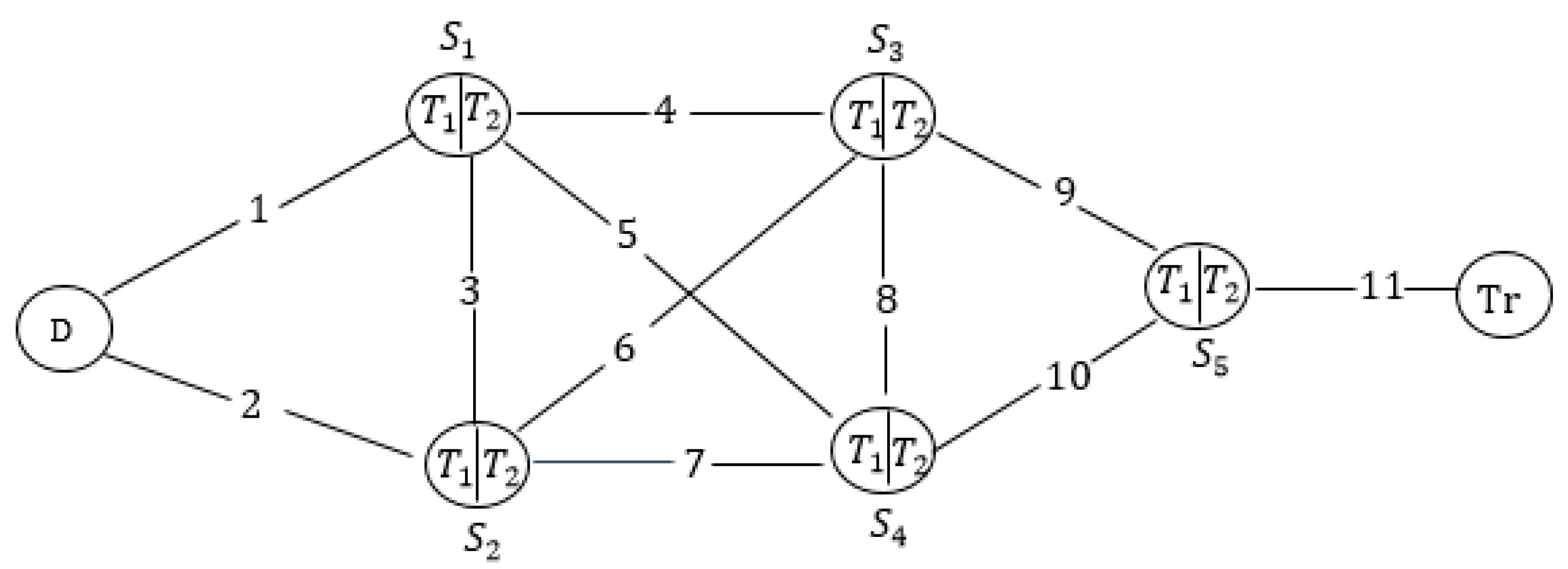
To solve the problem by the CPLEX optimizer, we test our model with small examples. For this, we are dealing with an example composed of 5 stations, each station contains two waste types, 11 arcs, and 10 lines between the depot and the transfer station. Since our objective is to validate our mathematical model, we fixed the arc length in all arcs to 1000 m, the network shown in
Figure 7.
In this example, we studied nine paths between the depot and transfer station. The paths are as follows:
Path1: D-1-3-5-Tr
Path2: D-1-3-4-5-Tr
Path3: D-1-2-3-4-5-Tr
Path4: D-1-2-4-5-Tr
Path5: D-1-4-5-Tr
Path6: D-1-2-4-3-5-Tr
Path7: D-2-3-5-Tr
Path8: D-2-3-4-5-Tr
Path9: D-2-4-5-Tr
In this subsection, our objective is to validate our mathematical model therefore, we assumed that the number of lines limited in nine even there are other lines to add. The purpose is to simplify the validation of the model without changing the real problem.
Table 1 collect the data values. The objective is to find an optimal waste collection that allows each vehicle to go from the depot to the transfer station and return to the depot. To test our model on this example we give different values to the amount of waste in the bin (in kg) of each type in each station
5.1.2. Results
The problem is solved for each of the objectives, because CPLEX can only solve nonobjective problems. The first objective is the cost for the total distance traveled, while the second is the cost of penalty caused by exceeding the bin capacity.
We can see in
Table 2 that the number of stations visited is equal to the number of stations existing in each line because it is assumed that the stations have at least one bin with a filling level greater than or equal to 70% of the bin capacity. The vehicles can collect the bins with a filling level lower than 70% if the corresponding compartment capacity is sufficient after having visited all the stations triggering the alarm. Otherwise, the vehicle cannot collect the type in the corresponding compartment. As in lines 3 and 6, we can see that the vehicle at a station has collected type 1 but not collected type 2. Moreover, all the bins are visited before overflowing.
5.2. Genetic Algorithm for Solving the DM-CVRP
DM-CVRP is an NP-hard problem; exact-solving methods have become very time-consuming. So we have selected the genetic algorithm as an optimization tool in this article. The choice is mainly due to its simplicity, use ease, and efficiency in high-complexity problems. In this section, we adapt the genetic algorithm for each static M-CVRP at each time slice to solve the DM-CVRP.
Our system designed to solve DM-CVRP is composed of two central systems:
- -
The first preprocessing phase is responsible for receiving and adding new stations and divides the working day into a predefined number of time slices. Each slice represents a static VRP. This system manages all the entrances and exits and organizes the GA.
- -
The second solving phase, which contains the route optimization process and solutions, executes the GA to solve the static VRP in each time slice generated by the preprocessing step. To this end, a hybrid GA was proposed to find the best solution for each given time slice until the stopping condition.
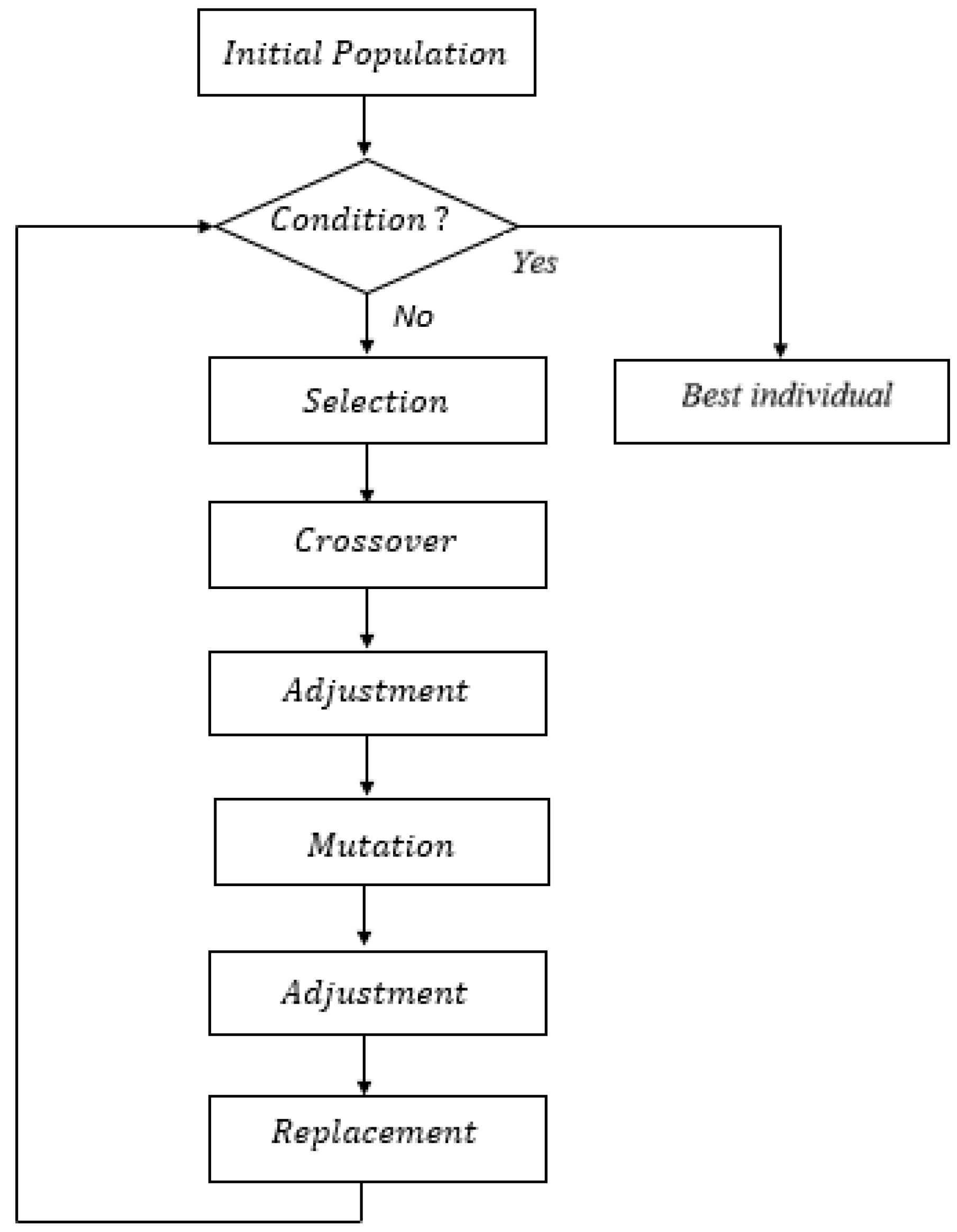
John Holland developed a Genetic Algorithm in 1975. The algorithm’s idea is to translate the problem into a genetic representation or a chromosome, which is used to define a solution. Each solution is associated with a numerical value called fitness according to the function of this solution. At each iteration, a certain number of solutions are selected according to their fitness to create new ones by applying genetic operators (crossover and mutation). At the end of the iteration, a replacement step is applied to select the solutions for the next generation. We use GA in this paper, and we hybrid it by heuristic methods.
The general structure of the Genetic Algorithm is as follows:
Until the condition stops.
Our hybrid genetic algorithm is shown in
Figure 8.
5.2.1. Preprocessing Phase
The preprocessing phase manages the new stations, creates static problems, and engages the stations on compartmentalized vehicles. It is a stage between the arrival of new stations and the optimization phase. The first static problem created for the first time consists of all remaining stations from the previous business day. The following static problems consider stations received during the last time slices. In these problems, the compartmentalized vehicle departs from whatever committed station it has just visited with appropriate capacity changes. After each time slice, the best solution is chosen. When a vehicle has used all its capacity, it is sent back to the depot.
5.2.2. Solving Phase
A GA strategy is executed for each static VRP created as described above. Each chromosome in a population represents a possible solution to a static VRP.
Encoding the Solutions
For each time slice , each solution is composed of routes for vehicles and collection bins. The following table represents the solution for a vehicle .
In the example illustrated in
Table 3. Route 1 is served by vehicle 1, which visits the ordered list from station 2, starting with
(
is the last station operated by vehicle
at time slice
), until the last station 1 before visiting the transfer station to unload the collected quantities, and then returns to the depot. Vehicle 1 collects types 1 and 3 in station 2; it collects types 2, 3, and 4 at station 5, and it collects types 1 and 4 at station 1.
Initial Population
A routing solution based on a list of integer numbers, where 1 to represent stations, represents the transfer station, and 0 represents the depot. The heuristic constructs the routing of available vehicles beginning with the first one by inserting the request’s origin and destination in its trajectory to find a suitable solution for DM-CVRP. If the compartment capacity of the vehicle is reached, we move on to the second vehicle, up to all the stations that have been served. This heuristic is divided into two steps, the first step is for the first time slice, and the second step is for the other time slices:
- ▪
The initial population of the first time slice:
The working day begins with the first time slice that indicates that depot 0 is inserted, and every time, if a station respects the capacity constraint must be inserted in the route (remaining vehicle capacities for the types triggering the alarm) until all the stations in the list have been affected. If the vehicle compartment capacity is reached for all waste types, the vehicle visits the transfer station and then returns to the depot. If the vehicle capacity constraint is not respected for any remaining station in the list, the current vehicle will move to the transfer station, then to the depot. The algorithm marks the last station visited, and this station is considered a depot for the next time slice . This heuristic is based on the following algorithm:
| Algorithm 1: Creation of the initial population. |
Select randomly a stationfrom the list
Foreach waste typeI in the station
If there is wI such that the quantityis less than or equal to the capacity remaining
in compartment m (With m being the corresponding compartment to the type
w in the vehicle v)
Collects the type w in the corresponding compartment and decreases the capacity of the
compartment m of the vehicle v (← )
End for
End If
For each waste type J in the station
If there exists w J such that the quantity is less than or equal to the capacity
remaining in the compartment m of the vehicles after visiting all the stations triggering
the alarm for the type w
Collects the type win the corresponding compartment and decrease capacity of the
compartment m of the vehicle v (←
End for
End If
If all types trigger the alarm in the station have been transported
Remove this station from the list
Else
Update in list
Else
Get back to 3
End If
End While
If the vehicle capacity is reached for all types
The vehicle v visits the transfer station, and returns to the depot
v = v + 1
Get back to 3
Else
Get back to 3
End If
- 4.
Returns the last visited station ( is the last station visited in time slice )
|
- ▪
The initial population of the other time slices:
The second step of the heuristic create the initial solutions for the time intervals . The same process as the first step is used to generate the initial solutions in the time slices , except that the list of stations considers already programmed stations in the current time slice and the new stations triggering the alarm in the previous time slice. A station can be visited more than once in the same working day because each time a type in a station triggers the alarm, this station will enter the list of stations to be visited in the next time slice. Therefore, the list of stations considered in the time such that is .
At each time slice, the depot considered is the last station visited in the previous time slice.
Selection
Computed fitness allows the selection of members for the next generation; this can be done using different selection types, like Roulette, Tournament, and Random.
The tournament selection is adopted to choose some chromosomes to undergo genetic operations. The most common tournament method is the binary tournament, where we select two individuals randomly in the population. We choose the best one (which has the smallest fitness value). This process is repeated until the obtained required number of individuals is reached. On the other hand, after applying genetic operators, selection for replacement determines which individuals will disappear from the population in each generation and which strong individuals survive in the next generation population.
For each individual, we associate a fitness function that corresponds to a compromise between the two objectives, namely the total distance traveled cost and the cost of the penalty caused by exceeding the bin capacity. We represent this function as follows:
where
and
represent the importance of the two objectives considered.
Crossover Procedure
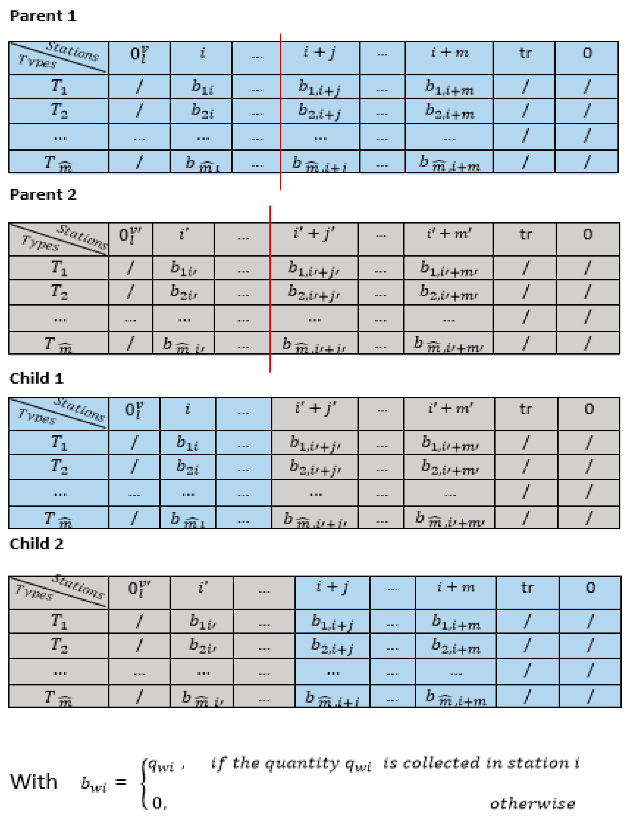
Crossover is a genetic operator that combines two chromosomes called “parents” to produce a new solution called “child”. The purpose of using crossover is that the new solution can be better than both parents can if it takes the best characteristics from each parent.
Two parents’ p1 and p2, are selected from the population. The proposed crossover takes place in two phases:
- -
The first phase randomly chooses a crossing point k for each arc (the red line in
Figure 9 and
Figure 10). The crossover procedure used in this paper is eluted as follows: the first part of the first parent is copied as the first part of child 1, and then the elements of the second part of this parent are considered the second part of child 2. The first part of the second parent is copied as the first part of child 2, and then the elements of the second part of this parent are considered the second part of child 1. The two parts for each child are combined to form a new path (See
Figure 9).
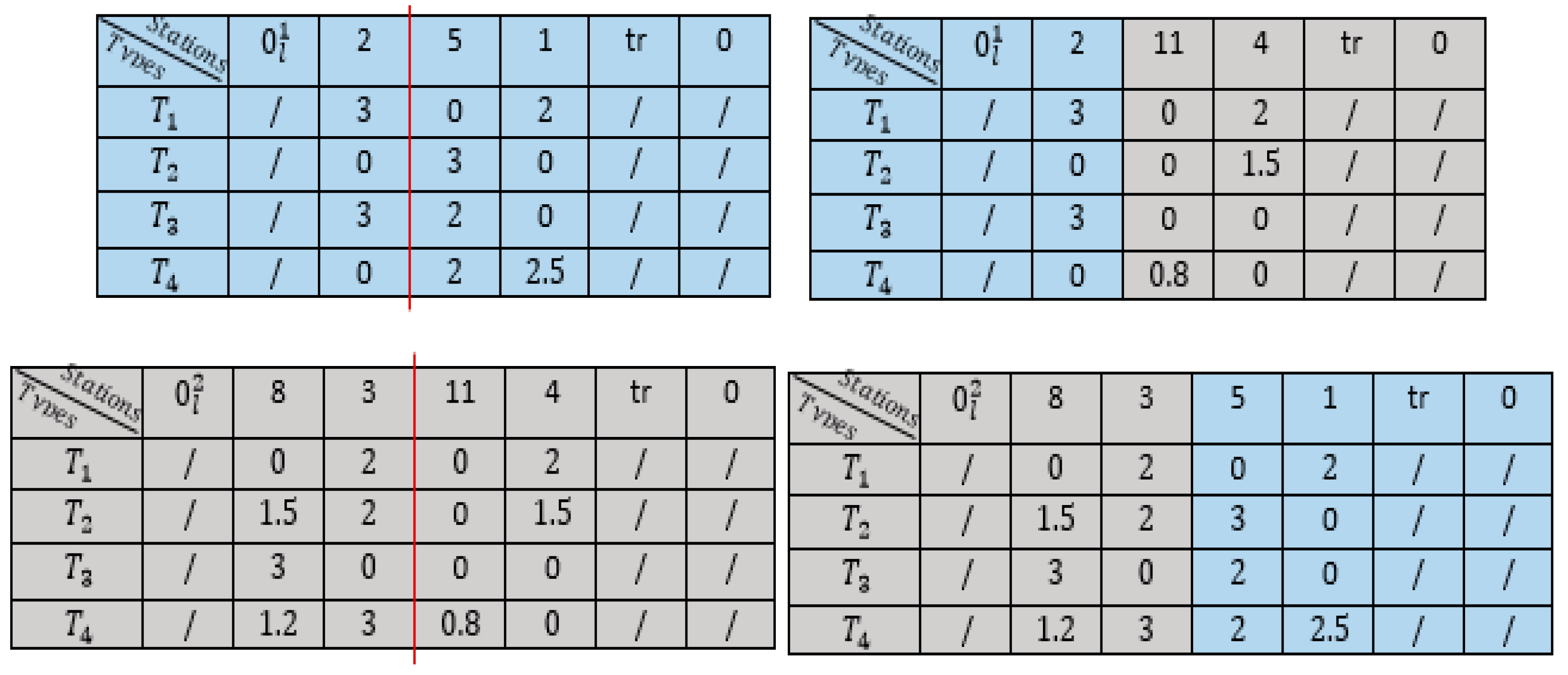
- -
After crossing, the result does not always correspond to a feasible solution. We illustrate this situation with the example in
Figure 10.
We assume that we have four types of waste and that the trucks have four compartments.
We assume that each truck has a capacity of 23 tons distributed as follows: The first compartment capacity is 7 tons, the second compartment capacity is 5 tons, the third compartment capacity is 6 tons, and the fourth compartment capacity is 5 tons.
Note that the obtained result does not present a feasible solution (see
Figure 10), for child 2, the sum of the quantities transported in compartments 2 and 4 is more significant than the capacities of the corresponding compartment. Therefore, we have to make some adjustments, so the second phase is testing the feasibility of these new chromosomes using the heuristic illustrated in the following algorithm for child 1 (the same algorithm is applied to modify child 2):
| Algorithm 2: Modification of the crossover operator. |
Foreach vehicle
For each stationin the path of child 1
For each waste typein the station
While
If ()
Collected all waste type (if in the corresponding compartment of vehicle
for child
Else
Repeat
For (j=… )
Calculate
If
Replace by 0 for child 1
Else
Collected the waste type in the station in the corresponding compartment of
vehicle for child , and calculate +
get back to 11
End If
End For
End If
While
End While
p = p + 1
End While
End For
End For
End For |
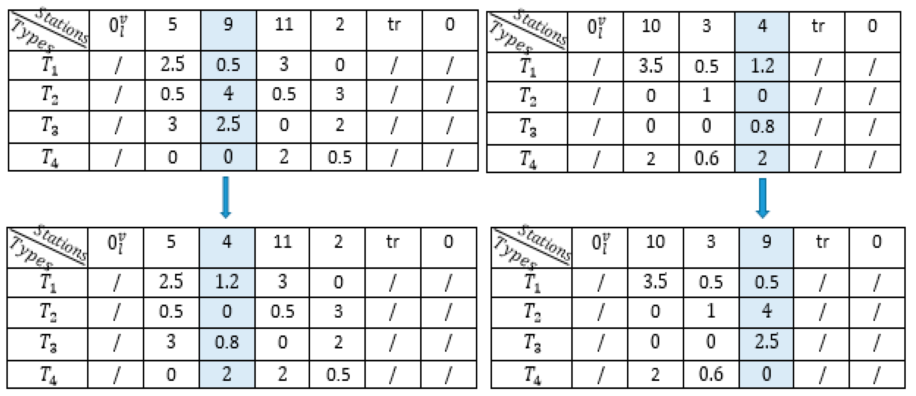
Mutation Procedure
The mutation is applied with a certain probability. The mutation operator allows modifying an individual’s genes to find other parts that are very different. At this point, some parents are chosen from the population to apply the mutation operation. We use the inversion operator, which is simple in that it generates a point along the length of two chromosome genes and then inverts those two points (two stations). An example of inversion is shown in
Figure 11.
After the mutation, the sum of the quantities collected for the type at the stations visited may be greater than the corresponding compartment capacity.
To keep the feasibility of the solution, we propose the following modification algorithm:
| Algorithm 3: Modification of the mutation operator. |
(p is the change point)
If
Else
Collected the waste type in the station in the corresponding compartment of vehicle
get back to 3
End If
End For
End |
Before studying the example based on the real data of valorsul using our hybrid genetic algorithm (HGA), we treat the example presented in
Section 5.1 to show the efficiency of the approach used HGA.
Table 4 shows the results found by applying HGA method and the results that we found using the CPLEX software (exact method). To illustrate our results, we calculate the quantity collected for each type in each arc (TCW1 & TCW2), the number of visited bins for each type at each station (TVB1 & TVB2), and the bins overflow level in each arc, and the transport cost (TC). We obtained the results shown in
Table 4.
In
Table 4, we can see that the results obtained are the same for both methods (CPLEX and HGA). This happens because if the vehicle collects a waste type in a station, it collects all the quantity existing in the bin.
6. Experimental Study
6.1. Real-World Study
The case study presented in this article is based on data from those Ramos et al. [
10] and Silva, R. F. R [
29], with some modifications to adapt this data to our problem. These are the waste collection operations by Valorsul–Valorizaç˜ao e Tratamento de Resíduos S’olidos, S.A. This company operates in the region of Lisbon, the capital of Portugal. Valorsul is responsible for collecting different types of waste, including recyclable waste (glass, paper/cardboard, and plastic/metal). The collection of recyclable materials is carried out in 14 municipalities by a homogeneous fleet of vehicles based on a single depot. During compilation, the team records the fill level of the bins. It classifies them as empty (0%), less than half (25%), half (50%), more than half (75%), or full (100%). The collection system proposed by Valorsul for the collection of recyclable waste then estimates the filling level of the bins and decides whether to include these bins in the route. This estimate is calculated as follows: after having visited all the assigned collection points, the truck returns with information on the filling levels of the bins. This information and the density values provided by Valorsul from Paper and/Cardboard (PC), Plastic and/Metal (PM), and Glass (G) and the density values provided by Valorsul from PC, PM, and G (
= 40 kg/m
3;
= 20 kg/m
3;
= 300 kg/m
3; see densities in
Table 5) were used to calculate the amount collected per bin. The formula to calculate the quantity ordered per station and per type of waste follows (1.1a), where
is the quantity collected at station
of type
,
is the type density
,
is the total capacity of all bins of waste type
in station
, and
the average fill level of all containers of type
w in station
i.
For more clarification, part of the visit sequence carried out is shown in
Table 6, along with information on the filling level of each bin collected.
For example, the vehicle collected 50 kg of PC in bin 2293 (marked in red in
Table 6), calculated in Formula (1.1b).
The estimated fill level of each bin heard by Valorsul is calculated by dividing the total fill levels recorded for each bin by the number of days in the period multiplied by the time interval between routes (Ramos et al. [
10] and Silva [
29]). This estimation allows a comparison between the current situation of Valorsul and the results obtained when applying our approach.
Ramos et al. selected three routes to collect the type (paper/cardboard) to analyze the current situation (blind collection) and the future situation (installation of sensors to obtain real-time information on the filling levels of the bins). Route 6 with 68 containers, route 11 with 74 containers, and route 13 with 84 containers, totaling of 226 containers. The scalar data of the study are those presented in
Table 7.
is the cost of travel per distance unit, including fuel consumption, vehicle maintenance, and the salary of the collection team.
is the amount of waste at bin
, (considering the density of paper/cardboard), simulates the values the sensors will read and transmit daily. To apply the resolution method, we use the bin’s fill levels registered by the collection team after visiting these bins plus an expected accumulation rate per bin
. This accumulation rate was calculated by dividing the bin fill levels recorded by the collection team by the number of days that passed after the previous day the bins were collected (Ramos et al. [
10]).
For Valorsul, the types of waste are not always in the same station; there are other routes to collect plastic/metal and glass. To apply our model and our proposed approach, we assume that each station contains two bins (one for paper/cardboard, one for Metal/Plastic), and we use a two- compartment vehicle.
Table 6 shows the data from Valorsul, and we add some more data for it to be applied to our problem (from the data illustrated by Silva [
29]).
Ramos et al. considered a planning period of 30 days to collect the paper/cardboard; the profit obtained by the Valorsul for the three routes is presented in
Table 8. During the planning period, routes 6 and 11 were twice repeated, route 13 four times, and 620 bins were visited, with 12% empty and 1% overflowing. In these eight routes, the waste collected amounted to 17,000 kg, and 1200 km were traveled, resulting in an average of around 15 kg per km traveled), and the vehicle utilization rate varied between 46% and 67%.
Since we do not have data in the literature on the collection of Plastic/Metal, we will propose data presented in
Table 9. On these eight routes, it is assumed that the waste collected (Plastic/Metal) amounted to 9000 kg and the rate of use of the vehicles varied between 55% and 71.5%.
6.2. Study Results
The modified genetic algorithm applied to our model was implemented in C++ language on a Windows 10 Professional Intel(R) Xeon(R)W2155 CPU (20 CPUs) at 3.3 GHz, with 32.768 GB of RAM to test the quality and performance of the modified genetic algorithm and the proposed model.
The choice of parameters influences the results. For that, several tests were carried out on the parameters of the method (crossing and mutation) to identify the best parameters to use. We launched our program with different sizes of populations {20, 50,100,500}, and we found the best solutions for a population of size 50 individuals. Therefore, the parameters of the proposed approach are set as follows:
Crossover rate: 50% of the population size
Mutation rate: 20% of the population size
Population size: 50 individual
Number of iterations: 100 iterations
6.2.1. Experimental Results: Static M-CVRP
Our approach in the static case was tested, considering the same data presented in
Table 6, except for the amount of waste and gives in real-time. The types selected to collect with multi-compartment vehicles are Paper and/Cardboard, Plastic, and/Metal. Therefore, each vehicle needs to have two compartments, one for each type, and we consider the capacity of the two compartments given by Silva et al. 2016. In addition, we add a penalty of 1 € per kg for each bin that overflows. The value of the minimum fill level at which the containers must be visited when applying the proposed Metaheuristic is assumed to be equal to 70% of the container volume, i.e., each bin that has 70% or more of its capacity for both waste types.
After applying our approach, we can see in
Table 10 that the number of visited stations is lower than the number of visited bins given by Valorsul (233 against 620). Since the stations visited are the stations that have at least one container with a fill level greater than or equal to 70% of the bin capacity (having a bin capacity of 52.5 kg at most). We also note that there are plastic/metal type bins were collected even if their fill level did not reach the required weight. This is due to the ability of the plastic/metal type compartment to collect this waste type at each station visited after calculating the total disturbing quantities of this type.
The 73 empty bins were visited during the period in the real case, while in our approach, there are no open visited stations. Moreover, no container exceeds its maximum capacity, i.e., all bins are visited before overflowing, while there are four overflowing bins for actual Valorsul operations.
Regarding the distances, a reduction of 55.77% of the traveled distance (532 km vs. 1203 km), so we see that the total distance to be crossed in the actual case of Valorsul is twice as large. This is justified by the fact that the vehicles travel long distances to collect fewer bins, which requires a model capable of choosing the containers worth visiting according to their fill levels and location.
When the hybrid metaheuristic is applied, the vehicle usage rates are always higher than 50%, varying between 53% (day 22) and 82% (day 15). Valorsul vehicle usage rates are lower, starting at 46% (day 22) and reaching 67% (day 15) at maximum, so this allows us to say that our approach gives satisfactory results.
6.2.2. Experimental Results: Dynamic M-CVRP
In this part, we present the results of our proposed approach for the resolution of the dynamic M-CVRP, where we must satisfy the integration of new stations when the alarms are triggered for at least one waste type, then the routes have been planned. Their exploitation started by adding the characteristics below to obtain the dynamic problem:
The discretization of a working day.
The time of appearance of a station.
Our tests were carried out over six days, and we kept the parameter values used in the static case, and we simulated the length of a day by 22,000 s ( = 22,000 s), and thus the algorithm is stopped if the elapsed time is greater than or equal to . This duration is divided into time slices having variable sizes according to the course of an iteration of our approach .
This group contains six days with 5 degrees of dynamism (dod) (Messaoud et al. [
16]) which are 90%, 10%, 50%, 70%, and 30% (dod = 0% present the static case).
Table 11 reports the obtained results on the different degrees of dynamism for our modified genetic algorithm. It indicates the total traveled distance and the number of stations visited. We note, on the one hand, that respecting all the constraints, the dynamic aspect influences the number of stations visited and the distances covered, it is easy to see, on the one hand, that if we increase the degree of dynamism, the total distance increases, then it decreases when the degree reaches 50%, then it goes up or remains unstable, and on the other hand, we notice that in some cases, even if the distance increases, the number of stations visited remains the same, or else diminished, This is due to the fact that the number of visited stations does not depend only on the distance traveled but specifically on the number of stations triggering the alarm, and which are integrated into the different time slices. And in DVRP, the vehicle can service stations on its way, which can reduce the distances covered.
In static VRP, the more contains more stations, the simulation results tend to be much better because the vehicle often returns to the depot with approximately full loading, and thus, the vehicle number is reduced. However, in DVRP, it is uncertain that the optimization result is better when contains more stations because there are undefined factors.
Generally, at the end of each day, the number of unvisited stations with at least one waste type with a filling rate greater than or equal to 70% is negligible compared to the number of stations having triggered the alarm and which is visited regardless of the dynamism degree. This makes it possible to say that our approach gives satisfactory results in terms of quality of service in the dynamic case.
The approaches proposed by existing works in the literature for the smart waste collection problem did not respect all the constraints, especially in the dynamic case; this is why our results in the dynamic case, were not compared with those found in the literature. In addition, to show the effectiveness of our approach, we focused on comparing our result in the static case with the current situation of the Valorsul Company.
7. Conclusions
This work introduces the problem of separate waste collection in smart cities, where it is assumed that each station contains a limited number of bins; each bin is specialized for a single type of waste. The uncertainty is considered regarding the amount of waste in each container at each station by installing sensors capable of real-time reading and transmitting the stations’ fill levels. This makes it possible to consider the problem as a multi-compartment vehicle routing problem to collect only the stations having at least one more attractive bin, which improves the efficiency of operations. For that, we proposed a mathematical model whose objective is to minimize total transport costs, including crossed distance and penalties caused by bin overflowing. To validate our model we tested the model using the CPLEX Optimizer on a small example, since the problem was a very complicated one.
We have proposed a static M-CVRP resolution approach based on genetic algorithm hybridization. Afterward, we adapted this approach to solve the M-CVRP in the dynamic case; in the latter, during the execution of the planned route, we integrated new stations triggering the alarm for at least one waste type.
To validate our approaches, we used a real dataset from Valorsul with some modifications to adapt these data to our problem, where we dedicated to the collection of two types of recyclable waste Paper/Cardboard (PC) and Plastic/Metal (PM) using multi-compartment vehicles. We were able to ensure the effectiveness of our approach based on the results of the static case, which are very encouraging. Moreover, in the dynamic case, we used the definition of the degree of dynamism with such significant results established.


