Modeling and Analyzing a Multi-Objective Financial Planning Model Using Goal Programming

Abstract

Optimal financial planning plays a vital role in maintaining concentration and on the path as the organization extends, when new challenges materialize, and when unpredictable situations pounded. This study aims to develop and implement a goal programming model to evaluate financial planning based on the annual financial report of Saudi Basic Industries Corporation (SABIC), which assisted it in developing the financial planning model. This study is mainly designed to analyze SABIC’s budgeting structure; therefore, in order to maximize the benefits from the whole budget, goal programming is implemented for the entire budget. As a result of this study, we identified the following objectives as specific: reduced expenses, increased revenue, increased net profit, increased fixed assets, reduced debt, and increased equity share participation as a result of this project. Moreover, the analysis involved determining whether all objectives were met at the end of the study. Consequently, this study will benefit industrial institutions in achieving their financial objectives.

1. Introduction

Developing a financial plan is an essential component of the success of any industry. A good understanding of finance is critical for industrialists to take their businesses to new heights and survive more challenging economic conditions. In the realm of the statements mentioned above, this study illustrates an industry’s multi-objective decision-making problem. The multi-objective decision-making problem can be encountered in many applications, such as solid waste; accounting; finance; marketing; quality control; human resources; production; transportation; site selection; space studies; agriculture; telecommunication; etc. One method that can be applied to the problem of multi-objective financial planning is goal programming because it is a powerful technique for solving multi-objective decision-making problems, one of the most challenging problems. Several fields have benefited from goal programming in recent years due to its ability to generate significant results.

Undoubtedly, financial planning is one of the most critical components of any business. By considering these facts, it was decided that this study would focus on evaluating SABIC’s financial planning. Financial analysis is necessary to develop strategies for determining financial strength and identifying potential enhancements to the industry. In addition, this study aims to evaluate the company’s financial plan to maximize income and minimize costs as much as possible. As a result of the study, the following specific goals will be achieved: evaluate the maximized assets, assess the minimized total liabilities, assess maximized equity, maximized gross profit evaluation, and evaluate the maximum operating [1,2].

In addition to production planning, scheduling, tourism management, banking financial management, and financial institutions, goal programming techniques are now used in various fields. Ekezie and Onuoha studied goal programming for budget allocation in institutions and developed a model for analyzing the institute’s budgeting system. In addition, they emphasized that the institution should continue to use its budget allocation formula with scientific methods [3]. F. A. Farahata and M. El Sayed proposed a goal programming model with two types of uncertainty. There are two approximation models: an upper approximation model and a lower approximation model. A lexicographical goal programming method has also been suggested for solving these upper and lower approximation models [4]. Boppana and Jannes developed a multi-objective goal programming (MOGP) model for a real-world manufacturing situation to show the trade-off between the goals of the customer, the product, and the manufacturing process. The study’s results revealed that a planning tool could be valuable in making decisions [5].

Thomas and Daniel examined financial management decision situations using goal programming and summarized its limitations [6]. According to James E. Hotvedt, linear programming to solve multi-objective problems requires that all incommensurable goals be transformed into a standard unit of measure to solve the problem [7]. Mehrdad Tamiz et al. concluded that goal programming could be used as a pragmatic and flexible approach to solving complex decision problems involving many objectives, variables, and constraints [8]. With the help of a goal programming model, Weng Siew et al. determined several financial parameters for shipping companies. In order to enhance the developed model, the most suitable values for all goals are used as target values to enable a better comparison of achievement levels [9]. According to Carlos Romero, it is critical to establish a bridge between the different MCDM approaches to achieve mutual benefits [10]. In a study by Kruger et al., it was suggested that specific strategic goals include returns, risks, liquidity, capital adequacy, and growth in market share. Because these goals conflict, a simple linear programming approach will not suffice, and one must resort to a multi-objective strategy such as goal programming [11]. A study by Luis Diaz-Balteiroa and Carlos Romero concluded that goal programming techniques efficiently integrate all the criteria into a mathematical program that could be used to solve real-life problems [12]. Furthermore, Jamalnia and Soukhakian developed aggregate production planning in a fuzzy environment and concluded that fuzzy sets theory could be used in goal programming to specify imprecise aspiration levels [13].

A model was developed by Chen et al. to optimize the financial management of a Malaysian Public Bank. This study found that the model was capable of achieving all goals [14]. For the optimization of multiple criteria problems, James S. Dyer used a goal programming algorithm that requires communication between the relevant decision-maker and the algorithm [15]. Alan used individual goals as a practical and valuable tool without a priority coefficient. This tool provided the financial planner with a powerful ‘what-if’ device to evaluate the various trade-offs among the conflicting goals and arrive at a satisfactory solution [16].

In order to solve the personal financial planning problem more effectively than traditional approaches, Chieh-Yow proposed a generalized unique financial planning programming model with multiple fuzzy goals [17]. The goal programming model used by Shafer and Rogers to form manufacturing cells identified that a minimum setup time, a minimum intercellular movement, a minimum investment in new equipment, and maintaining acceptable utilization levels were the multiple objectives they identified [18]. According to Ajibola et al., UBA’s financial statement management was analyzed using a model developed based on goal programming. As a result, they concluded that the bank should convert its liabilities into earning assets as soon as possible [19]. Romero and Rehman have noted that both lexicographic goal programming, as well as weighted goal programming are widely used as goal programming variants [20]. Further, Marc J. Schniederjans et al. stated that Goal Programming is used as a model that utilizes the analytic hierarchy process to evaluate property attributes before making an optimal house selection decision [21]. Eventually, by using a pre-emptive fuzzy goal programming approach, Hossein Mirzaei et al. demonstrated that a mixed-integer linear programming model could mathematically formulate problems that can then be automated using a fuzzy goal programming approach [22].

Lam et al. used a goal programming approach to optimize the financial management of various electronic companies according to their financial parameters and the optimum management item. As a result, they found that goal programming produces the best possible solutions for each organization [23]. A multi-objective integer linear programming model based on the Markov chain method is proposed by Devendra Choudhary and Ravi Shankar for the joint decision-making of the lot-sizing problem, the supplier selection problem, and the carrier selection problem [24]. It was concluded by Marc J. Schniederjans and Rick L. Wilson’s analytic that the combination of the analytical hierarchy process and goal programming methodologies helped overcome some weaknesses observed when either method is used independently [25]. Lakshmi et al. proposed financial planning to acquire incommensurable and conflicting plans using goal programming, and they concentrated on maximizing both the capital system and gain in returns [26]. Schniederjans, Marc J. et al. proposed, in their paper, a goal programming model incorporating elements of critical path method and concurrent engineering to enhance the planning of value analysis projects [27]. A study by Ali AlArjani and Teg Alam indicates that lexicographic goal programming has become one of the most popular approaches to multi-objective criteria. They developed a lexicographic goal programming model to analyze and optimize the performance management of Al Rajhi Bank, a Saudi Arabian bank, and they found that based on the optimal solution, Al Rajhi Bank can accomplish all its objectives [28]. In addition, by using multi-objective optimization, Flavia and Anisor integrated organizational performance’s three primary objectives: selling more, minimizing expenses, and increasing productivity. Hence, they analyzed whether the presented system delivers something that no framework does by combining objective and subjective methods [29]. Belaid et al. delivered a comprehensive literature study of the GP application within the accounting field. They suggested a model that acts as an approach for accountants to determine the most suitable variant of GP to deal with specific accounting-related decision-making situations [30].

A model for SABIC’s optimal financial management is proposed in this study.

2. Materials and Methods

2.1. Goal Programming Problem (GPP)

Several industrial problems have been solved in the last fifty years using Goal Programming techniques and Goal Programming models. The goal programming approach resolves multi-objective optimization problems by balancing conflicting objectives. In this process, the most effective indicator of goal achievement is determined. By using the goal-programming model, multiple and often incompatible goals can be accommodated.

2.2. Nomenclature

The following nomenclature is used in the development of the model, as shown in

Table 1. Modeling notations.

Notation	Description
m	Number of goals
p	Constraints of the system
n	Number of decision variables
Z	Objective function (Summation of all deviations)
$a_{ij}$	Coefficient associated with variable j in the ith goal
$x_j$	Variable that represents the jth decision
bi	Value associated with the right-hand side
$d_i^{-}$	Negative deviation from the ith goal (underachievement)
$d_i^{+}$	Positive deviation from the target (overachievement)
$p_i$	Preemptive importance factors of the ith goal.
$w_i^{+}$	Non-negative constants that represent relative weights for positive deviations
$w_i^{-}$	Non-negative constants that represent relative weights for negative deviations
${\tau }_i$	Target levels of ith goal

.

2.3. General Mathematical Formulation as Goal Programming (GP) Model

Mathematically, the goal-programming model can be expressed as follows:

$$minimize Z={{\displaystyle \sum }}_{i=1}^m\left(d_i^{+}+d_i^{-}\right)$$

(1)

Subject to the constraints,

Goal constraints,

$${{\displaystyle \sum }}_{j=1}^n{a}_{ij}{x}_j-d_i^{+}+d_i^{-}=b_i,for i=1,\dots ,m$$

(2)

System constraints,

$${{\displaystyle \sum }}_{j=1}^n{a}_{ij}{x}_j\begin{array}{c}[\le ]\\ [=]\\ [\ge ]\end{array}{b}_i,for i=m+1,\dots ,m+p$$

(3)

and

$$d_i^{+}, d_i^{-}, x_j\ge 0, for i=1,\dots ,m; for j=1,\dots ,n$$

(4)

$$d_i^{+}\times d_i^{-}=0$$

(5)

There cannot be both overachievement and underachievement of a goal at the same time. Therefore, either one or both variables must have a zero value, i.e., $d_i^{+}\times d_i^{-}=0$.

In linear programming, both variables must satisfy the non-negativity requirement; that is, both variables must be positive. In

Table 2. Options for achieving a goal.

Minimize	Goal	If Goal Is Achieved
$d_i^{-}$	Minimize the underachievement	$d_i^{-}=0, d_i^{+}\ge 0$.
$d_i^{+}$	Minimize the overachievement	$d_i^{+}=0, d_i^{-}\ge 0$.
$d_i^{-}+d_i^{+}$	Minimize both underachievement and overachievement	$d_i^{-}=0, d_i^{+}=0$.

, three basic options are illustrated to achieve various objectives:

2.4. Goal-Programming Types

In general, there are two types of goal programming models:

(i)

The Lexicographic Goal Programming Model;

(ii)

The weighted goal programming model.

2.4.1. Lexicographic Goal Programming Model

As a result of the initial goal programming formulations, the undesirable deviations were arranged. Minimizing deviations in a higher priority level is infinitely more critical than deviations in a lower priority level. Therefore, a lexicographic (preemptive) or non-Archimedean goal programming approach, which is an example of a preemptive model, can be expressed as follows:

$$min Z={{\displaystyle \sum }}_{i=1}^m{p}_i (d_i^{+}+d_i^{-})$$

(6)

Subject to the constraints are (2) to (4).

2.4.2. Weighted Goal Programming Model

An approach based on weighted goal programming should be used when the decision-maker wishes to compare objectives directly. For example, weighing deviational variables at the same priority level illustrates the relative importance of each deviation, resulting in the following non-preemptive model:

$$min Z={{\displaystyle \sum }}_{i=1}^m{w}_i^{+} d_i^{+}+w_i^{-}{d}_i^{-}$$

(7)

Subject to the constraints are (2) to (4).

2.5. Formulation of Model

The Goals

Based on the financial statements, we developed seven performance management goals for SABIC. This study utilizes a goal programming approach to address seven significant goals simultaneously. According to

Table 3. Targets.

Goals	Priority
Evaluating the Maximized total assets	${\tau }_1$
Evaluating the Minimized total liabilities	${\tau }_2$
Evaluating the Maximized total equity	${\tau }_3$
Evaluating the Maximized Gross profit	${\tau }_4$
Evaluating the Maximized operating income	${\tau }_5$
Evaluating the Maximized net income	${\tau }_6$
Evaluating the Maximized total goal achievements	${\tau }_7$

, the seven primary goals of the study for SABIC financial management are ranked in order of importance.

The decision variables represent the total quantities of each component in each year, as shown below:

• $x_1$is the total quantity for each component of financial statements for 2010;
• $x_2$ is the total quantity for each component of financial statements for 2011;
• $x_3$ is the total quantity for each component of financial statements for 2012;
• $x_4$ is the total quantity for each component of financial statements for 2013;
• $x_5$ is the total quantity for each component of financial statements for 2014;
• $x_6$ is the total quantity for each component of financial statements for 2015;
• $x_7$ is the total quantity for each component of financial statements for 2016;
• $x_8$ is the total quantity for each component of financial statements for 2017;
• $x_9$ is the total quantity for each component of financial statements for 2018;
• $x_{10}$ is the total quantity for each component of financial statements for 2019;
• $x_{11}$ is the total quantity for each component of financial statements for 2020.

2.6. Goal Constraints

This study examined the following goal constraints to formulate its problem.

2.6.1. Total Asset Goal Constraint

The following equation develops the total asset goal constraint.

$${\alpha }_{11}{x}_1+{\alpha }_{12}{x}_2+{\alpha }_{13}{x}_3+{\alpha }_{14}{x}_4+{\alpha }_{15}{x}_5+{\alpha }_{16}{x}_6+{\alpha }_{17}{x}_7+{\alpha }_{18}{x}_8+{\alpha }_{19}{x}_9+{\alpha }_{110}{x}_{10}+{\alpha }_{111}{x}_{11}+d_1^{-}-d_1^{+}={\tau }_1$$

(8)

2.6.2. Total Liability Goal Constraint

The following equation determines the total liability goal constraint.

$${\alpha }_{21}{x}_1+{\alpha }_{22}{x}_2+{\alpha }_{23}{x}_3+{\alpha }_{24}{x}_4+{\alpha }_{25}{x}_5+{\alpha }_{26}{x}_6+{\alpha }_{27}{x}_7+{\alpha }_{28}{x}_8+{\alpha }_{29}{x}_9+{\alpha }_{210}{x}_{10}+{\alpha }_{211}{x}_{11}+d_2^{-}-d_2^{+}={\tau }_2,$$

(9)

2.6.3. Total Equity Goal Constraint

Following is a developed equation for determining the total equity goal constraint.

$${\alpha }_{31}{x}_1+{\alpha }_{32}{x}_2+{\alpha }_{33}{x}_3+{\alpha }_{34}{x}_4+{\alpha }_{35}{x}_5+{\alpha }_{36}{x}_6+{\alpha }_{37}{x}_7+{\alpha }_{38}{x}_8+{\alpha }_{39}{x}_9+{\alpha }_{310}{x}_{10}+{\alpha }_{311}{x}_{11}+d_3^{-}-d_3^{+}={\tau }_3,$$

(10)

2.6.4. Total Gross Profit Constraint

The following equation is developed to determine a constraint for the total gross profit goal.

$${\alpha }_{41}{x}_1+{\alpha }_{42}{x}_2+{\alpha }_{43}{x}_3+{\alpha }_{44}{x}_4+{\alpha }_{45}{x}_5+{\alpha }_{46}{x}_6+{\alpha }_{47}{x}_7+{\alpha }_{48}{x}_8+{\alpha }_{49}{x}_9+{\alpha }_{410}{x}_{10}+{\alpha }_{411}{x}_{11}+d_4^{-}-d_4^{+}={\tau }_4,$$

(11)

2.6.5. Total Operating Income Goal Constraint

Using the following developed equation, the total operating income goal Constraint is determined.

$${\alpha }_{51}{x}_1+{\alpha }_{52}{x}_2+{\alpha }_{53}{x}_3+{\alpha }_{54}{x}_4+{\alpha }_{55}{x}_5+{\alpha }_{56}{x}_6+{\alpha }_{57}{x}_7+{\alpha }_{58}{x}_8+{\alpha }_{59}{x}_9+{\alpha }_{510}{x}_{10}+{\alpha }_{511}{x}_{11}+d_5^{-}-d_5^{+}={\tau }_5,$$

(12)

2.6.6. Total Net Income Goal Constraint

The following equation can be used to determine the total net income goal constraint.

$${\alpha }_{61}{x}_1+{\alpha }_{62}{x}_2+{\alpha }_{63}{x}_3+{\alpha }_{64}{x}_4+{\alpha }_{65}{x}_5+{\alpha }_{66}{x}_6+{\alpha }_{67}{x}_7+{\alpha }_{68}{x}_8+{\alpha }_{69}{x}_9+{\alpha }_{610}{x}_{10}+{\alpha }_{611}{x}_{11}+d_6^{-}-d_6^{+}={\tau }_6,$$

(13)

2.6.7. Total Goal Achievement Constraint

Finally, the following equation can be employed to determine the constraint for total goal achievement.

$${\alpha }_{71}{x}_1+{\alpha }_{72}{x}_2+{\alpha }_{73}{x}_3+{\alpha }_{74}{x}_4+{\alpha }_{75}{x}_5+{\alpha }_{76}{x}_6+{\alpha }_{77}{x}_7+{\alpha }_{78}{x}_8+{\alpha }_{79}{x}_9+{\alpha }_{710}{x}_{10}+{\alpha }_{711}{x}_{11}+d_7^{-}-d_7^{+}={\tau }_7,$$

(14)

As we know, this study aims to minimize liability while maximizing all other objectives related to the financial management process at SABIC; therefore, adding positive and negative deviations to the constraints is necessary to determine whether goals are growing or shrinking.

2.7. Objective Function

We have now defined the objective function in the following manner:

$$\mathit{Minimize}: d_1^{-}\in {\tau }_1+d_2^{+}\in {\mathsf{\tau }}_2+d_3^{-} \in {\tau }_3+d_4^{-} \in {\tau }_4+d_5^{-} \in {\tau }_5+d_6^{-} \in {\tau }_6+d_7^{-} \in {\tau }_7,$$

(15)

2.8. GP Model

In view of the above, the GP model (16) is created and formulated as follows, based on the established goal constraints.

$$\begin{array}{l}\mathrm{Min} d_1^{-}+d_2^{+}+d_3^{-}+d_4^{-}+d_5^{-}+d_6^{-}+d_7^{-},\\ \mathrm{subject}\mathrm{to},\\ {\alpha }_{11}{x}_1+{\alpha }_{12}{x}_2+{\alpha }_{13}{x}_3+{\alpha }_{14}{x}_4+{\alpha }_{15}{x}_5+{\alpha }_{16}{x}_6+{\alpha }_{17}{x}_7+{\alpha }_{18}{x}_8+{\alpha }_{19}{x}_9+{\alpha }_{110}{x}_{10}+{\alpha }_{111}{x}_{11}+d_1^{-}-d_1^{+}={\tau }_1,\\ {\alpha }_{21}{x}_1+{\alpha }_{22}{x}_2+{\alpha }_{23}{x}_3+{\alpha }_{24}{x}_4+{\alpha }_{25}{x}_5+{\alpha }_{26}{x}_6+{\alpha }_{27}{x}_7+{\alpha }_{28}{x}_8+{\alpha }_{29}{x}_9+{\alpha }_{210}{x}_{10}+{\alpha }_{211}{x}_{11}+d_2^{-}-d_2^{+}={\tau }_2,\\ {\alpha }_{31}{x}_1+{\alpha }_{32}{x}_2+{\alpha }_{33}{x}_3+{\alpha }_{34}{x}_4+{\alpha }_{35}{x}_5+{\alpha }_{36}{x}_6+{\alpha }_{37}{x}_7+{\alpha }_{38}{x}_8+{\alpha }_{39}{x}_9+{\alpha }_{310}{x}_{10}+{\alpha }_{311}{x}_{11}+d_3^{-}-d_3^{+}={\tau }_3,\\ {\alpha }_{41}{x}_1+{\alpha }_{42}{x}_2+{\alpha }_{43}{x}_3+{\alpha }_{44}{x}_4+{\alpha }_{45}{x}_5+{\alpha }_{46}{x}_6+{\alpha }_{47}{x}_7+{\alpha }_{48}{x}_8+{\alpha }_{49}{x}_9+{\alpha }_{410}{x}_{10}+{\alpha }_{411}{x}_{11}+d_4^{-}-d_4^{+}={\tau }_4,\\ {\alpha }_{51}{x}_1+{\alpha }_{52}{x}_2+{\alpha }_{53}{x}_3+{\alpha }_{54}{x}_4+{\alpha }_{55}{x}_5+{\alpha }_{56}{x}_6+{\alpha }_{57}{x}_7+{\alpha }_{58}{x}_8+{\alpha }_{59}{x}_9+{\alpha }_{510}{x}_{10}+{\alpha }_{511}{x}_{11}+d_5^{-}-d_5^{+}={\tau }_5\\ {\alpha }_{61}{x}_1+{\alpha }_{62}{x}_2+{\alpha }_{63}{x}_3+{\alpha }_{64}{x}_4+{\alpha }_{65}{x}_5+{\alpha }_{66}{x}_6+{\alpha }_{67}{x}_7+{\alpha }_{68}{x}_8+{\alpha }_{69}{x}_9+{\alpha }_{610}{x}_{10}+{\alpha }_{611}{x}_{11}+d_6^{-}-d_6^{+}={\tau }_6,\\ {\alpha }_{71}{x}_1+{\alpha }_{72}{x}_2+{\alpha }_{73}{x}_3+{\alpha }_{74}{x}_4+{\alpha }_{75}{x}_5+{\alpha }_{76}{x}_6+{\alpha }_{77}{x}_7+{\alpha }_{78}{x}_8+{\alpha }_{79}{x}_9+{\alpha }_{710}{x}_{10}+{\alpha }_{711}{x}_{11}+d_7^{-}-d_7^{+}={\tau }_7,\\ \mathrm{and}\\ x_1,x_2,x_3,x_4,x_5,x_6,x_{7,}{x}_8,x_9,x_{10},x_{11},d_1^{-},d_1^{+},d_2^{-},d_2^{+},d_3^{-},d_3^{+},d_4^{-},d_4^{+},d_5^{-},d_5^{+},d_6^{-},d_6^{+},d_7^{-},d_7^{+}\ge 0.\end{array}$$

(16)

Additionally, the following case study was examined to illustrate the effectiveness of the proposed GP model.

3. A Case Study

The case study for this study is SABIC, one of the largest companies in the world. To obtain the financial statements for 2010–2020, we acquired data from the portal (https://www.argaam.com/en/company/financial-pdf (accessed on 10 June 2022)), which included assets, liabilities, equity, gross profit, operating income, and net profit. All seven target sets are summarized in

Table 4. Financial data from the SABIC in coded form.

Target	Fiscal Year Is January–December (All Values in SAR Trillion)
	2010	2011	2012	2013	2014	2015	2016	2017	2018	2019	2020	Total
Total assets	0.3176	0.3328	0.3384	0.3391	0.34	0.3279	0.3169	0.3225	0.3197	0.3104	0.2955	3.5607
Total liabilities	0.1514	0.1436	0.1402	0.1324	0.1286	0.118	0.1066	0.1123	0.0983	0.0991	0.1012	1.3318
Total equity	0.1661	0.1892	0.1982	0.2067	0.2114	0.2099	0.2103	0.2101	0.2214	0.2113	0.1942	2.2289
Gross profit	0.0485	0.0621	0.0543	0.0553	0.0517	0.043	0.0409	0.05	0.0576	0.0355	0.0229	0.5219
Total operating income	0.0296	0.0421	0.0409	0.0426	0.038	0.0533	0.0397	0.0387	0.0447	0.0356	0.022	0.4272
Net income	0.0215	0.0292	0.0248	0.0253	0.0233	0.0188	0.0178	0.0184	0.0215	0.0085	0.0013	0.2105
Total	0.7349	0.7991	0.7969	0.8013	0.793	0.7709	0.7322	0.752	0.7633	0.7003	0.6371	8.2811

.

SABIC’s annual financial statement is summarized in Table 4 in a coded format. A goal programming model based on the developed data can now formulate financial data (coded form) as objectives.

$$\begin{array}{l}\mathrm{Min} d_1^{-}+d_2^{+}+d_3^{-}+d_4^{-}+d_5^{-}+d_6^{-}+d_7^{-},\\ \mathrm{subject}\mathrm{to},\\ 0.3176x_1+0.3328x_2+0.3384x_3+0.3391x_4+0.3400x_5+0.3279x_6+0.3169x_7+0.3225x_8+0.3197x_9+\\ 0.3104x_{10}+0.2955x_{11}+d_1^{-}-d_1^{+}=3.5607,\\ 0.1514x_1+0.1436x_2+0.1402x_3+0.1324x_4+0.1286x_5+0.1180x_6+0.1066x_7+0.1123x_8+0.0983x_9+\\ 0.0991x_{10}+0.1012x_{11}+d_2^{-}-d_2^{+}=1.3318,\\ 0.1661x_1+0.1892x_2+0.1982x_3+0.2067x_4+0.2114x_5+0.2099x_6+0.2103x_7+0.2101x_8+0.2214x_9+\\ 0.2213x_{10}+0.1942x_{11}+d_3^{-}-d_3^{+}=2.2289,\\ 0.0485x_1+0.0621x_2+0.0543x_3+0.0553x_4+0.0517x_5+0.0430x_6+0.0409x_7+0.0500x_8+0.0576x_9+\\ 0.0355x_{10}+0.0229x_{11}+d_4^{-}-d_4^{+}=0.5219,\\ 0.0296x_1+0.0421x_2+0.0409x_3+0.0426x_4+0.0380x_5+0.0533x_6+0.0397x_7+0.0387x_8+0.0447x_9+\\ 0.0356x_{10}+0.0220x_{11}+d_5^{-}-d_5^{+}=0.4272,\\ 0.0215x_1+0.0292x_2+0.0248x_3+0.0253x_4+0.0233x_5+0.0188x_6+0.0178x_7+0.0184x_8+0.0215x_9+\\ 0.0085x_{10}+0.0013x_{11}+d_6^{-}-d_6^{+}=0.2105,\\ 0.7349x_1+0.7991x_2+0.7969x_3+0.8013x_4+0.7930x_5+0.7709x_6+0.7322x_7+0.7520x_8+0.7633x_9+\\ 0.7003x_{10}+0.6371x_{11}+d_7^{-}-d_7^{+}=8.2811,\\ \mathrm{and}\\ x_1,x_2,x_3,x_4,x_5,x_6,x_{7,}{x}_8,x_9,x_{10},x_{11},d_1^{-},d_1^{+},d_2^{-},d_2^{+},d_3^{-},d_3^{+},d_4^{-},d_4^{+},d_5^{-},d_5^{+},d_6^{-},d_6^{+},d_7^{-},d_7^{+}\ge 0.\end{array}$$

(17)

LINGO 18.0 x64 version is used to solve a goal programming model (17). We also discuss goal achievement in the following sections.

4. Results

Table 5. Target achievement.

Goal	Outcomes	Target
${\tau }_1$	$d_1^{-}=0$	Accomplished
${\tau }_2$	$d_2^{+}=0$	Accomplished
${\tau }_3$	$d_3^{-}=0$	Accomplished
${\tau }_4$	$d_4^{-}=0$	Accomplished
${\tau }_5$	$d_5^{-}=0$	Accomplished
${\tau }_6$	$d_6^{-}=0$	Accomplished
${\tau }_7$	$d_7^{-}=0$	Accomplished

below summarizes the results of achieving the targets. The value of ${\tau }_i$, (i = 1, 2, ⋯, 7) is zero. This result indicates that SABIC’s overall performance was consistent with its objectives.

Table 6. Outcomes of deviational variables.

Goal	$\mathbf{Negative} \mathbf{Deviational} \mathbf{Variables} \left({\mathit{d}}_{\mathit{i}}^{-}\right)$	$\mathbf{Positive} \mathbf{Deviational} \mathbf{Variables} \left({\mathit{d}}_{\mathit{i}}^{+}\right)$
${\tau }_1$	$0$	$0$
${\tau }_2$	$0$	$0$
${\tau }_3$	$0$	$0.04694982$
${\tau }_4$	$0$	$0.01220811$
${\tau }_5$	$0$	$0$
${\tau }_6$	$0$	$0$
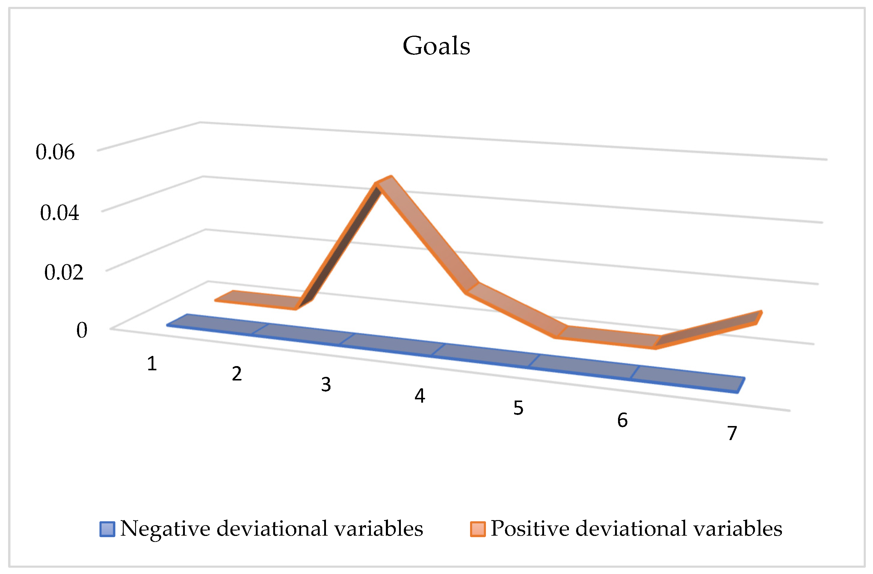
${\tau }_7$	$0$	$0.01185368$

and Figure 1 illustrate the possible progress toward the target worth using the optimal solution of the GP model. Three potential improvements can be made to the target. As a first step in detecting possible increments or decreases, positive values of deviation variables will be considered. For example, we can show that a positive deviation variable can be used to calculate the increment in the case of a maximization problem. For a minimization problem, however, a negative deviation variable can be used to calculate the decrease.

5. Discussion

As a result, the decrement can be determined by using a negative deviation variable. Finally, we interpreted these points according to their priority goals:

(i)

The company’s first goal is totally attained as $d_1^{-}$ and $d_1^{+}$ are zero, and it concluded that the company’s total assets for eleven years remain the same;

(ii)

Similarly, since $d_2^{-}$ and $d_2^{+}$ are zero, second goal is also achieved;

(iii)

The value of $d_3^{-}$ for goal three is zero, whereas $d_3^{+}$ is $0.04694982$. Thus, the company’s equity can increase by SAR 0.04694982 trillion annually after meeting the equity goal;

(iv)

For goal four, $d_4^{-}$ is zero, whereas $d_4^{+}$ is $0.01220811.$ Therefore, the company’s gross profit goal was reached, resulting in a yearly increase of SAR 0.01220811 trillion in gross profit;

(v)

Furthermore, because both $d_5^{-}$ and $d_5^{+}$ are equal to zero, maximizing total operating income for goal five is achieved. Therefore, total income remains the same for eleven years.;

(vi)

Furthermore, because $d_6^{-}$ and $d_6^{+}$ are equal to zero, goal six is also achieved by maximizing total net income. As a result, total net income remained constant for eleven years;

(vii)

As a final goal, the overall goal should be maximized. According to the results, $d_7^{-}$ is zero, while $d_7^{+}$ is 0.01185368, indicating that annual goal achievements can increase by SAR 0.01185368 trillion.

6. Conclusions

In recent years, researchers have focused on financial institutions’ financial planning to overcome the shortfalls seen in financial planning. This study evaluated SABIC’s financial performance; as a result, SABIC can accomplish all the goals outlined in this study based on the optimal solution to the developed model.

Consequently, SABIC can maximize its assets, equity, gross profit, and net income and achieve its overall goals. The study thus helps other financial institutions continue to improve by identifying updated benchmark values. In addition, this model allows financial institutions to develop strategies and make decisions based on varying economic conditions.

Future studies should examine how fiscal planning can reduce total liabilities while maximizing other objectives. Therefore, the results of this study will be crucial in overcoming future financial difficulties. In addition, future studies concerning performance management in financial institutions may also address this study’s findings. Furthermore, the proposed model will be applied to all Saudi financial institutions in subsequent research.

References

- Available online: https://www.sabic.com/en/about/corporate-profile (accessed on 10 June 2022).
- Available online: https://brandfinance.com/insights/brand-spotlight-sabic (accessed on 10 June 2022).
- Dan, E.D.; Desmond, O.O. Goal programming: An application to budgetary allocation of an institution of higher learning. Res. J. Eng. Appl. Sci. 2013, 2, 95–105. [Google Scholar]
- Farahat, F.A.; ElSayed, M.A. Achievement Stability Set for Parametric Rough Linear Goal Programing Problem. Fuzzy Inf. Eng. 2019, 11, 279–294. [Google Scholar] [CrossRef]
- Chowdary, B.V.; Slomp, J. Production Planning under Dynamic Product Environment: A Multi-Objective Goal Programming Approach; Department of Production Systems Design, Faculty of Management & Organization, University of Groningen: Groningen, The Netherlands, 2002; pp. 1–48. [Google Scholar]
- Lin, T.W.; O’Leary, D.E. Goal programming applications in financial management. Adv. Math. Program. Financ. Plan. 1993, 3, 211–230. [Google Scholar]
- Hotvedt, J.E. Application of linear goal programming to forest harvest scheduling. J. Agric. Appl. Econ. 1983, 15, 103–108. [Google Scholar] [CrossRef] [Green Version]
- Tamiz, M.; Jones, D.; Romero, C. Goal programming for decision making: An overview of the current state-of-the-art. Eur. J. Oper. Res. 1998, 111, 569–581. [Google Scholar] [CrossRef]
- Lam, W.S.; Lam, W.H.; Lee, P.F. Decision Analysis on the Financial Management of Shipping Companies using Goal Programming Model. In Proceedings of the 2021 International Conference on Decision Aid Sciences and Application (DASA), Sakheer, Bahrain, 7–8 December 2021; pp. 591–595. [Google Scholar]
- Romero, C. Extended lexicographic goal programming: A unifying approach. Omega 2001, 29, 63–71. [Google Scholar] [CrossRef]
- Kruger, M. A Goal Programming Approach to Strategic Bank Balance Sheet Management. In SAS Global Forum 2011 Banking; Financial Services and Insurance, Centre for BMI, North-West University: Potchefstroom, South Africa, 2011; pp. 1–11. [Google Scholar]
- Díaz-Balteiro, L.; Romero, C. Forest management optimization models when carbon captured is considered: A goal programming approach. For. Ecol. Manag. 2003, 174, 447–457. [Google Scholar] [CrossRef]
- Jamalnia, A.; Soukhakian, M.A. A hybrid fuzzy goal programming approach with different goal priorities to aggregate production planning. Comput. Ind. Eng. 2009, 56, 1474–1486. [Google Scholar] [CrossRef]
- Chen, J.W.; Lam, W.S.; Lam, W.H. Optimization on the financial management of the bank with goal programming model. J. Fundam. Appl. Sci. 2017, 9, 442–451. [Google Scholar] [CrossRef] [Green Version]
- Dyer, J.S. Interactive goal programming. Manag. Sci. 1972, 19, 62–70. [Google Scholar] [CrossRef]
- Kvanli, A.H. Financial planning using goal programming. Omega 1980, 8, 207–218. [Google Scholar] [CrossRef]
- ChiangLin, C.-Y. A Personal Financial Planning Model Based on Fuzzy Multiple Goal Programming Method. In Proceedings of the 9th Joint International Conference on Information Sciences (JCIS-06), Kaohsiung, Taiwan, 8–11 October 2006; pp. 129–132. [Google Scholar]
- Shafer, S.M.; Rogers, D.F. A goal programming approach to the cell formation problem. J. Oper. Manag. 1991, 10, 28–43. [Google Scholar] [CrossRef]
- Arewa, A.; Owoputi, J.A.; Torbira, L.L. Financial statement management, liability reduction and asset accumulation: An application of goal programming model to a Nigerian Bank. Int. J. Financ. Res. 2013, 4, 83. [Google Scholar] [CrossRef] [Green Version]
- Romero, C.; Rehman, T. Multiple Criteria Analysis for Agricultural Decisions; Elsevier: Amsterdam, The Netherlands, 2003; Volume 11, pp. 23–45. [Google Scholar]
- Schniederjans, M.J.; Hoffman, J.J.; Sirmans, G.S. Using goal programming and the analytic hierarchy process in house selection. J. Real Estate Financ. Econ. 1995, 11, 167–176. [Google Scholar] [CrossRef]
- Mirzaee, H.; Naderi, B.; Pasandideh, S.H.R. A preemptive fuzzy goal programming model for generalized supplier selection and order allocation with incremental discount. Comput. Ind. Eng. 2018, 122, 292–302. [Google Scholar] [CrossRef]
- Hoe, L.W.; Siew, L.W.; Fun, L.P. Optimizing the Financial Management of Electronic Companies using Goal Programming Model. J. Phys. Conf. Ser. 2021, 2070, 012046. [Google Scholar] [CrossRef]
- Choudhary, D.; Shankar, R. A goal programming model for joint decision making of inventory lot-size, supplier selection and carrier selection. Comput. Ind. Eng. 2014, 71, 1–9. [Google Scholar] [CrossRef]
- Schniederjans, M.J.; Wilson, R.L. Using the analytic hierarchy process and goal programming for information system project selection. Inf. Manag. 1991, 20, 333–342. [Google Scholar] [CrossRef]
- Lakshmi, K. Vasantha, Harish Babu GA, and Uday Kumar KN. Application of Goal Programming Model for Optimization of Financial Planning: Case Study of a Distribution Company. Palest. J. Math. 2021, 10, 144–150. [Google Scholar]
- Schniederjans, M.J.; Schniederjans, D.; Cao, Q. Value analysis planning with goal programming. Ann. Oper. Res. 2017, 251, 367–382. [Google Scholar] [CrossRef]
- AlArjani, A.; Alam, T. Lexicographic Goal Programming Model for Bank’s Performance Management. J. Appl. Math. 2021, 2021, 8011578. [Google Scholar] [CrossRef]
- Fechete, F.; Nedelcu, A. Multi-Objective Optimization of the Organization’s Performance for Sustainable Development. Sustainability 2022, 14, 9179. [Google Scholar] [CrossRef]
- Aouni, B.; McGillis, S.; Abdulkarim, M.E. Goal programming model for management accounting and auditing: A new typology. Ann. Oper. Res. 2017, 251, 41–54. [Google Scholar] [CrossRef]
Figure 1.
Outcomes of deviational variables.