Article

Experimental Modeling of a New Multi-Degree-of-Freedom Fuzzy Controller Based Maximum Power Point Tracking from a Photovoltaic System

by
Mohamed Fawzy El-Khatib
1,2,*,
Mohamed-Nabil Sabry
1,
Mohamed I. Abu El-Sebah
3,* and
Shady A. Maged
1
1
Mechatronics Engineering Department, Faculty of Engineering, Ain Shams University, Cairo 11517, Egypt
2
Mechatronics and Robotics Engineering Department, Faculty of Engineering, Egyptian Russian University, Cairo 11829, Egypt
3
Energy Conversion and Power Electronics Department, Electronics Research Institute, Cairo 11843, Egypt
*
Authors to whom correspondence should be addressed.
Appl. Syst. Innov. 2022, 5(6), 114; https://doi.org/10.3390/asi5060114
Submission received: 25 October 2022 / Revised: 5 November 2022 / Accepted: 8 November 2022 / Published: 12 November 2022
(This article belongs to the Section Control and Systems Engineering)

Abstract

:
Conventional control methods, which follow the maximum power point (MPP), suffer from being slow or inaccurate during sudden changes in irradiance and temperature. These problems can be solved using artificial intelligence algorithms. The current study proposes a new multi-degree-of-freedom (MDOF) fuzzy logic controller (FLC) for maximizing the overall output performance of a photovoltaic system. The MDOF-FLC was compared to the simplified universal intelligent PID controller (SUI-PID) using the MDOF concept and the normal FLC. Simulation and experimental results show that the proposed MDOF-FLC controller has a 37.8% and 58.1% faster response with a better rise time compared to the SUIPID controller and the normal FLC, respectively. At the same time, the error, measured by the integral time absolute error (ITAE), was 29.4% and 62.5% lower, respectively.

1. Introduction

Solar energy can power various applications, such as water pumping systems, especially in remote areas where electricity is unavailable. Additionally, they can provide water to metropolitan areas, reducing the reliance on fossil fuels for water pumping. Another application of solar energy is that it can be used for standalone electric vehicle charging [1]. PV-based water pumping systems may incorporate water storage towers to ensure water supply even on overcast days or at night. Numerous factors have a significant impact on the output power of photovoltaic panels. These variables include the irradiance level and temperature of the air. As a result, the amount of power supplied to the pump varies according to the season. Generally, there is a natural correlation between solar energy availability and the amount of water required. This is explained by increasing the water flow rate in hot weather when the solar irradiance is highest. The solar panel’s efficiency strongly depends on the irradiance and module temperature. As a result, an effective control system can maintain an optimal maximum power match across a range of radiation levels and operating temperatures. According to Thevenin’s theorem, to deliver the most significant amount of power from the PV panel to the load, the PV resistance should be equal to the load resistance for all operating conditions. MPPT control methods use a converter to modify the solar system’s operating point until the MPP is obtained. They adjust the duty cycle until the GMPP is obtained. As a result, the most incredible power given to the load is met, and the highest conversion efficiency is attained. The MPPT methods include both conventional and intelligent algorithms. Conventional methods employ a fixed step to determine the value of the duty cycle [1,2,3], which causes inaccurate tracking of power points under varying atmospheric conditions. Intelligent algorithms can employ a variable step size to determine the best value of the duty cycle, resulting in enhanced response time and stability under a wide range of operational circumstances [4,5,6,7,8,9,10].
Aldair et al. [5] pioneered using an adaptive neuro-fuzzy inference system (ANFIS) reference model. Additionally, they built a method of constant voltage and incremental conductance (IC) on a field-programmable gate array board to test and evaluate their performance. The results indicate that the ANFIS reference model is more effective and has a better dynamic response when compared to the IC and constant voltage techniques. Li et al. [6] improved the MPPT’s accuracy by proposing a new overall distribution (OD) algorithm that was combined with a particle swarm optimization (PSO) algorithm. They demonstrated that using the OD-PSO MPPT algorithm, the optimal particle positions for the PSO algorithm could be determined. Additionally, the OD-PSO algorithm outperformed conventional methods based on Firefly and PSO. Priyadarshi et al. [7] demonstrated a technique for three-phase voltage source inverter current control using fuzzy space vector pulse width modulation (FSVPWM). They achieved excellent tracking efficiency and optimal MPP in adverse operating conditions by utilizing a hybrid fuzzy particle swarm optimization technique. The results reveal more excellent performance when load and parameter fluctuations are nonlinear. Rocha et al. [11] proposed Hybrid Bat MPPT algorithms using established techniques like IC, beta, and perturbation and observation (P&O). They obtained more accurate results when solar irradiance and load varied slightly. Chandra et al. [12] presented an effective tracking of the MPP using a radial basis function neural network (RBFNN) for a water pumping system. The results indicate that the RBFNN MPPT algorithm more efficiently tracks MPP than the P&O and IC methods. Khatib et al. [13] proposed a new control algorithm (SUI-PID) for determining the MPP of a solar pump system working under various operational situations. The SUI-PID enhances the dynamic response compared to the FLC by 32.7%. Additionally, an increase in the water flow rate was achieved.
The present work proposes a new MDOF-FLC for the MPPT to improve the performance of the photovoltaic system. The proposed algorithm consists of two controllers: the first deals with significant errors (the fast controller), while the other deals with minor errors in the fine-tuning region (the slow controller). An error spike is caused by abrupt changes in temperature, irradiance, or both. The fast controller is preferred in transient conditions (regions where the error is significant), whereas the slow controller works in a steady state (areas where the error is minor). As a result, depending on the actual operating conditions, the MDOF-FLC combines the advantages of both rapid and slow controllers. The controller’s response is expected to be faster, with a better rise time and minimum overshoot. The performance of a BP SX 150S photovoltaic module under different types of DC pumping loads was simulated using MATLAB-Simulink.
The contributions of this paper can be summarized as follows:
  • Propose a new controller (MDOF-FLC) to extract the maximum power point from the photovoltaic system under different climatic conditions (temperature and/or irradiance).
  • Testing and evaluating the performance of the MDOF-FLC compared with the SUI-PID controller and the normal FLC under different solar pumps.
This paper will be structured as follows. Section 2 presents the overall system components as well as the mathematical modeling of the PV. Section 3 introduces the design of the converter. Section 4 and Section 5 show the controllers we are comparing, i.e., SUI-PID with the MDOF concept controller and the FLC controllers. The proposed controller, MDOF-FLC, will be discussed in Section 6. Section 7 presents the modeling and simulation of the solar pump. The theoretical and experimental results of the PV solar pump system are shown in Section 8 and Section 9, and the conclusions are given in Section 10.

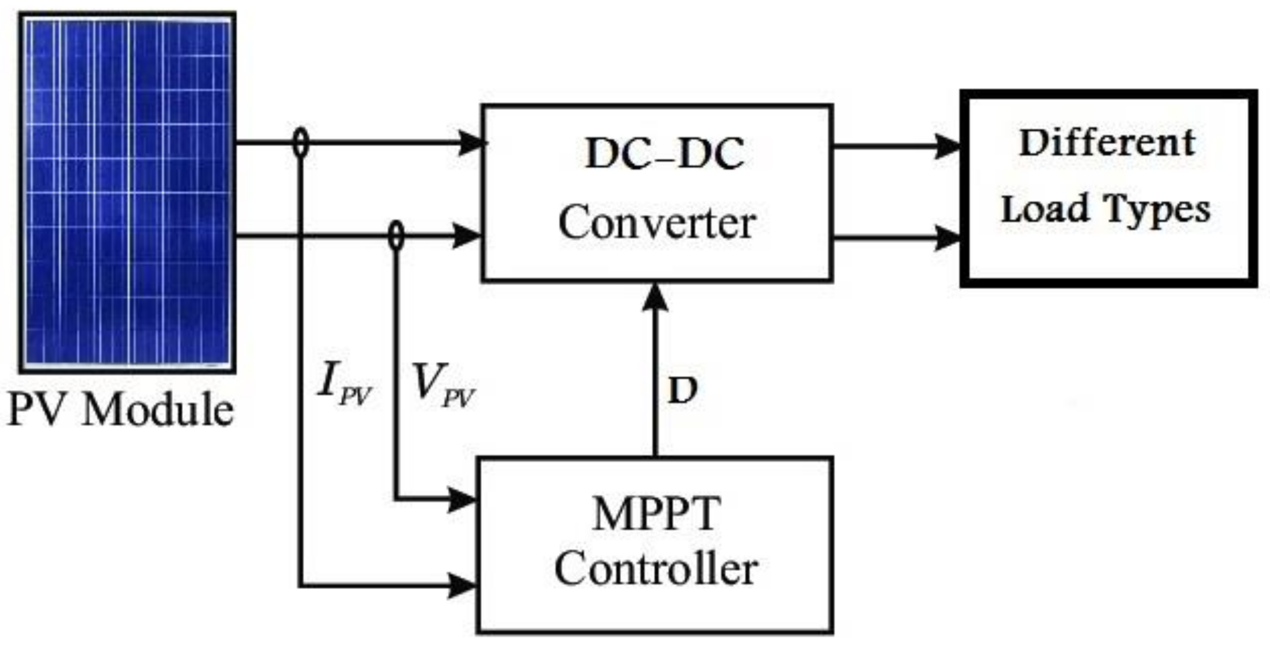
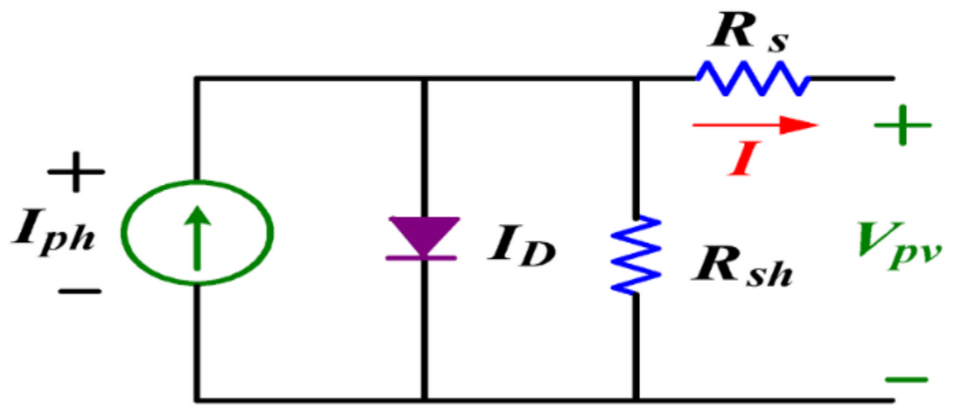
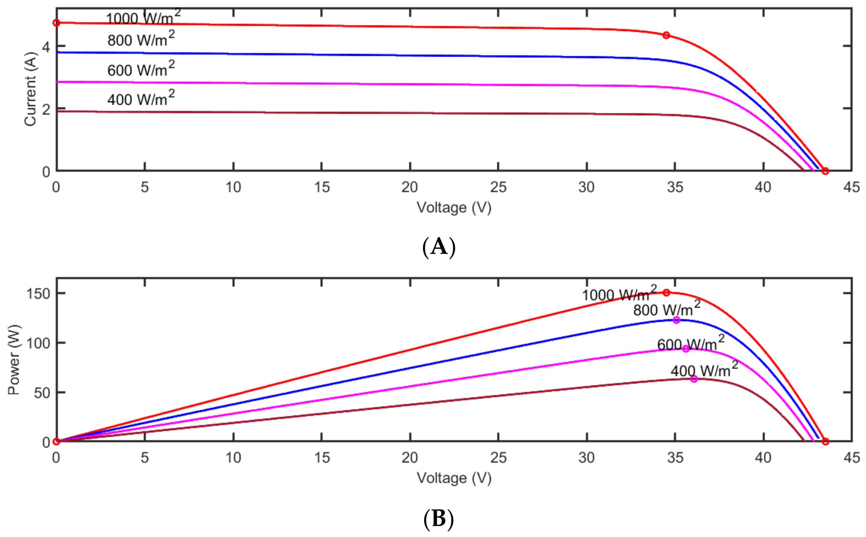
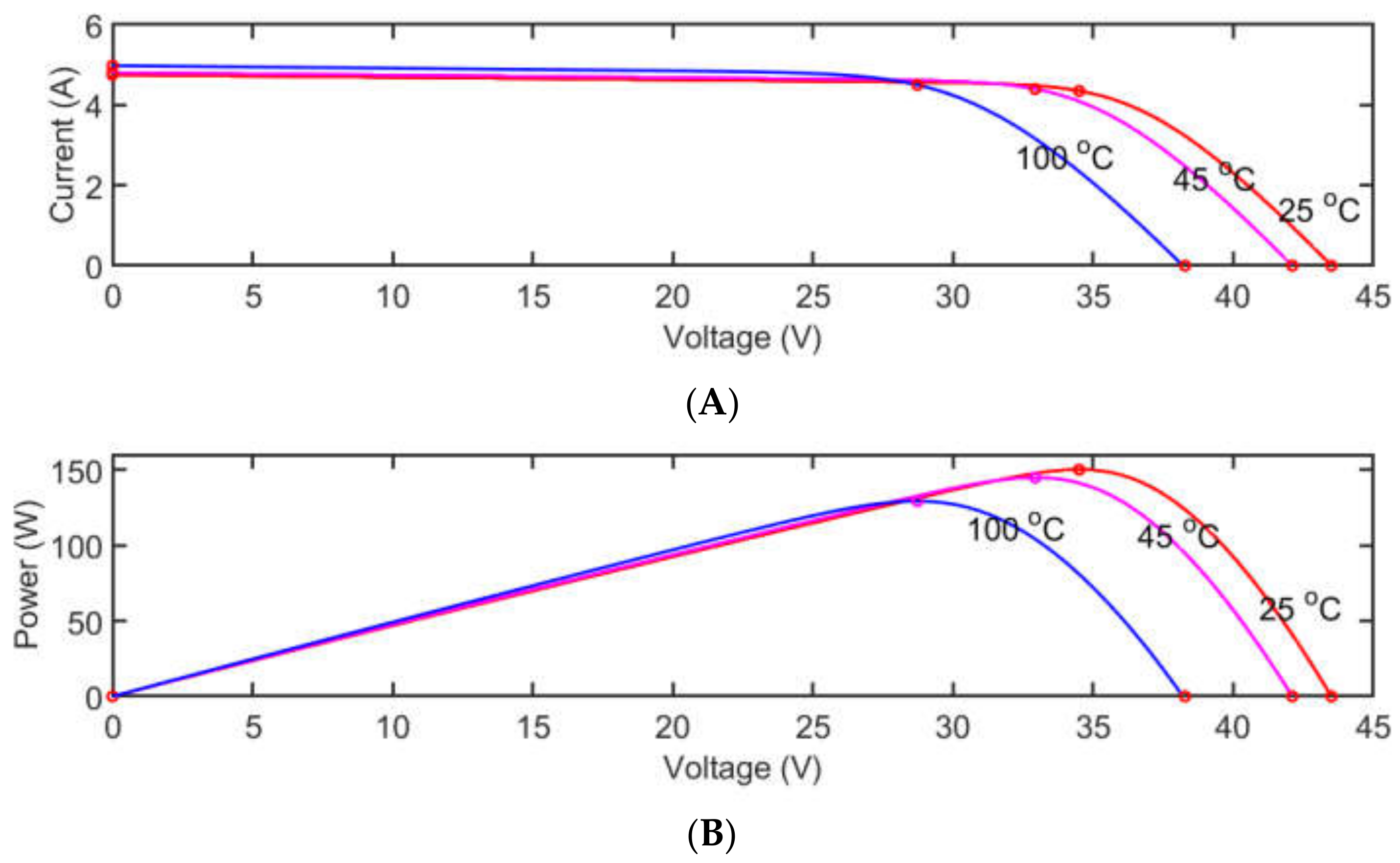
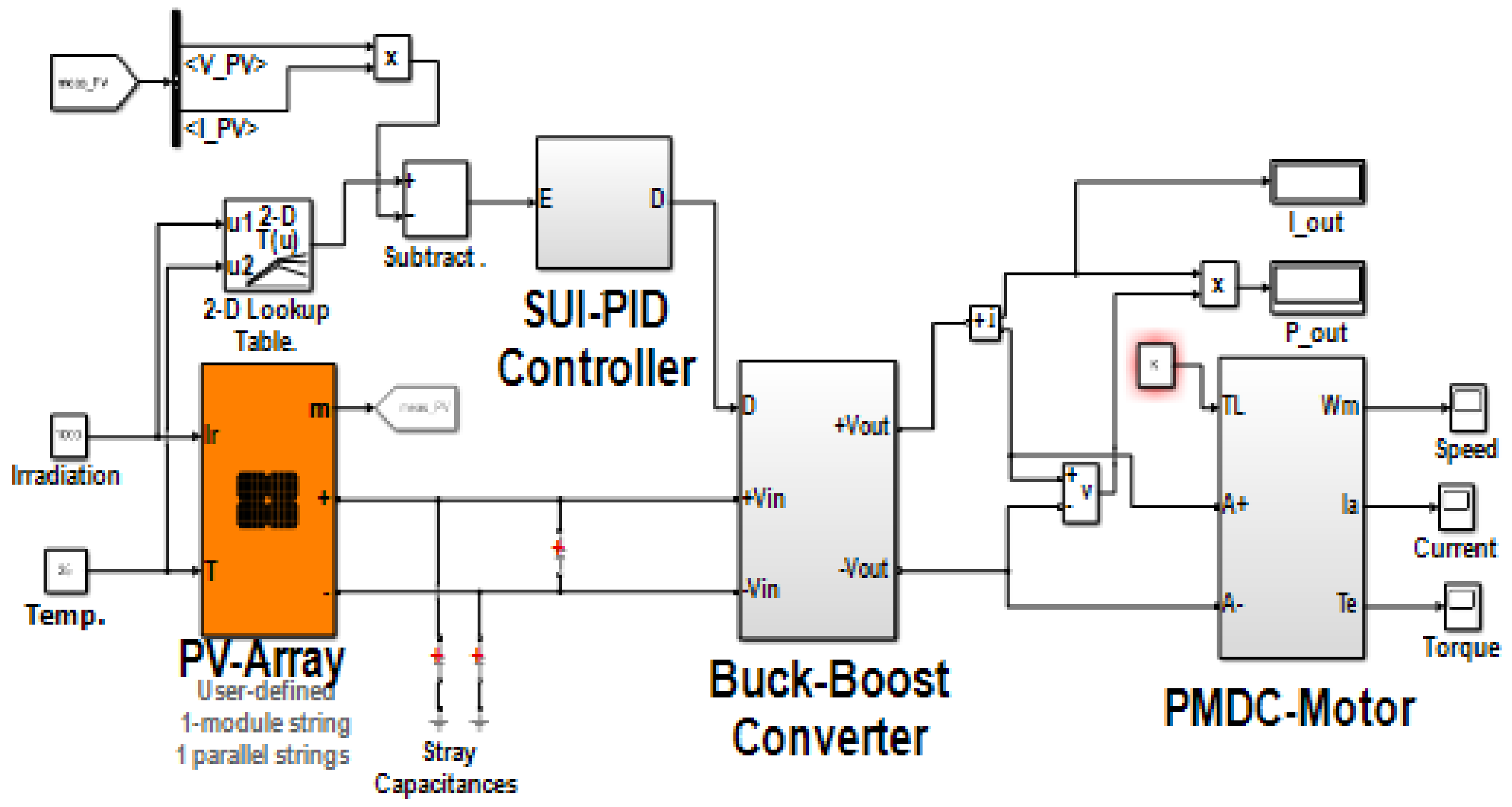
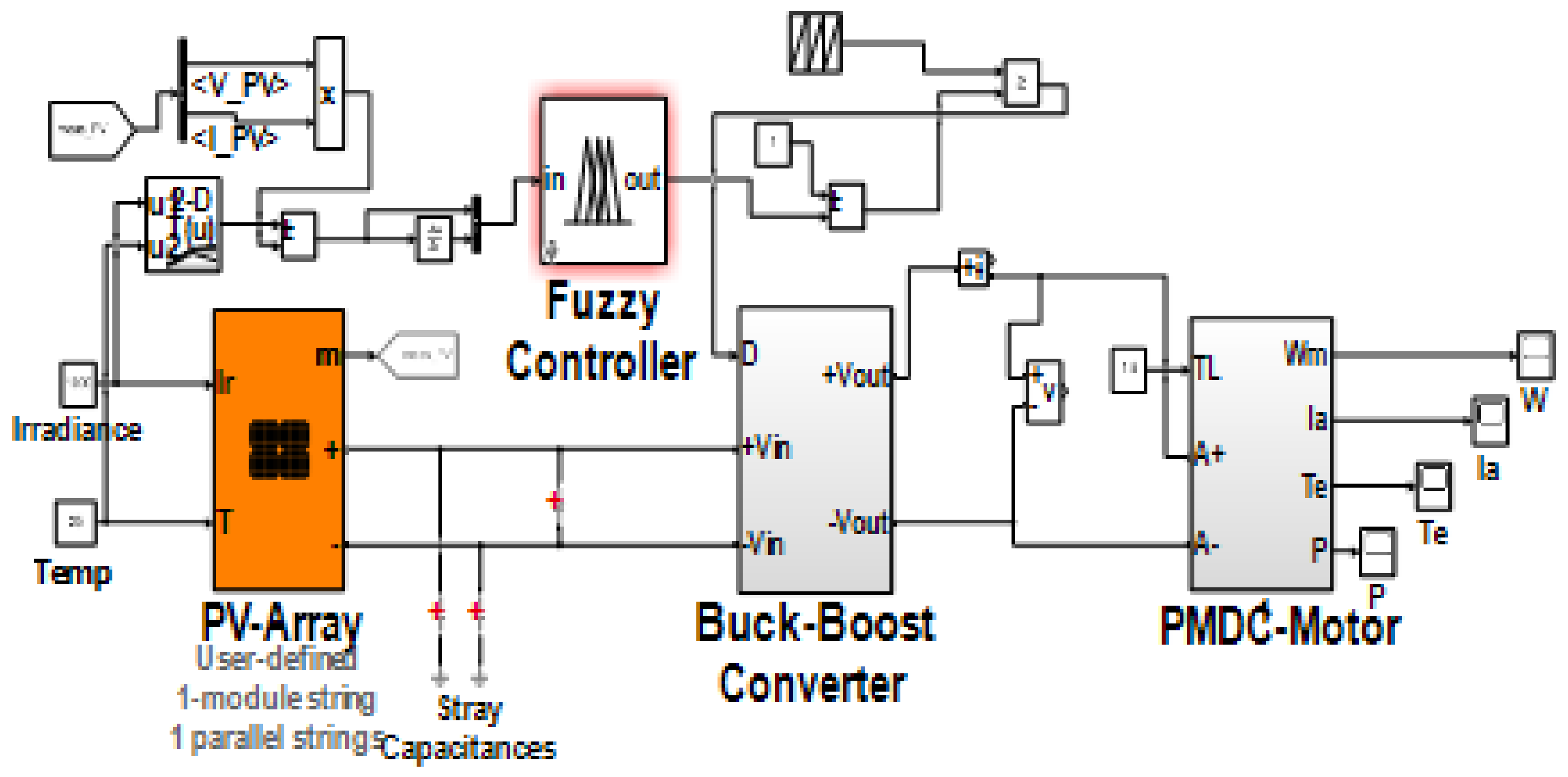
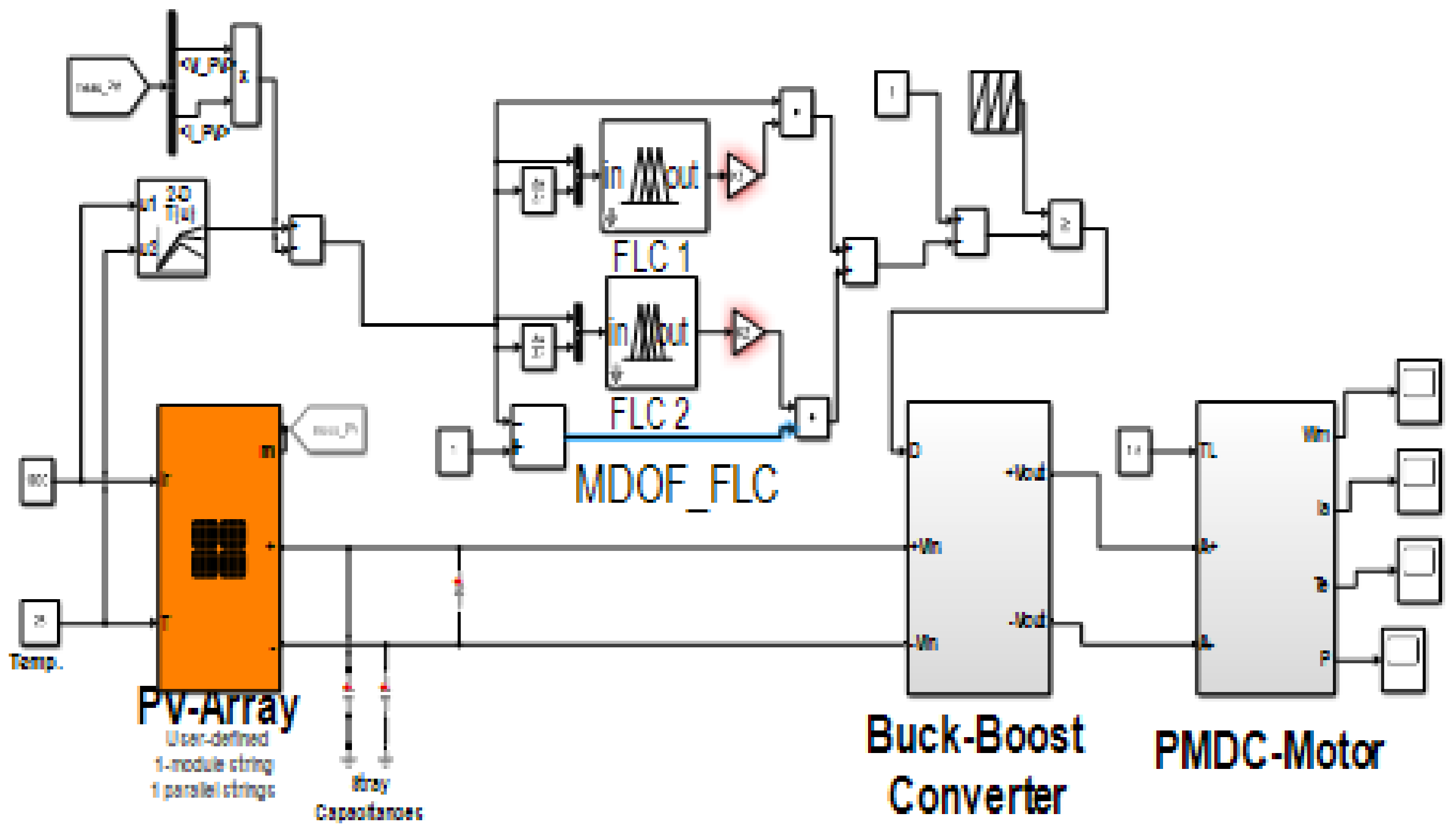
2. Modeling of the PV System

As illustrated in Figure 1, the photovoltaic system under investigation comprises three major components: a photovoltaic module, a direct current solar pump, and a MPPT control system. The MPPT system includes a look-up table to indicate the maximum possible power at any irradiance and temperature. It also comprises a controller that compares the desired power with the actual one and takes corrective measures by specifying the duty cycle of a buck-boost converter. The MPPT control systems are composed of an MPPT algorithm and a DC-DC buck–boost converter. The photovoltaic panel comprises photovoltaic cells, which operate via the photoelectric effect, arranged in series and parallel, as the potential generated by a single photovoltaic cell is small. The output voltage–current relationship in a photovoltaic cell is nonlinear. The equivalent circuit is based on a single-diode circuit model, as illustrated in Figure 2. The BP SX 150S solar module was chosen to power several pumps. Its parameters are listed in Table 1 [14,15,16].
By applying Kirchhoff’s current law, the output current of the solar cell can be calculated as
I = I p h I D I s h
I = I p h I S exp q V + R s K C A 1 V + R s R s h
I p h = I S C + K 1 ( T C T r ) λ
where I: overall output current from the cell; Iph: photocurrent generated by light; ID: current through the diode; ISh: current through the shunt resistor; IS: diode saturation current; K1: Boltzmann constant; q: electron charge; Tc: actual cell temperature; RSh: shunt resistance; ISC: short-circuit current; Tr: reference temperature; λ: irradiance; and RSh: series resistance.
Figure 3A,B illustrates the I-V and P-V characteristics at various irradiations and constant temperatures (T = 25 °C). Figure 4A,B shows the I-V and P-V relationships at different temperatures and constant irradiance levels (1000 Watts/meter2).

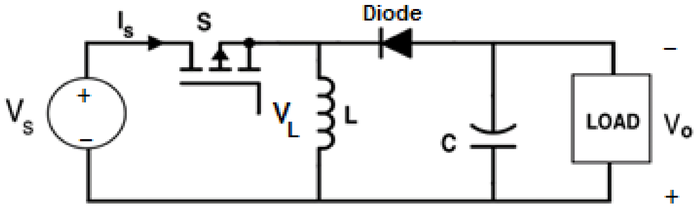
3. Design of Buck-Boost Converter

The converter can produce a varied output voltage range that may be larger or smaller than the actual input voltage [17,18,19,20,21]. The circuit diagram of the converter is shown in Figure 5. Its operation can be explained in two distinct modes: in the first mode, the power transistor is turned on, reversing the bias of the diode. As a result, the voltage across the inductor V L can be calculated as [13]
V L = V S
In the second mode, the power transistor will be turned off, allowing the stored current in the inductor to pass through the diode, capacitor, and finally to the load. Thus, the inductor voltage can be calculated as
V L = V o
Assuming a lossless circuit, the input and output voltages can be calculated as
V S D + V o ( 1 D ) = 0
D = t o n T
where the duty cycle is denoted by D, the switching time is ton, and the switching period is T. Thus, the input voltage and output voltage are described as
V o = D 1 D V S
The converter has a maximum output voltage of 45 V and a maximum power output of 160 W, so it can be used to power the Kyocera SD 3–70, SD 12–30, and SD 6–35 solar pumps. The converter was designed with the parameters shown in Table 2.

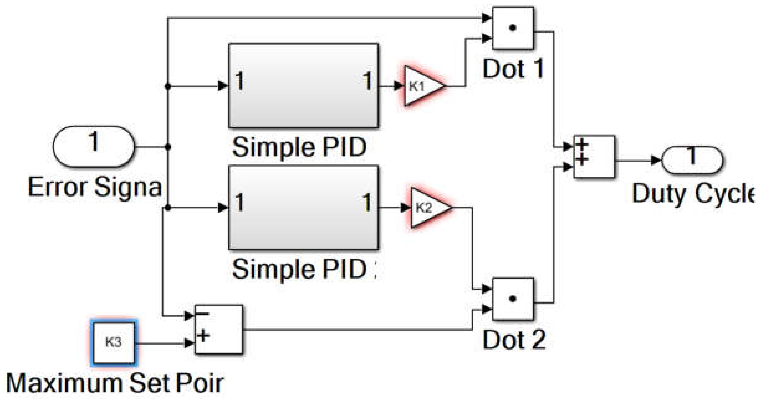
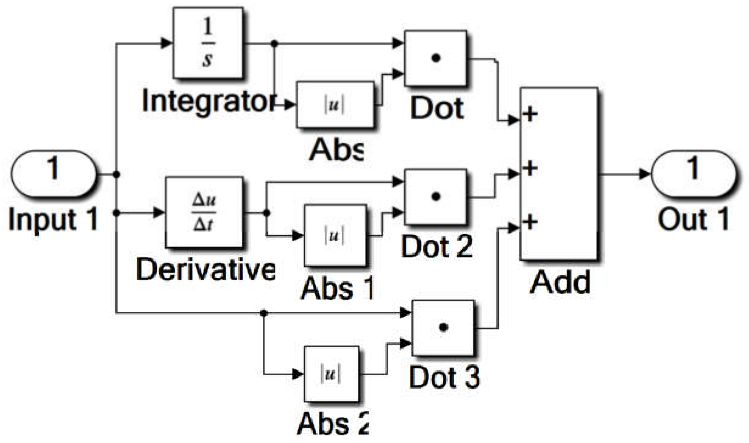
4. SUI-PID Controller

The SUI-PID implements the MDOF concept by utilizing two controllers. The first addresses large errors to achieve rapid error correction, while the second addresses small errors to achieve fine-tuning. The output can be calculated as [22,23]
Output = O / P 1 ( error ) + O / P 2 ( 1 error )
where O/P1 is the first controller’s output, which deals with the significant error, and O/P2 is the second controller’s output, which deals with the fine-tuning error.
Figure 6 illustrates the SUI-PID controller’s construction, in which two adaptive weights were added to the outputs of the two controllers, (1-error) and (error), resulting in an adequate tracking response. The design for each controller can be simplified by a PID controller, as shown in Figure 7, which has the following parameters:
K P = A b s ( e ) ; K i = A b s e ; K d A b s ( d e / d t )
Lastly, the output can be calculated as
C m = C K E + C ( 1 / K ) ( 1 E )
C m = C E [ K ( 1 / K ) ] + ( C / K )
For K ≫ 1
C m = C E K
where Cm: tuned controller output; E: error signal; K: controller gain; and C: controller output.
When the SUI-PID is used on a photovoltaic pumping system, the controller’s input and output are the error signal and duty cycle, and the error can be calculated as [13]
E r r o r = max .   p o w e r m e a s u r e d   p o w e r
The maximum output power can be estimated by evaluating the properties of the photovoltaic panel under various irradiation levels and temperatures, as shown in Figure 3. The system with the SUI-PID Simulink model is illustrated in Figure 8.

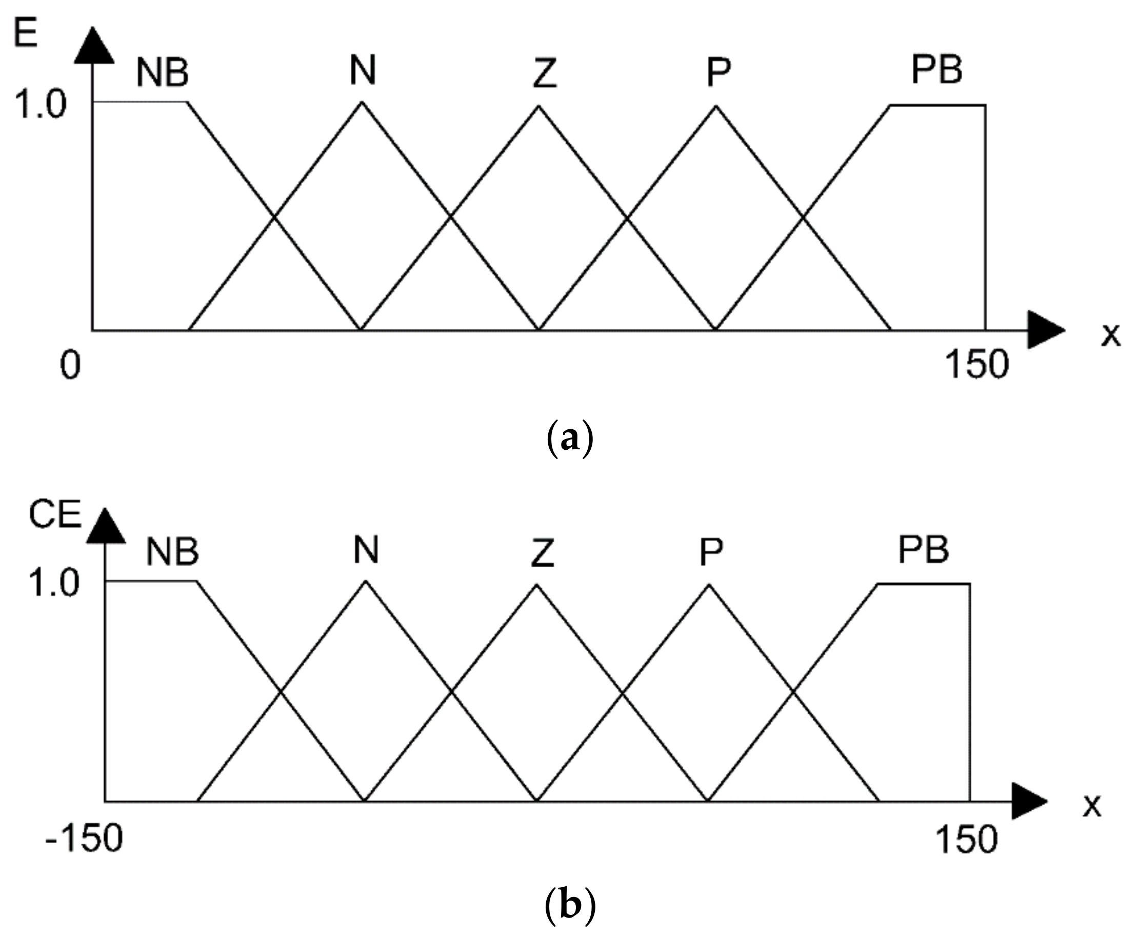
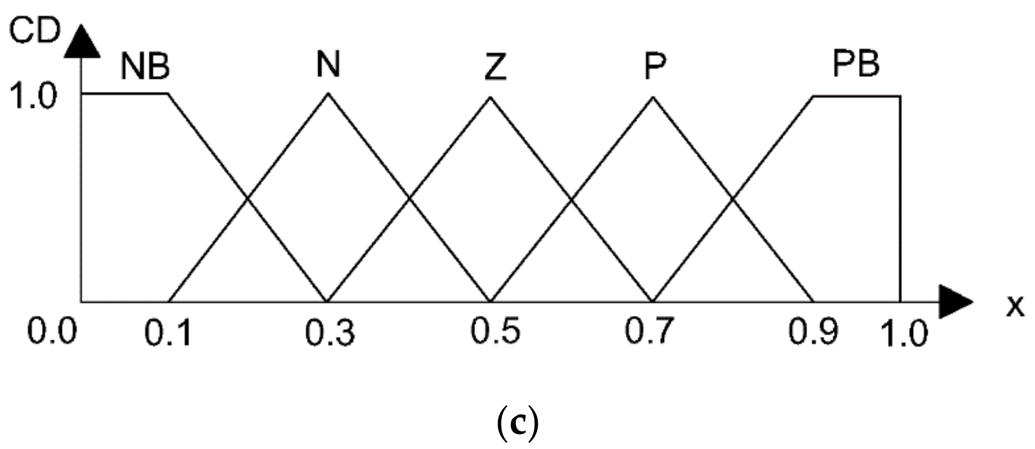
5. Normal Fuzzy Logic Controller

The FLC is an approach to attaining the MPP of photovoltaic systems based on an expert-type control method that uses human experience to make decisions. The fundamental concept is the use of language to specify control rules. The distinguishing feature is the transformation of human experience into control rules. Thus, fuzzy control is more advantageous when dealing with complex nonlinear systems whose mathematical model is unknown. Generally, the controller is divided into three phases: fuzzification, rule-based table, and defuzzification. In this study, a Mamdani type is presented as it is considered the most popular type, and the rules can be obtained from experienced human operators. At the same time, the Sugeno approach is suitable for generating fuzzy rules from a given input–output dataset. A membership function with a triangle form is employed due to its fewer complexes when splitting values (low, medium, and high) than other membership functions. When the controller is used with the PV pumping system, the inputs to the controller are error (E) and change in the error signal (CE). The controller’s output is the duty cycle (CD). Five fuzzy sets are used to describe each input and output variable: NB (Negative Big), N (Negative), Z (Zero), P (Positive), and PB (Positive Big) [16,17,18,19,20,21]. The following equations define the fuzzy controller’s inputs and outputs:
C E = E ( n ) E ( n 1 )
C D = f ( E , C E )
where E(n): is the present value of the error and E(n − 1): is the previous value of the error.
The maximum output power can be defined by examining the characteristics of the photovoltaic panel at various temperatures and irradiance levels. The simulation work is considered a membership function with a triangular shape. The membership of the input and output signals, which were designed using simulation data, is shown in Figure 9. Fuzzy rules consist of linguistic rules that relate fuzzy inputs to fuzzy outputs. These are based on an expert’s knowledge and comprehension of the system’s behavior, which is necessary to accomplish the control objectives. The fuzzy control rules comprise a series of IF-THEN statements that include all relevant information for the controlled parameters. The rules are designed to incorporate the following considerations:
  • If a positive change in the error signal is followed by a positive change in the change of the error signal, the chopper duty ratio must be raised. If the error signal variation is negative, the chopper ratio should be lowered.
  • If the error signal change is zero or very close to zero, which means it has reached its maximum, the chopper ratio should not change.
  • If a negative change in the error signal is followed by a positive change in the error signal, the chopper duty ratio must be lowered. If the error signal variation is positive, then the chopper ratio should be increased.
The design of the fuzzy rules can be illustrated in Table 3, and the system with the normal FLC Simulink model is shown in Figure 10.
Figure 9. Membership functions of the fuzzy system. (a) Error signal. (b) Change of error signal. (c) Change of duty cycle.
Asi 05 00114 g009aAsi 05 00114 g009b

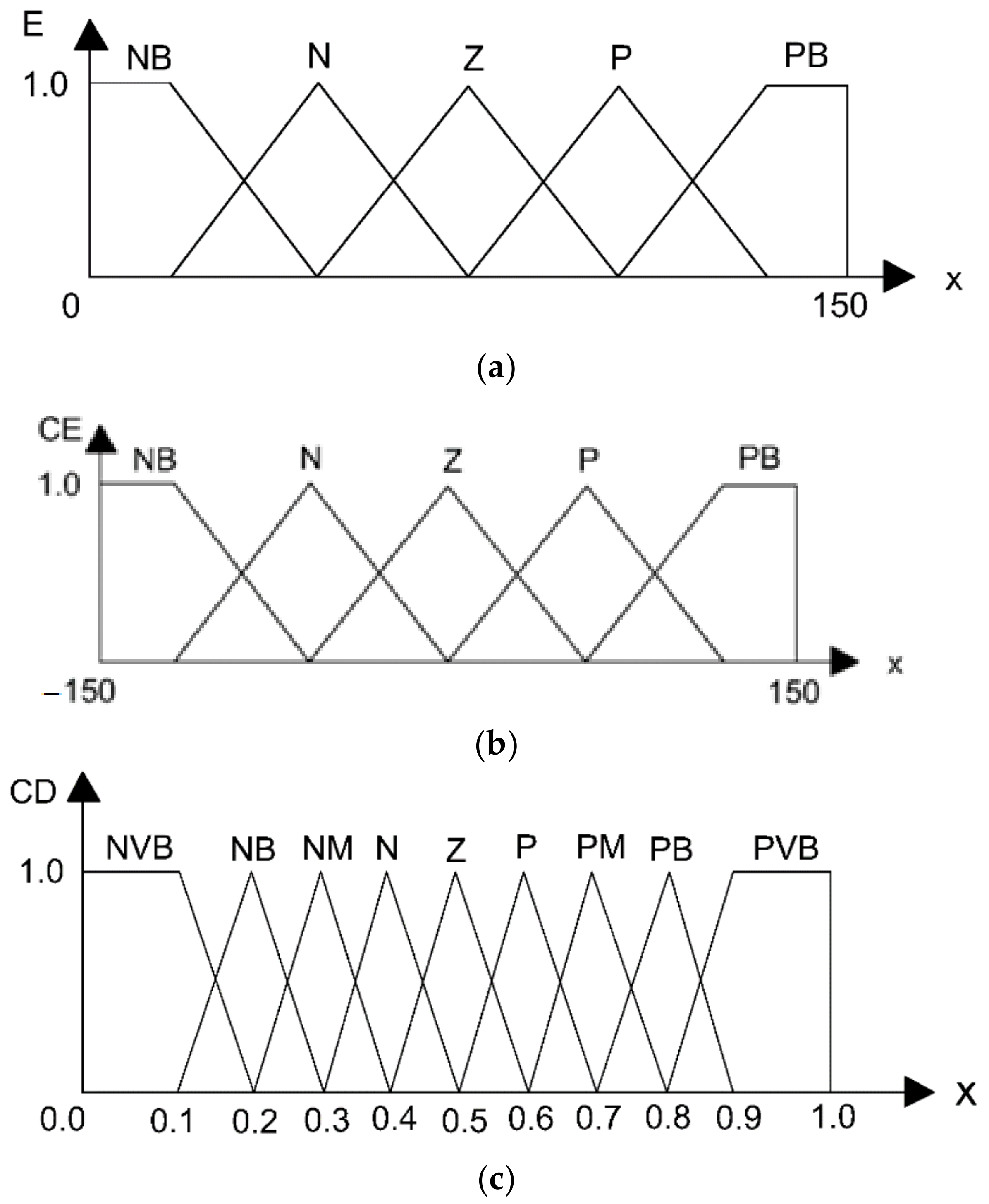
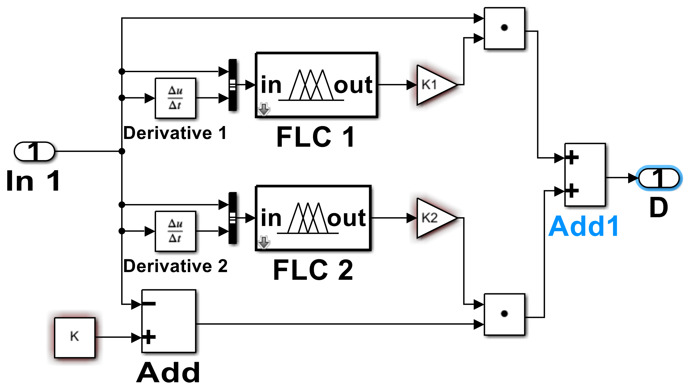
6. Design Methodology of the Proposed MDOF Fuzzy Logic Controller
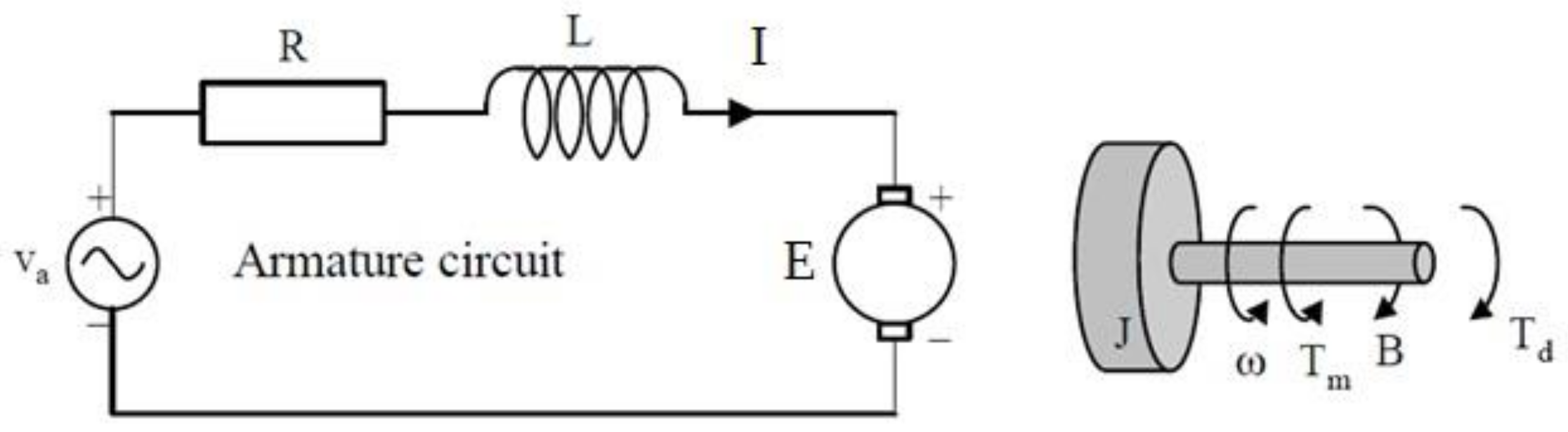
The MDOF concept applied to a fuzzy logic controller is the one proposed in this paper for the MPPT for a photovoltaic solar pump system. Numerous studies have employed the two fuzzy controllers as a two-degree-of-freedom controller, each controller being fired individually within a specific range [24,25]. This study introduces a novel method for creating a MDOF controller by combining two subcontrollers with distinct weights; the first is designed with a fast response to quickly deal with large errors, and the second controller deals with small errors for the fine-tuning region. The MDOF control can be applied to mix many specific controller outputs with different weights to produce the final MDOF controller output. The different controllers used may be designed with the same technique or different techniques to overcome many problems such as external disturbances and parameter variation. The design of the MDOF-FLC includes two steps:
Step 1
  • Fuzzy controller for the wide range of errors (faster controller): The faster fuzzy controller includes five fuzzy sets for the two inputs (E,CE) and five fuzzy sets for the output (CD), as shown in Figure 9, as well as Table 3.
  • Fuzzy controller for the fine-tuning controller (slow controller): It is similar to the preceding one, the main difference being using nine fuzzy output sets (Figure 11 and Table 4) to slow the output response to deal with the fine-tuning region.
Step 2
Implements the MDOF concept using Equation (9), which combines the outputs of the two subcontrollers with the two adaptive weights (1-error) and (error), resulting in an adequate tracking response, as shown in Figure 12. When using the MDOF-FLC on a PV pumping system, the controller’s inputs are the error signal, change in the error signal, and the duty cycle Equations (14)–(16). Figure 13 illustrates the system with the MDOF-FLC Simulink model.
Figure 11. Membership functions of the fuzzy system. (a) Error signal. (b) Change of error signal. (c) Change of duty cycle.
Asi 05 00114 g011

7. DC Solar Pump

Solar pumps are used in conjunction with photovoltaic systems to provide drinking and irrigation water. There are two types of pumps that are frequently used with photovoltaic systems: centrifugal and positive displacement pumps. For low-volume flow rates, a positive displacement type is used. Centrifugal pumps are more efficient and capable of pumping a high amount of water. However, these pumps require at least 600 watts of power. As a result, the present work proposes a positive displacement pump for use in standalone water delivery systems. The pump is connected to a permanent magnet DC motor due to its higher efficiency and ability to be directly coupled to a photovoltaic module. The motor’s equivalent circuit is illustrated in Figure 14 [26,27,28,29,30,31,32,33]
The PMDC motor’s mathematical model can be given by [13]
V a = R a I a + L a ( d I a / d t ) + K m W m
T e = K m I a
J ( d W m / d t ) = T e T L B m W m
where R denotes the resistance of the armature, L denotes the inductance of the armature, V a is the applied voltage, and W m is the motor rotational speed. K m : constant of torque, J denotes the inertia, B m denotes the viscous torque constant, T e denotes the electromagnetic torque, and T L denotes the load torque.
The amount of water pumped by the solar pump is determined by the pump’s efficiency, which is the ratio of its output hydraulic power to its input electric power [13]. The Kyocera DC solar pump can be directly connected to the PV system, as it consists of a DC motor connected to a positive displacement pump. The efficiency value is 40%, and the electrical parameters of the PMDC motor and the load are reported in Table 5 [13].
η P = ρ g h Q I V
where I: input current to the pump;   η p : pump efficiency; Q: Water flow rate; V: Applied voltage; ρ : density of water; g: acceleration of gravity; and h: Head.

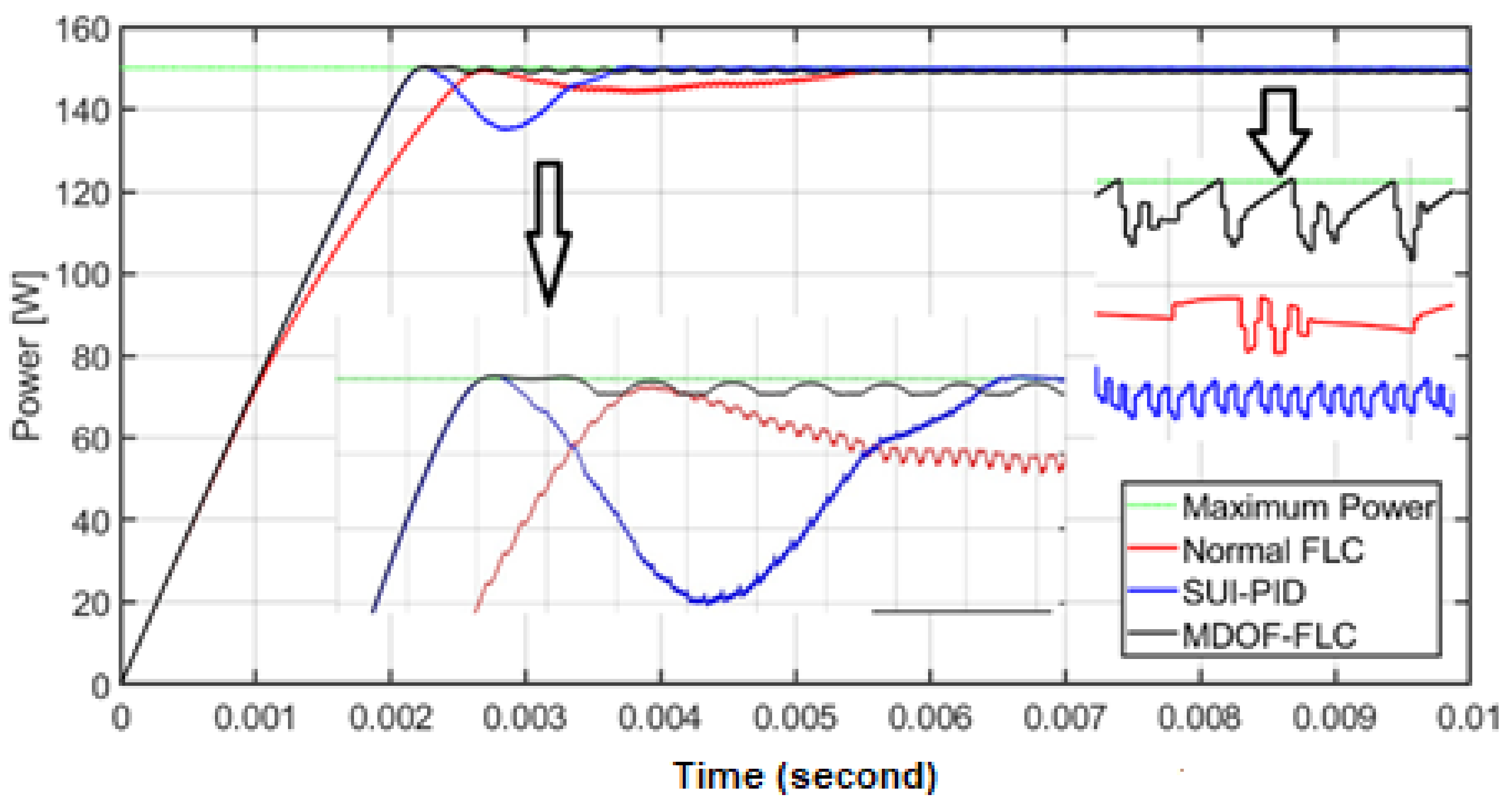
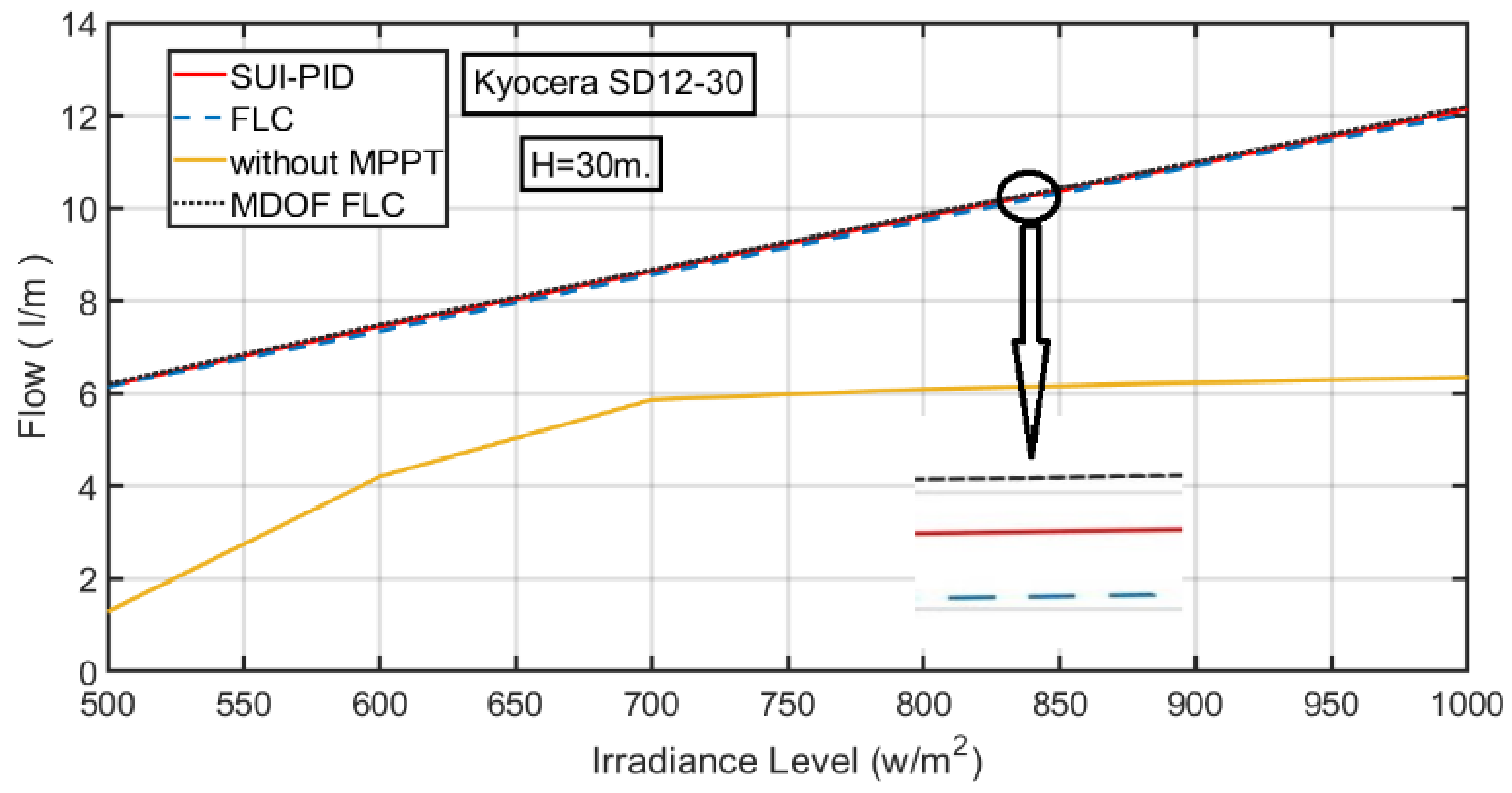
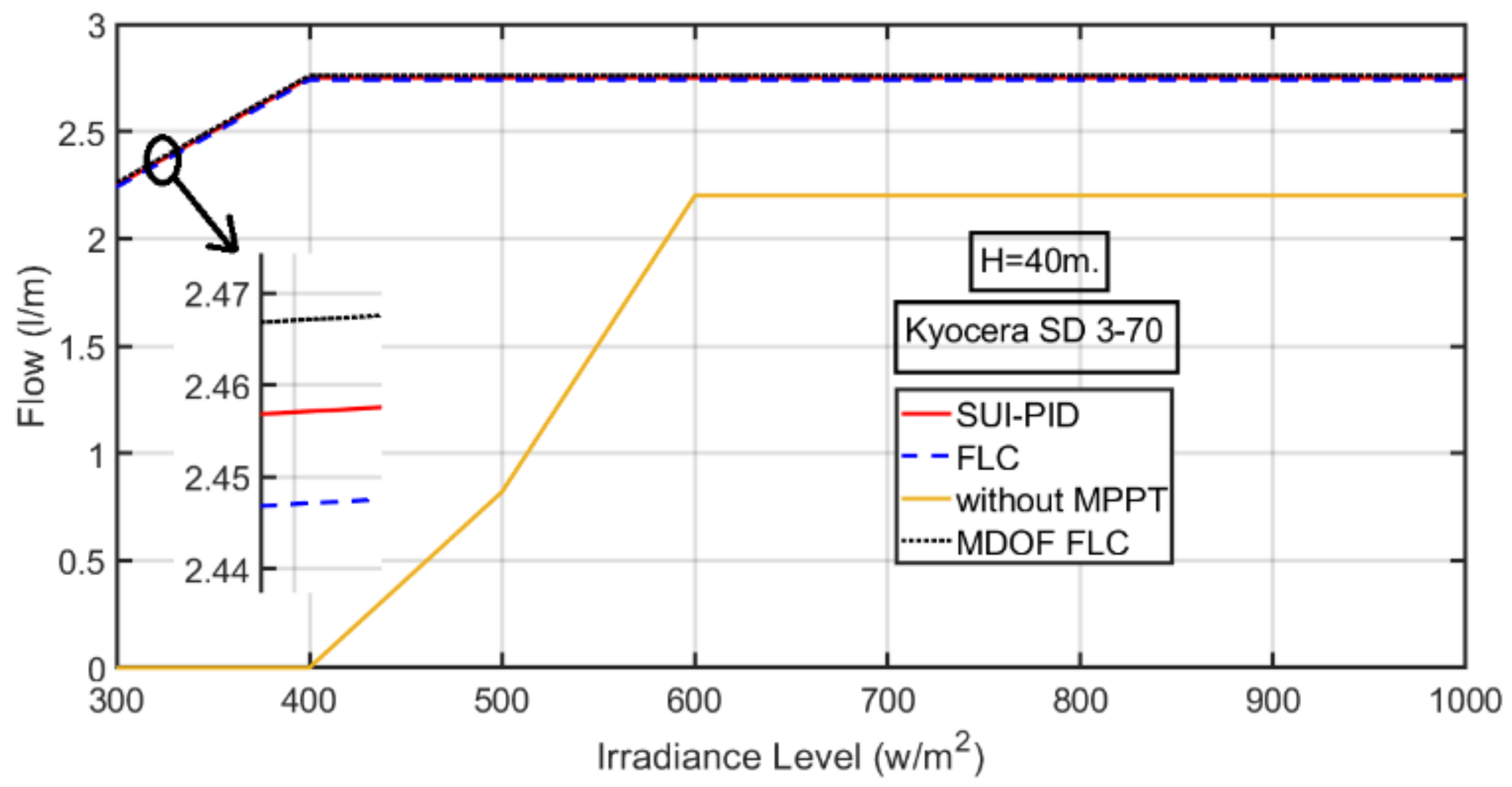
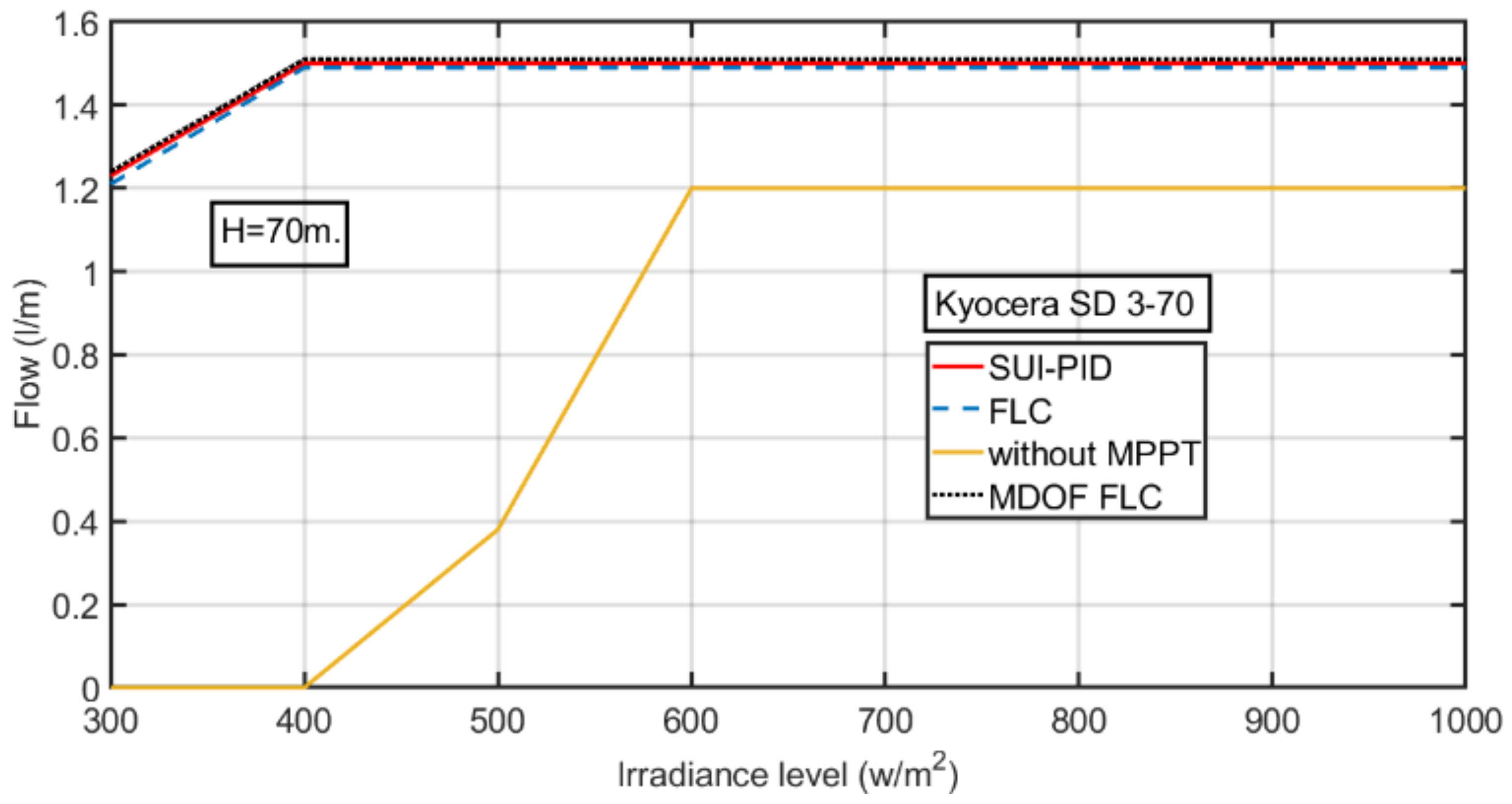
8. Theoretical Results

Figure 15 shows a comparison of the power delivered to the pump by the three controllers when the irradiance level is constant at 1000 Watt/m2 (the comparison includes constant step input as in Figure 15 and varying step input as in Figure 16). In comparison to the SUI-PID and the normal FLC controllers, the MDOF-FLC has a faster response, a better rise time, and a lower error. It appears from Table 6, showing the comparative performance analysis associated with different controllers, that the proposed MDOF-FLC records the best values in rising time, settling time, and integral time absolute error (ITAE). The time required to attain a steady state was 2.3 milliseconds with the MDOF-FLC, 3.7 milliseconds with the SUI-PID controller, and 5.5 milliseconds with the normal FLC. (i.e., 37.8% and 58.1% enhanced response compared to the SUI-PID controller and the normal FLC, respectively). Also, the error, measured by the ITAE, was 29.4% and 62.5% lower, respectively. Figure 16 illustrates the capability of the MDOF-FLC, normal FLC, and SUI-PID controllers to track the MPP under various irradiance levels. The irradiance level was abruptly increased from 600 Watt/m2 to 800 Watt/m2, and subsequently to 1000 Watt/m2. The three controllers responded well when following the MPP. However, the MDOF-FLC has a smaller rise and settling time.
Pump performance under a range of operating circumstances was simulated. These situations include varying scenarios, constant irradiance levels, and abrupt irradiance level fluctuations from 300 Watt/m2 up to 1000 Watt/m2 for all pumps. The pump performance curve [27] can be used to estimate the volume flow rate Q. The study analysis of the solar pump includes three different types: Kyocera SD (6–35), SD (12–30), and SD (3–70). The SD (6–35) was studied for heads of 15 m and the pump’s maximum water head of 35 m. Figure 17 and Figure 18 provide a comparative analysis of the amount of water for the heads under varied levels of irradiation using the proposed MPPT MDOF-FLC, MPPT FLC, MPPT SUI-PID, and without MPPT control. Next, the SD (12–30) was evaluated at heads of 20 m and the pump’s maximum water head of 30 m. Figure 19 and Figure 20 provide a comparative analysis of the amount of water for the heads under varied irradiance levels with the proposed MPPT-MDOF-FLC, the MPPT normal FLC, the MPPT SUI-PID, and without MPPT control. Finally, the SD (3–70) was evaluated at heads of 40 m and the pump’s maximum water head of 70 m. Figure 21 and Figure 22 provide a comparative analysis of the amount of water for the heads under varied levels of irradiation using the proposed MPPT MDOF-FLC, MPPT FLC, MPPT SUI-PID, and without MPPT control. Figure 23, Figure 24, Figure 25 and Figure 26 demonstrate an increase in the amount of water provided at various irradiance levels when the MPPT control algorithms are used. The proposed MDOF-FLC provides a slight increase in the water flow rate compared to the FLC.

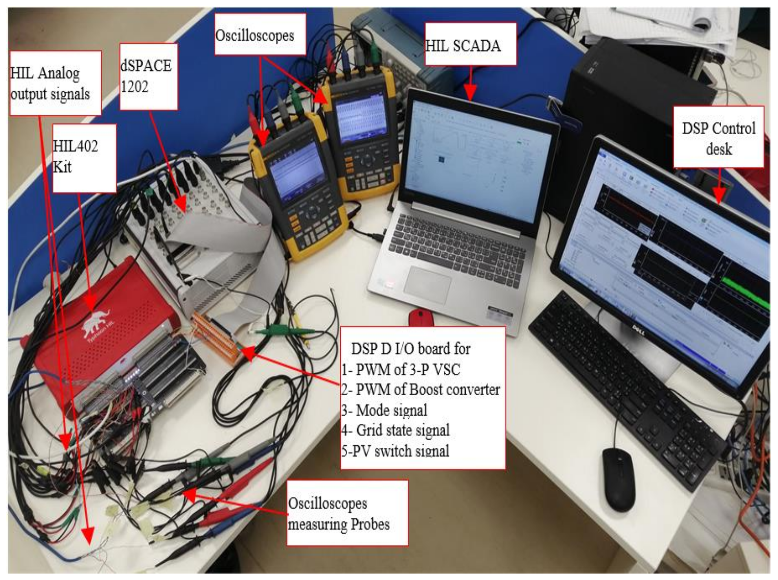
9. Experimental Setup

The experiment studies will be used to validate the proposed algorithm under a loading pump. The simulations in this study were conducted using MATLAB-implemented systems, and the experimental work was performed to confirm the simulation results under the same conditions. The experimental setup includes the MicroLabBox dSPACE1202 platform, which conducts the proposed MDOF-FLC, SUI-PID, and normal FLC with a sampling time of 0.0001 s. Typhoon HIL-402 was used to emulate the hardware configuration specified in [28], and the experimental setup of the system is illustrated in Figure 23.
Figure 24A,B,C displays the PV system’s experimental output power and voltage results with the proposed MDOF-FLC, SUIPID, and the normal FLC under constant atmospheric conditions (T = 25 °C, G = 1000 watts/m2). The figures pass from no control action mode (region part 1) to control action mode (region part 2). The no control action mode means that a constant duty cycle is applied to the converter in case the control action mode does not go on. Every division represents 100 watts for the power curve; for the voltage curve, every division represents 100 volts. The maximum output power from the PV module is 150 watts under conditions of a temperature of 25 °C and irradiation of 1000 Watt/m2. The experimental results, Figure 24A, show that the power curve has about 1.5 divisions * 100 watts (HIL probe) * 1 watt/div (scope probe) = 150 watts, approximately. The voltage curve shows 0.18 divisions * 100 volts/div (HIL probe) * 2 Volts/div (scope probe) = 0.18 * 2 * 100 = 36 V, the maximum output voltage of the module. The results show steady power and voltage levels for all controllers under uniform irradiance and temperature levels. However, the MDOF-FLC has fewer oscillations in the power level during constant atmospheric conditions compared to the SUI-PID and FLC.
Figure 25A–C displays the effects of increasing or decreasing irradiance levels with the proposed MDOF-FLC, SUIPID, and normal FLC, respectively, on the PV output power and voltage. The irradiance levels change from 1000 Watt/m2 (region 2) to 500 Watt/m2 (region 3), and finally back to 1000 Watt/m2 (region 4), and region 1 represents the no control action mode. The results show an excellent ability to track the MPP under varying irradiance levels with the three controllers. The voltage level remains steady under varying irradiance levels for all controllers. However, the MDOF-FLC has fewer oscillations in the power level during the variation in the irradiance levels compared to the SUI-PID and the FLC.
Figure 26A–C displays the effects of increasing or decreasing the temperature levels with the proposed MDOF-FLC, SUIPID controller, and normal FLC on the PV output power and voltage. The temperature levels change from 25 °C (region 1) to 35 °C (region 2), then 45 °C (region 3), and finally back to 25 °C (region 4). The results show an excellent ability to track the MPP under varying irradiance levels with the three controllers. The power level remains steadier under varying temperature levels with the MDOF-FLC controller compared to the SUI-PID and normal FLC.

10. Conclusions

A new MPPT control algorithm was applied to get the MPP from a PV system. Under different operating conditions, the MPPT of the system was studied using different controllers. These controllers are the proposed MDOF-FLC, the SUI-PID controller, and the normal FLC to validate the proposed controller. The simulations in this study were conducted using MATLAB-implemented systems. The experimental work was performed to confirm the simulation results under the same conditions using the MicroLabBox dSPACE1202 platform, which performs the three controllers. Typhoon HIL-402 was used to emulate the hardware configuration. Simulation and experimental results show that the proposed MDOF-FLC controller has a 37.8% and 58.1% faster response with a better rise time compared to the SUIPID controller and the normal FLC, respectively. At the same time, the error, measured by the integral time absolute error (ITAE), was 29.4% and 62.5% lower, respectively. Also, the following conclusions can be extracted:
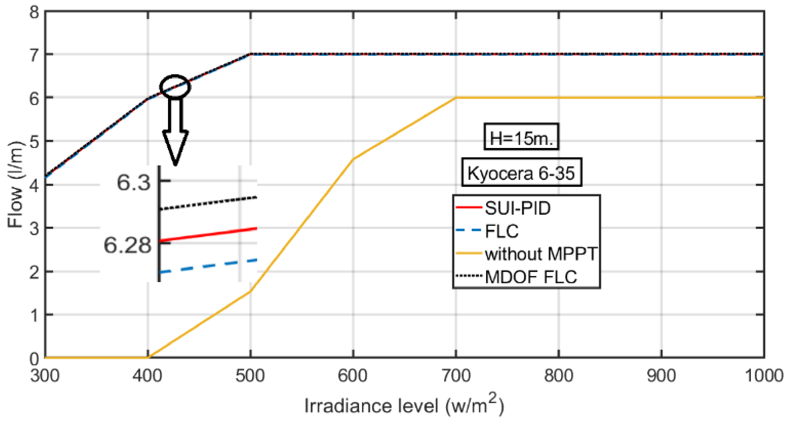
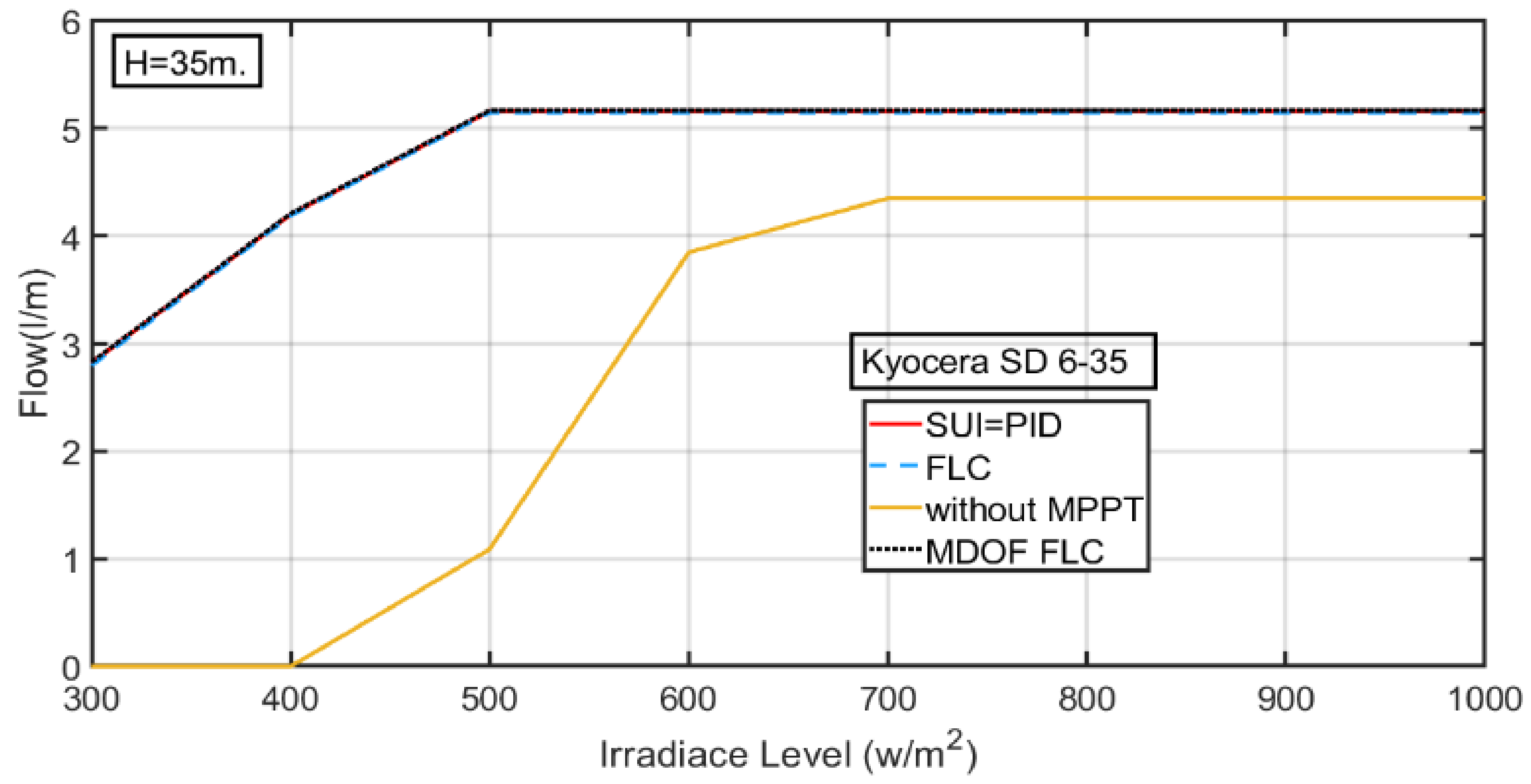
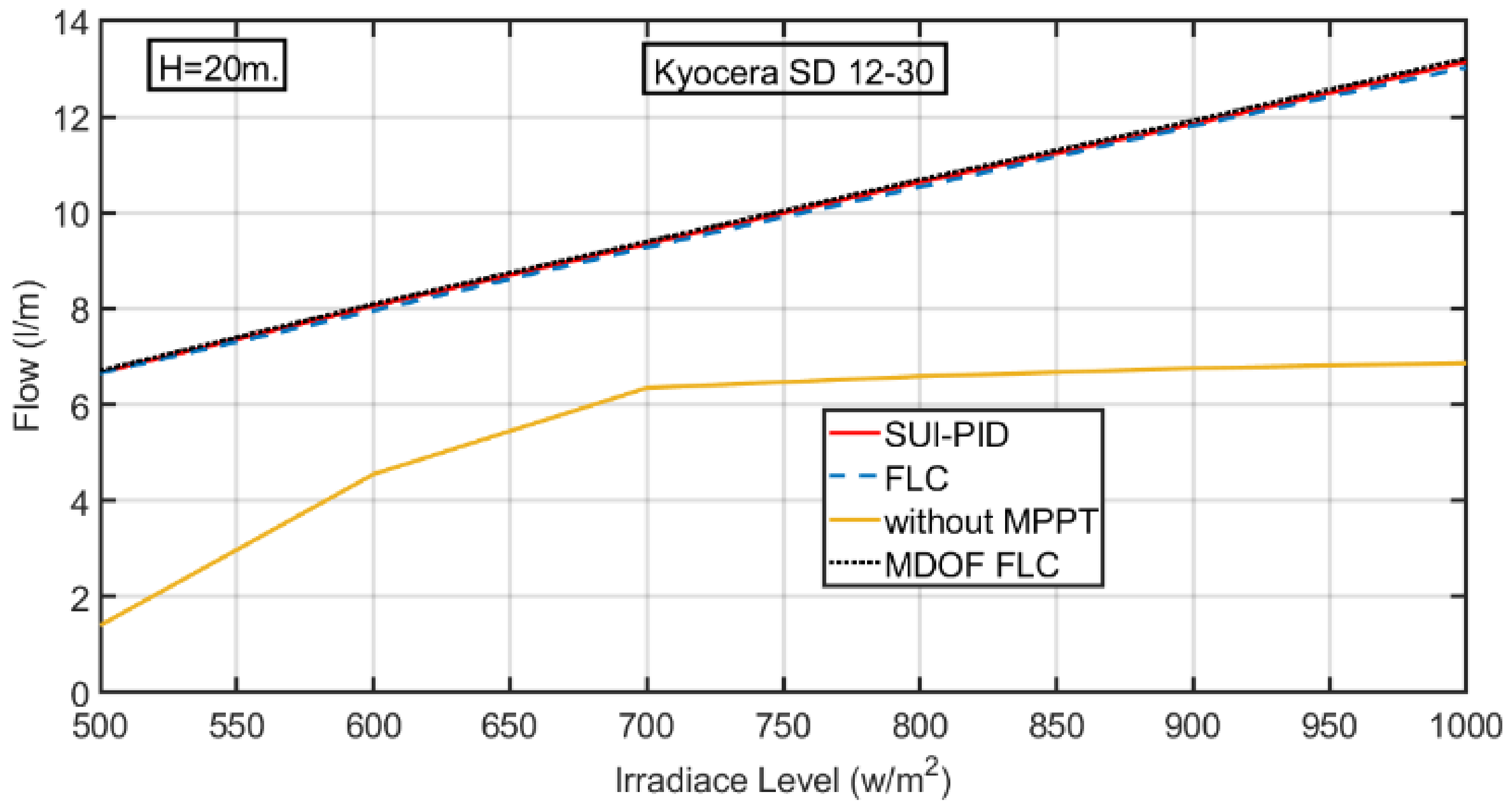
  • The MPPT control algorithms increased the water supply flow rate at various irradiance levels. However, the MDOF-FLC has provided a slightly higher water flow rate than the SUI-PID and the FLC.
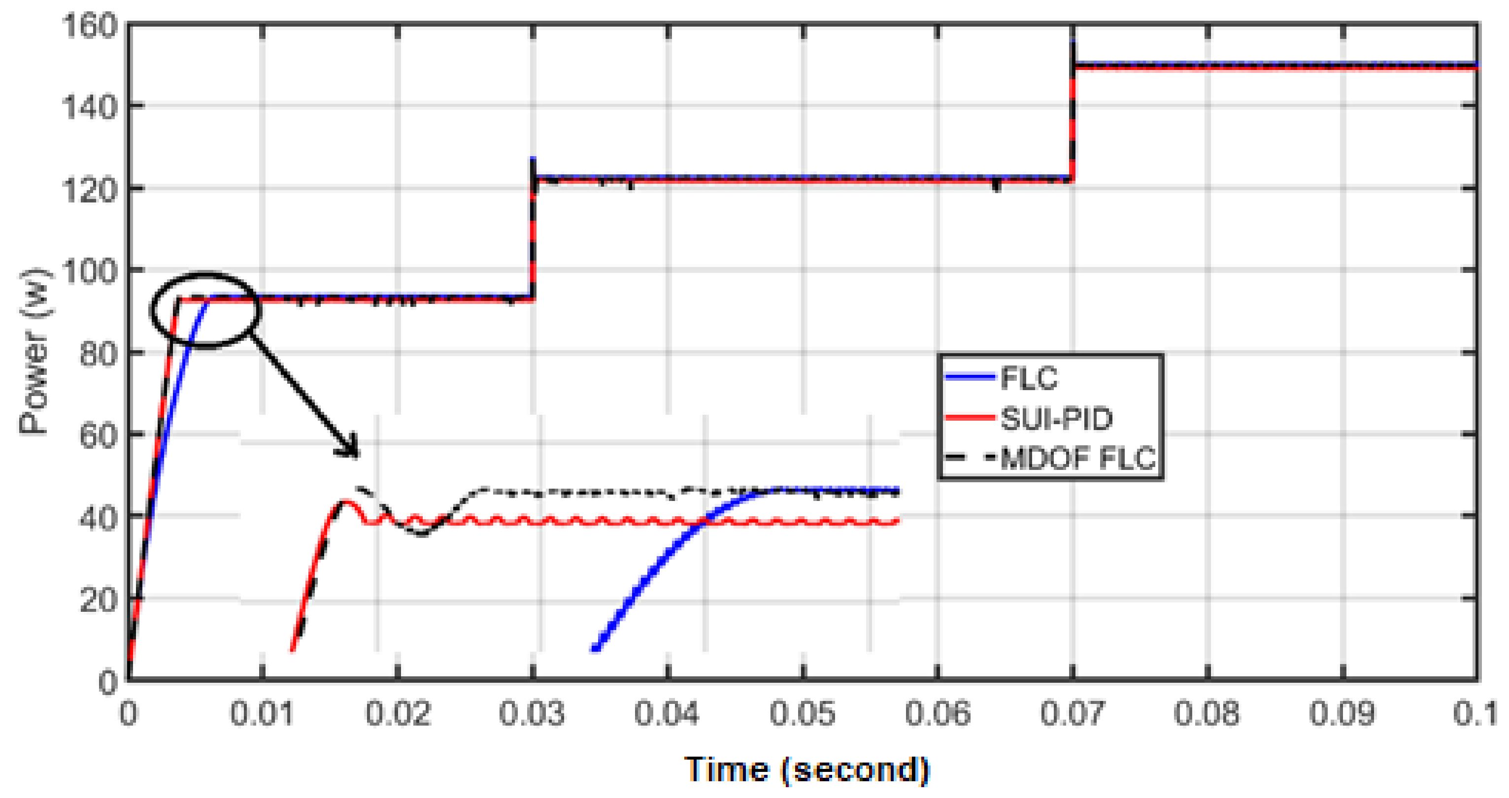
  • The MDOF-FLC provided a faster response and a better rise time. The MDOF-FLC reached a steady state at 2.3 milliseconds, the SUI-PID controller at 3.7 milliseconds, and the FLC at 5.5 milliseconds.
  • The MDOF-FLC, the SUI-PID controllers, and the normal FLC have a superior ability to track the PV panel MPP under sudden changes in irradiance levels and temperatures.
  • The MDOF-FLC is more suitable in the PV array or PV station system, which provides stable electricity for homes or other applications. It has more stability and a better rise time, resulting in a more efficient and accurate process.
In future work, the study and analysis of the stability of the proposed MDOF-FLC will be considered, as it is one of the essential concepts in the analysis and design of control systems. The study of the stability of fuzzy control systems has been complex since fuzzy systems are nonlinear systems. Recently, stability analysis techniques based on nonlinear stability theory have been developed and need further study. In addition, study the effect of the partial shading conditions on the PV system to evaluate the proposed controller compared with other intelligent controllers. Also, it is possible to use another type of microcontroller, such as Arduino, instead of the MicroLabBox dSPACE1202 platform, as it is simpler to perform the three controllers.

Author Contributions

Conceptualization, M.F.E.-K. and M.-N.S.; methodology, M.F.E.-K.; software, M.F.E.-K.; validation, M.F.E.-K. and M.I.A.E.-S.; formal analysis, M.F.E.-K.; investigation, M.F.E.-K.; resources, M.F.E.-K.; data curation, M.F.E.-K.; writing—original draft preparation, M.F.E.-K.; writing—review and editing, M.F.E.-K., M.-N.S., M.I.A.E.-S. and S.A.M. visualization, M.F.E.-K.; supervision, M.-N.S., M.I.A.E.-S. and S.A.M.; project administration, M.F.E.-K.; funding acquisition, M.F.E.-K. All authors have read and agreed to the published version of the manuscript.

Funding

This research received no external funding.

Institutional Review Board Statement

Not applicable.

Informed Consent Statement

Not applicable.

Data Availability Statement

Not applicable.

Conflicts of Interest

The authors declare no conflict of interest.

References

  1. Zaid, S.A.; Albalawi, H.; Alatawi, K.S.; El-Rab, H.W.; El-Shimy, M.E.; Lakhouit, A.; Alhmiedat, T.A.; Kassem, A.M. Novel Fuzzy Controller for a Standalone Electric Vehicle Charging Station Supplied by Photovoltaic Energy. Appl. Syst. Innov. 2021, 4, 63. [Google Scholar] [CrossRef]
  2. Liu, L.; Meng, X.; Liu, C. A review of maximum power point tracking methods of PV power system at uniform and partial shading. Renew. Sustain. Energy Rev. 2016, 53, 1500–1507. [Google Scholar] [CrossRef]
  3. Khemliche, M.; Bouamama, B.O.; Bacha, S.; Villa, L.F.L. Bond graph modeling and optimization of photovoltaic pumping system: Simulation and experimental results. Simul. Model. Pract. Theory 2013, 36, 84–103. [Google Scholar]
  4. Tang, L.; Wang, X.; Xu, W.; Mu, C.; Zhao, B. Maximum power point tracking strategy for photovoltaic system based on fuzzy information diffusion under partial shading conditions. Sol. Energy 2021, 220, 523–534. [Google Scholar] [CrossRef]
  5. Aldair, A.A.; Obed, A.A.; Halihal, A.F. Design and implementation of ANFIS-reference model controller based MPPT using FPGA for photovoltaic system. Renew. Sustain. Energy Rev. 2018, 82, 2202–2217. [Google Scholar] [CrossRef]
  6. Li, H.; Yang, D.; Su, W.; Lü, J.; Yu, X. An overall distribution particle swarm optimization MPPT algorithm for photovoltaic system under partial shading. IEEE Trans. Ind. Electron. 2018, 66, 265–275. [Google Scholar] [CrossRef]
  7. Priyadarshi, N.; Padmanaban, S.; Bhaskar, M.S.; Blaabjerg, F.; Sharma, A. Fuzzy SVPWM-based inverter control realisation of grid integrated photovoltaic-wind system with fuzzy particle swarm optimisation maximum power point tracking algorithm for a grid-connected PV/wind power generation system: Hardware implementation. IET Electr. Power Appl. 2018, 12, 962–971. [Google Scholar] [CrossRef]
  8. Spier, D.W.; Oggier, G.G.; Da Silva, S.A.O. Dynamic modeling and analysis of the bidirectional DC-DC boost-buck converter for renewable energy applications. Sustain. Energy Technol. Assess. 2019, 34, 133–145. [Google Scholar] [CrossRef]
  9. Hadjaissa, A.; Ameur, K.; Essounbouli, N. A GA-based optimization of a fuzzy-based MPPT controller for a photovoltaic pumping system, Case study for Laghouat, Algeria. IFAC-Pap. 2016, 49, 692–697. [Google Scholar] [CrossRef]
  10. Mosaad, M.I.; abed el-Raouf, M.O.; Al-Ahmar, M.A.; Banakher, F.A. Maximum power point tracking of PV system based cuckoo search algorithm; review and comparison. Energy Procedia 2019, 162, 117–126. [Google Scholar] [CrossRef]
  11. da Rocha, M.V.; Sampaio, L.P.; da Silva, S.A.O. Comparative analysis of MPPT algorithms based on Bat algorithm for PV systems under partial shading condition. Sustain. Energy Technol. Assess. 2020, 40, 100761. [Google Scholar] [CrossRef]
  12. Chandra, S.; Gaur, P.; Pathak, D. Radial basis function neural network based maximum power point tracking for photovoltaic brushless DC motor connected water pumping system. Comput. Electr. Eng. 2020, 86, 106730. [Google Scholar] [CrossRef]
  13. El-Khatib, M.F.; Shaaban, S.; El-Sebah, M.I.A. A proposed advanced maximum power point tracking control for a photovoltaic-solar pump system. Sol. Energy 2017, 158, 321–331. [Google Scholar] [CrossRef]
  14. Hosseinzadeh, M.; Salmasi, F.R. Determination of maximum solar power under shading and converter faults—A prerequisite for failure-tolerant power management systems. Simul. Model. Pract. Theory 2016, 62, 14–30. [Google Scholar] [CrossRef]
  15. Zhang, X.; Gamage, D.; Wang, B.; Ukil, A. Hybrid Maximum Power Point Tracking Method Based on Iterative Learning Control and Perturb & Observe Method. IEEE Trans. Sustain. Energy 2021, 12, 659–670. [Google Scholar] [CrossRef]
  16. Kermadi, M.; Berkouk, E. Artificial intelligence-based maximum power point tracking controllers for Photovoltaic systems: Comparative study. Renew. Sustain. Energy Rev. 2017, 69, 369–386. [Google Scholar] [CrossRef]
  17. Shiau, J.K.; Wei, Y.C.; Chen, B.C. A study on the fuzzy-logic-based solar power MPPT algorithms using different fuzzy input variables. Algorithms 2015, 8, 100–127. [Google Scholar] [CrossRef] [Green Version]
  18. Mohammed, S.S.; Devaraj, D.; Ahamed, T.I. A novel hybrid Maximum Power Point Tracking Technique using Perturb & Observe algorithm and Learning Automata for solar PV system. Energy 2016, 112, 1096–1106. [Google Scholar]
  19. Kichou, S.; Silvestre, S.; Guglielminotti, L.; Mora-López, L.; Muñoz-Cerón, E. Comparison of two PV array models for the simulation of PV systems using five different algorithms for the parameters identification. Renew. Energy 2016, 99, 270–279. [Google Scholar] [CrossRef]
  20. Al-Gizi, A.G. Comparative study of MPPT algorithms under variable resistive load. In Proceedings of the 2016 International Conference on Applied and Theoretical Electricity (ICATE), Craiova, Romania, 6–8 October 2016; pp. 1–6. [Google Scholar]
  21. Joisher, M.; Singh, D.; Taheri, S.; Espinoza-Trejo, D.R.; Pouresmaeil, E.; Taheri, H. A Hybrid Evolutionary-Based MPPT for Photovoltaic Systems Under Partial Shading Conditions. IEEE Access 2020, 8, 38481–38492. [Google Scholar] [CrossRef]
  22. Subudhi, B.; Pradhan, R. A comparative study on maximum power point tracking techniques for photovoltaic power systems. IEEE Trans. Sustain. Energy 2012, 4, 89–98. [Google Scholar] [CrossRef]
  23. Sebah, M.I.A.E. Simplified Universal Intelligent PID controller. Int. J. Eng. Res. 2016, 5, 11–15. [Google Scholar]
  24. Abu El-Sebah, M.I. PMSM position control with a SUI PID controller. J. Power Electron. 2010, 10, 171–175. [Google Scholar] [CrossRef]
  25. Khater, F.M.; Ahmed, F.I.; El-Sebah, M.A. Multi degree of freedom fuzzy controller. In Proceedings of the 2003 IEEE International Symposium on Intelligent Control, Houston, TX, USA, 8 October 2003; pp. 293–297. [Google Scholar]
  26. Farajdadian, S.; Hosseini, S.H. Design of an optimal fuzzy controller to obtain maximum power in solar power generation system. Sol. Energy 2019, 182, 161–178. [Google Scholar] [CrossRef]
  27. Available online: https://www.manualslib.com/manual/387969/Kyocera-Sd.html?page=2 (accessed on 24 October 2022).
  28. Available online: https://www.typhoon-hil.com/doc/products/Typhoon-HIL402-brochure.pdf (accessed on 24 October 2022).
  29. Ortigoza, R.S.; Rodriguez, V.H.G.; Marquez, E.H.; Ponce, M.; Sanchez, J.R.G.; Juarez, J.N.A.; Ortigoza, G.S.; Perez, J.H. A trajectory tracking control for a boost converter-inverter-DC motor combination. IEEE Lat. Am. Trans. 2018, 16, 1008–1014. [Google Scholar] [CrossRef]
  30. Silva-Ortigoza, R.; Roldán-Caballero, A.; Hernández-Márquez, E.; García-Sánchez, J.R.; Marciano-Melchor, M.; Hernández-Guzmán, V.M.; Silva-Ortigoza, G. Robust Flatness Tracking Control for the “DC/DC Buck Converter-DC Motor” System: Renewable Energy-Based Power Supply. Complexity 2021, 2021, 2158782. [Google Scholar] [CrossRef]
  31. Zhang, H.; Li, Y.; Gao, D.W.; Zhou, J. Distributed Optimal Energy Management for Energy Internet. IEEE Trans. Ind. Inform. 2017, 13, 3081–3097. [Google Scholar] [CrossRef]
  32. Liang, B.; Zheng, S.; Ahn, C.K.; Liu, F. Adaptive Fuzzy Control for Fractional-Order Interconnected Systems With Unknown Control Directions. IEEE Trans. Fuzzy Syst. 2022, 30, 75–87. [Google Scholar] [CrossRef]
  33. Lai, X.; Zhang, P.; Wang, Y.; Chen, L.; Wu, M. Continuous State Feedback Control Based on Intelligent Optimization for First-Order Nonholonomic Systems. IEEE Trans. Syst. Man Cybern. Syst. 2020, 50, 2534–2540. [Google Scholar] [CrossRef]
Figure 1. Diagrammatic representation of the photovoltaic system.
Asi 05 00114 g001
Figure 2. PV cell equivalent circuit.
Asi 05 00114 g002
Figure 3. (A) Current–Voltage characteristics at T = 25 °C and varying irradiance levels. (B) The Power–Voltage characteristics at T = 25 °C and varying irradiance levels.
Asi 05 00114 g003
Figure 4. (A) Current–Voltage characteristics at constant irradiance levels and varying temperatures. (B) Power–Voltage characteristics at constant irradiance levels and varying temperatures.
Asi 05 00114 g004
Figure 5. The single-switch buck–boost converter.
Asi 05 00114 g005
Figure 6. The construction of the SUI-PID.
Asi 05 00114 g006
Figure 7. Design of the simple PID controller.
Asi 05 00114 g007
Figure 8. Simulink model of the system with the SUI-PID.
Asi 05 00114 g008
Figure 10. Simulink model of the system with the normal FLC.
Asi 05 00114 g010
Figure 12. Construction of the MDOF-FLC.
Asi 05 00114 g012
Figure 13. Simulink model of the system with the MDOF-FLC.
Asi 05 00114 g013
Figure 14. Equivalent circuit of the PMDC motor.
Asi 05 00114 g014
Figure 15. Transient performance at 1000 Watt/m2 and temperature 25 °C of the three controllers.
Asi 05 00114 g015
Figure 16. The output of different controllers under various irradiance levels.
Asi 05 00114 g016
Figure 17. Performance analysis of the volume flow rate at a head of 15 m.
Asi 05 00114 g017
Figure 18. Performance analysis of the volume flow rate at a head of 35 m.
Asi 05 00114 g018
Figure 19. Performance analysis of the volume flow rate at a head of 20 m.
Asi 05 00114 g019
Figure 20. Performance analysis of the volume flow rate at a head of 30 m.
Asi 05 00114 g020
Figure 21. Performance analysis of the volume flow rate at a head of 40 m.
Asi 05 00114 g021
Figure 22. Performance analysis of the volume flow rate at a head of 70 m.
Asi 05 00114 g022
Figure 23. Experimental setup of the system.
Asi 05 00114 g023
Figure 24. (A) Output power and voltage with MDOF-FLC under constant atmospheric conditions (T = 25 °C, G = 1000 Watt/m2). (B) Output power and voltage with SUIPID under constant atmospheric conditions (T = 25 °C, G = 1000 Watt/m2). (C) Output power and voltage with FLC under constant atmospheric conditions (T = 25 °C, G = 1000 Watt/m2).
Asi 05 00114 g024aAsi 05 00114 g024b
Figure 25. (A) Output power and voltage under varying irradiation levels and at a constant temperature of 25 °C with MDOF-FLC. (B) Output power and voltage under varying irradiation levels and at a constant temperature of 25 °C with SUIPID. (C) Output power and voltage under varying irradiation levels and constant temperature of 25 °C with FLC.
Asi 05 00114 g025aAsi 05 00114 g025b
Figure 26. (A) Output power and voltage with MDOF-FLC under varying temperature levels and constant radiation (1000 Watt/m2). (B) Output power and voltage with SUIPID under varying temperature levels and constant radiation (1000 Watt/m2). (C) Output power and voltage with FLC under varying temperature levels and constant radiation (1000 Watt/m2).
Asi 05 00114 g026
Table 1. Parameters of PV Module.
Module TypeBP SX 150S
Pmax150 Watts
Vmax34.6 Volts
Imax4.4 Amperes
ISC4.8 Amperes
VOC43.6 Volts
Table 2. Parameters of the converter.
ParametersValue
Capacitance4.7 μF
Inductance1 mH
Frequency25 KHz
Table 3. FLC rule-based table.
E
CE
NBNZPPB
NBPSPBNBNBNS
NPSPSNSNSNS
ZZZZZZ
PNSNSPSPSPS
PBNSNBPBPBPB
Table 4. FLC rule-based table.
E
CE
NBNSZPSPB
NBNVBNBMNNSZ
NSNBNMNSZPS
ZNMNSZPSPM
PSNSZPSPMPB
PBZPSPMPBPVB
Table 5. Parameters of DCPM motor and the load pump.
DC PM Motor Data
Rated motor Power20–150 Watt (W)
Armature resistance (Ra)0.5 Ohm (Ω)
Armature inductance (La)1.5 millihenries (mH)
Voltage constant (Ke)0.67609 Volt/(rad/second)
Torque constant (Km)0.067609 Newton*meter/Ampere
Motor friction (Bm)0.02 Newton*Meter
Load pump data
Moment of inertia (J)0.02365 Kilogram*meter2
Viscous friction coefficient (B)0.002387 Newton*meter/(rad/second)
Load torque constant (Ke)0.39 rad/second
Table 6. Comparative performance analysis associated with different controllers.
MDOF-FLCSUI-PIDFLC
ITEA0.120.170.32
Rising Time0.0018 s0.0023 s0.0037 s
Settling Time0.0023 s0.0037 s0.0055 s
Publisher’s Note: MDPI stays neutral with regard to jurisdictional claims in published maps and institutional affiliations.

