Design of Adaptive-RST Controller for Nonlinear Magnetic Levitation System Using Multiple Zone-Model Approach in Real-Time Experimentation

Abstract

A system with multiple controllers and a multiple-model architecture is one of the most effective solutions for the real-time control of nonlinear systems. The employment of these structures necessitates the resolution of certain difficulties, such as selecting the optimal algorithm or switching control algorithms. Based on the concepts of auto-transfer, the paper provides a way for switching the numerous controller structures’ algorithms. This paper presents a real-time dynamic model and platform of a magnetic levitation system (Maglev). The method’s applicability was demonstrated by utilizing a real-time architecture with an RST controller mechanism and real. In conclusion, the software was implemented and demonstrated by using the LabVIEW platform in real-time, and the results reveal that this solution can stabilize the ball’s location and has strong disturbance rejection because of the multi-zone effect.

1. Introduction

In recent years, magnetic levitation technologies have been used in a wide range of applications. Its major performance has led to its deployment in a wide variety of uses, including wind turbines, high-speed rails, building management systems, personal rapid transit, nuclear reactors, food inspection systems, military weapons, household appliances, and biomedical devices [1,2,3,4].

The magnetic levitation technology with no physical friction with the railway has advantages such as low noise, frictionless motion, and high speed in the process. The system’s stability, on the other hand, is a difficult problem to solve [5].

There are a variety of controllers that may be used to design feedback systems in linear systems [6,7,8,9,10], but the RST controller is one of the most common. This controller is intended to strike a balance between the amount of control effort required and the reaction time of the system.

In an ideal world, the magnetic force produced by an electromagnet powered by electricity would be greater than the weight of the steel ball. However, because the fixed electromagnetic force is very sensitive to noise, the noise creates acceleration pressures on the steel ball. This causes the Maglev system model to become unstable due to unstable (positive) poles, which makes the ball move into the unstable (unbalanced) zone.

By using multiple models and multiple controllers, a set-point supervisory control methodology for switching and tuning magnetic levitation systems is proposed in this research. A local platform simulation of a highly nonlinear continuous real-time (MAGLEV) process was used to test this control method. Each of these models’ models and controllers was estimated using a closed-loop adaptive control algorithm, and each of these models was tuned to a specific operating point. Then, a smart supervisor was put in place to manage the switching between multiple models and select the most appropriate and effective controller for the plant at any given time. When compared to a closed loop controller, the simulation results for three different set-point scaling scenarios show that the suggested control strategy is more effective and resilient in terms of performance and robustness.

2. Magnetic Levitation System (Maglev)

This section is devoted to a thorough examination of the magnetic levitation system (Maglev) and nonlinear modeling. Maglev is demonstrated through analyses and modeling.

2.1. Magnetic Levitation System Overview

A ferromagnetic steel ball was suspended in a magnetic field (voltage-controlled) in the MAGLEV system considered. The block diagram of MAGLEV is shown in Figure 1.

Electromagnetism is used to move a ferromagnetic (steel) ball, while an optoelectronic sensor measures its position. A steel ball floats in mid-air due to a controller’s ability to manage the flow of electricity in a circuit so that the electromagnetic force is equal to the weight of the steel ball. A nonlinear controller is required to keep an open-loop system stable [11].

2.2. The (Maglev) System Dynamics

The magnetic levitation system’s mathematical model can be found by constructing appropriate differential equations based on common electrical and mechanical principles. In the impending mode, the components’ paths might be anticipated to be easier or more complex. Within the system, the energetic balance formula is [12]:

$$\mathsf{\Delta }\mathrm{W}elec=\mathsf{\Delta }\mathrm{W}mec+\mathsf{\Delta }\mathrm{W}ther+\mathsf{\Delta }\mathrm{W}mag$$

(1)

$\mathsf{\Delta }\mathrm{W}elec$: is the fluctuation of the electrical energy;

$\mathsf{\Delta }\mathrm{W}ther$: is the fluctuation of the thermal energy;

$\mathsf{\Delta }\mathrm{W}mec$: is the fluctuation of the mechanical energy;

$\mathsf{\Delta }\mathrm{W}mag$: is the fluctuation of the magnetic energy.

2.3. Description of the Mechanical Model of the Maglev System

When levitated bodies move through a magnetic field and the magnetic fluxes change, the magnetic energy changes as shown in [13]:

$$\mathbf{\Delta }\mathit{W}\mathit{m}\mathit{a}\mathit{g}\mathit{=}\mathit{i}.\Delta \mathbf{\varnothing }-{\mathit{F}}_{\mathit{e}\mathit{m}}\left(\mathit{x},\mathit{i},\mathit{t}\right).\mathbf{\Delta }x$$

(2)

where:

$\mathit{i}$ is the coil winding’s DC current;

$\Delta \mathbf{\varnothing }$ represents the variation in magnetic flux through the magnetic field;

$\mathbf{\Delta }\mathit{x}$ is the variance of the levitated body’s (steel ball) position with respect to the electromagnet coil;

${\mathit{F}}_{\mathit{e}\mathit{m}}\left(\mathit{x},\mathit{i},\mathit{t}\right)$: represents the electromagnetic sustentation force.

The electromagnetic levitation force ${\mathit{F}}_{\mathit{e}\mathit{m}}\left(\mathit{x},\mathit{i},\mathit{t}\right)$ can be calculated using the generalized forces theorem as follows:

$${\mathit{F}}_{\mathit{e}\mathit{m}}\left(\mathit{x},\mathit{i},\mathit{t}\right)=-{\left(\frac{\mathbf{\partial }\mathit{W}\mathit{m}\mathit{a}\mathit{g}}{\mathbf{\partial }\mathit{x}}\right)}_{\mathit{i}=\mathit{c}\mathit{s}\mathit{t}}$$

(3)

A coil’s specific magnetic energy is:

$$\mathit{W}\mathit{m}\mathit{a}\mathit{g}=\frac{\mathit{\varnothing }.\mathit{i}}{\mathbf{2}}=\frac{\mathit{L}\left(\mathit{x}\right).{\mathit{i}}^{\mathbf{2}}}{\mathbf{2}}$$

(4)

The inductivity $\mathit{L}\left(\mathit{x}\right)$ can be determined directly or by utilizing reluctance. According to this relationship, the coil inductivity $\mathit{L}\left(\mathit{x}\right)$ is dependent on the ferromagnetic ball’s position x:

$$\mathit{L}\left(\mathit{x}\right)={\mathit{L}}_o+{\mathit{L}}_{\mathit{1}}.\frac{{\mathit{x}}_{\mathit{o}}}{\mathit{x}}$$

(5)

where:

${\mathit{L}}_{\mathit{o}}$ represents the coil inductivity when the ball is away;

${\mathit{L}}_{\mathbf{1}}$ represents the coil inductivity when the ball is ready;

${\mathit{x}}_{\mathit{o}}$ represents the equilibrium position of the ball.

Substituting Equations (4) and (5) into Equation (3) yields:

$${\mathit{F}}_{\mathit{e}\mathit{m}}\left(\mathit{x},\mathit{i},\mathit{t}\right)=-\frac{{\mathit{i}}^{\mathbf{2}}}{\mathbf{2}}\frac{\mathbf{\partial }\mathit{L}\left(\mathit{x}\right)}{\mathbf{\partial }\mathbf{x}}=-\frac{{\mathit{i}}^{\mathbf{2}}}{\mathbf{2}}\frac{\mathbf{\partial }}{\mathbf{\partial }\mathit{x}}\left({\mathit{L}}_{\mathit{o}}+\frac{{\mathit{L}}_{\mathbf{1}}.{\mathit{x}}_{\mathit{o}}}{\mathit{x}}\right)=\mathit{c}.{\left(\frac{\mathit{i}}{\mathit{x}}\right)}^2$$

(6)

where:

$\mathit{c}=\frac{{\mathit{L}}_{\mathbf{1}}.{\mathit{x}}_{\mathit{o}}}{2}$ is the magnetic force constant.

Figure 2 depicts a ferromagnetic ball in equilibrium with its electromagnetic force${\mathit{F}}_{\mathit{e}\mathit{m}}\left(\mathit{x},\mathit{i},\mathit{t}\right)$ and gravitational force${\mathit{F}}_{\mathit{g}}$.

Newton’s third law of motion determines the net force ${\mathit{F}}_{\mathit{n}\mathit{e}\mathit{t}}$ acting on the ball [14]:

$${\mathit{F}}_{\mathit{n}\mathit{e}\mathit{t}}={\mathit{F}}_{\mathit{g}}-{\mathit{F}}_{\mathit{e}\mathit{m}}$$

(7)

$$\mathit{m}\ddot{\mathit{x}}=\mathit{m}g-\mathit{c}{\left(\frac{\mathit{i}}{\mathit{x}}\right)}^2$$

(8)

$\mathit{m}$ is the mass of the ball;

$\mathit{g}$ is the gravitational acceleration constant.

2.4. The System Identification Modeling Using Multi Zone-Model Approach

The variation in magnetic energy when levitated bodies move within a magnetic field and the magnetic fluxes vary with the position of the ball. This paper suggests dividing the zone of the desired position into multiple zones, as shown in Figure 2.

Moreover, x1, x2, and x3 are the three positions of the ball or three zones desired when $X={\left(x_1 x_2 x_3\right)}^T={\left(Z_1 Z_2 Z_3\right)}^{\mathrm{T}}$.

2.5. System Identification Process

The three model zones were identified by using pseudo-random signals and pole placement methods to find the models, as shown in Figure 3 [15]:

The process of creating pseudo-random signals (PRBS) is based on a series of random pulses that are sent out at regular intervals. The main algorithm is to make a pattern that has a wide range of frequencies so that the system can be identified [16]. A virtual instrument from the LabVIEW VI platform (Figure 4) was used to identify the models:

The process simulator software application when one analyzes the three different operating zones, Z1, Z2, and Z3, on the plant’s nonlinear diagram is shown in Figure 3. Three distinct models were recognized as follows: Z1 (0–40%), Z2 (30–70%), and Z3 (60–100%), if we consider the desired position between 0 and 100%. Appropriate algorithms were implemented in these zones [17,18]. The relationship diagram of the process between PRBS signal and output is based on how well the models and algorithms fit the zones (Figure 5, Figure 6 and Figure 7). The data in (Figure 5, Figure 6 and Figure 7) present the input and output signals for three zones that were used to find the models.

The models M1, M2, and M3 were identified as being appropriate for the following intervals: Z1 (0–40%), Z2 (30–70%), and Z3 (60–100%), respectively. The following models were identified using the least-squares identification method available on the WinPIM platform software [15,19]. The sample period $T_e=0.1$ s was used. The amplitude in volts and time in ms were used.

$$A\left(q^{-1}\right)y\left(k\right)=B\left(q^{-1}\right)u\left(k\right)$$

(9)

where $A\left(q^{-1}\right)andB\left(q^{-1}\right)$ polynomials are:

$$A\left(q^{-1}\right)=1+a_1{q}^{-1}+\cdots +a_{nA}{q}^{-nA}$$

(10)

$$B\left(q^{-1}\right)=b_0+b_1{q}^{-1}+\cdots +b_{nB}{q}^{-nB}$$

(11)

The three models are obtained as shown below:

$$M_1=\frac{0.00738}{1-0.95269 q^{-1}-0.04571 q^{-2}}$$

$$M_2=\frac{0.0434}{1-1.00813 q^{-1}-0.02938 q^{-2}}$$

$$M_3=\frac{0.06849}{1-1.00622 q^{-1}-0.03857 q^{-2}}$$

3. Control System Design

Different techniques, such as the RST controller, have been proposed in recent years. The acronym RST stands for Regulation (R), Sensitivity (S), and Tracking (T) control. It is also linked to the polynomials r(z), s(z), and t(z) that are used in the two-degree of freedom controller structure [15,19]. The design steps of an RST controller to stabilize the nonlinear model of a Maglev system are presented in this section [20,21]. The optimum RST controllers were determined by the parameters chosen based on the three models that are found in the previews section. The control strategy was used, as shown in Figure 8 [20], with the supervisor architecture.

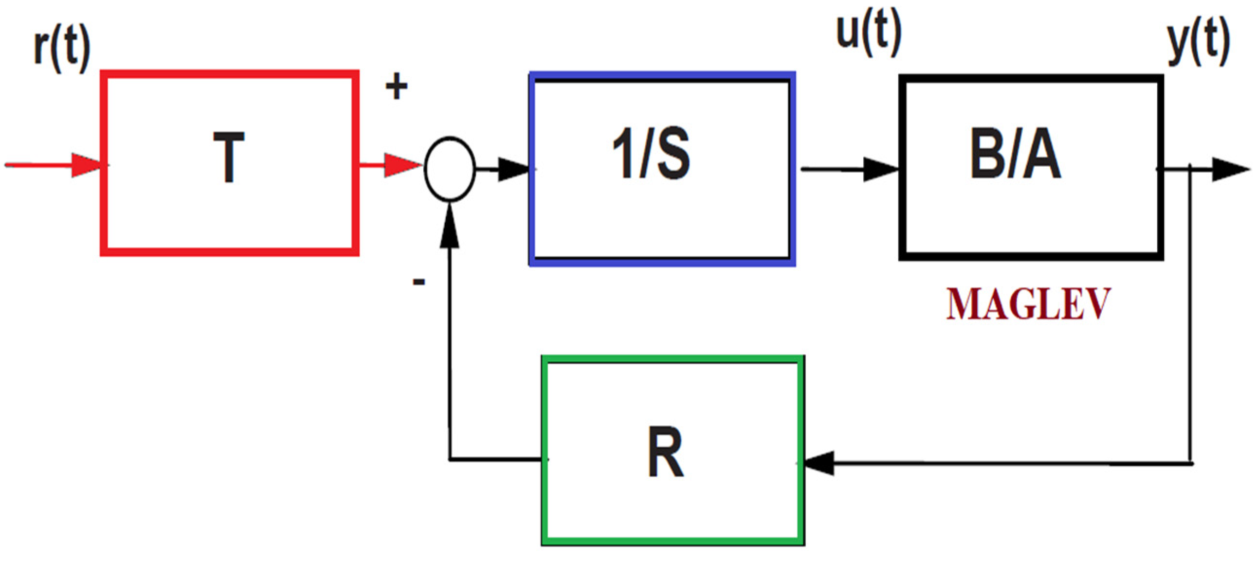
3.1. RST Controller Design

The RST control algorithm was used with the MAGLEV system (Figure 9) [15,19]:

$$S\left(q^{-1}\right)u\left(k\right)+R\left(q^{-1}\right)y\left(k\right)=T\left(q^{-1}\right)y^{*}\left(k\right)$$

(12)

where y(k) = process output, u(k) = algorithm output, and y*(k) = trajectory or filtered set point. The corresponding parameters are:

$$S\left(q^{-1}\right)=S_0+S_1{q}^{-1}+\cdots +S_{nS}{q}^{-nS}$$

(13)

$$R\left(q^{-1}\right)=r_0+r_1{q}^{-1}+\cdots +r_{nR}{q}^{-nR}$$

(14)

$$T\left(q^{-1}\right)=t_0+t_1{q}^{-1}+\cdots +t_{nT}{q}^{-nT}$$

(15)

The RST controller with a closed-loop system is shown in Figure 9.

The control law in (12) can be redesigned as shown below:

$$u\left(k\right)=\frac{1}{{\mathrm{s}}_0}\left[-R{\displaystyle \sum }_{i=1}^{n_S}{S}_i\mathrm{u}\left(\mathrm{k}-\mathrm{i}\right)-{\displaystyle \sum }_{i=0}^{n_R}{r}_i\mathrm{y}\left(\mathrm{k}-\mathrm{i}\right)+{\displaystyle \sum }_{i=0}^{n_T}{t}_i{\mathrm{y}}^{*}\left(\mathrm{k}-\mathrm{i}\right)\right]$$

(16)

$n_S , n_R , and n_T$ represent the respective polynomial degrees as well as the memory dimension for the algorithm’s software implementation. For example, if $n_R=2$, three memory places should be saved for the process’s output: $y\left(k\right), y\left(k-1\right), y\left(k-2\right).$ The same method applies to y*(k) and u(k), respectively.

One must be interested in the control method and, finally, the trajectory model generator for practical implementation. One cycle of the continuous monitoring procedure includes the following steps: acquisition of the process’s inputs; computation of the trajectory (if necessary); computation of the control law; transmission of the controls to the actuators; graphical representation of the process’s evolution; and memory update of the algorithms for the next iteration.

For example, if we have$n_S=n_R=n_T=2,$ and without trajectory generator (y*(k) = r(k)), the control law computation is as the following:

$$u\left(k\right)=\frac{1}{{\mathrm{s}}_0}\left(-S_1\mathrm{u}\left(\mathrm{k}-1\right)-r_0\mathrm{y}\left(\mathrm{k}\right)-r_1\mathrm{y}\left(\mathrm{k}-1\right)+t_0{\mathrm{y}}^{*}\left(\mathrm{k}\right)+t_1{\mathrm{y}}^{*}\left(\mathrm{k}-1\right)\right)$$

(17)

and (11) gives the algorithm’s memory actualization for the next iteration:

$$u\left(k-1\right)=u\left(k\right); y\left(k-1\right)=y\left(k\right); y^{*} \left(k-1\right)=y^{*} \left(k \right);$$

(18)

3.2. RST Controller Parameters Calculation

In this case, we used a pole placement procedure from the WinREG platform to figure out three RST algorithms. Through a second-order system, all systems were forced to have the same nominal performance, which is defined by the dynamics ${\omega }_0=7.5, \xi =0.8$ tracking performances, and disturbance rejection performances, respectively, while keeping the same sampling period as for the identification, $T_s=0.1$. All of these algorithms are only in charge of the process in their own zones.

$$\begin{array}{l}{R}_1\left(q^{-1}\right)=264.592-122.897 q^{-1}-6.19376 q^{-2}\\ S_1\left(q^{-1}\right)=1-0.98119 q^{-1}\\ T_1\left(q^{-1}\right)=135.5013\end{array}$$

$$\begin{array}{l}{R}_2\left(q^{-1}\right)=41.5417-21.46276 q^{-1}-0.60777 q^{-2}\\ S_2\left(q^{-1}\right)=1-0.96911 q^{-1}\\ T_2\left(q^{-1}\right)=20.686802\end{array}$$

$$\begin{array}{l}{R}_3\left(q^{-1}\right)=29.29215-15.25463 q^{-1}-0.56314 q^{-2}\\ S_3\left(q^{-1}\right)=1-0.94766 q^{-1}\\ T_3\left(q^{-1}\right)=14.600067\end{array}$$

3.3. Adaptive Supervisor and Switching

When the plant parameter vector switches rapidly (or discontinuously) between two values, p1 and p2, the adaptive method must be able to detect the change and switch to the appropriate controller to avoid catastrophic failure. The use of multiple (fixed) models permits the rapid selection of a fixed controller from a set of controllers, which can also be considered adaptive [22].

The following are some of the important questions that have to be addressed when multiple models are used for adaptive control:

(1)

When is it appropriate to make the transfer from one model to another? We need to decide which model to use;

(2)

When is a switching scheme stable? Will switching stop after a finite time? Will the switching scheme improve performance?

The switching criterion (or switching rule), which provides the answer to question (1), plays an important role in system design. Various performance indices can be chosen based on the estimation error to determine which of the models best fits the plant at any given time and should thus be used to regulate it. These may assume the following forms for continuous-time systems and their discrete-time counterparts.

The main method of switching depends on two main criteria, as shown in Figure 10. The first one is the set point because our multi-models depend on the level of the set point or zones, and the second one is the error, but this works just when the set point or model is in the common zones between two models, where the error identifies which controller is suitable. Three different zones are identified in the preview sections: Z1 (0–40%), Z2 (30–70%), and Z3 (60–100%). If we consider the desired position between 0 and 100 percent, the common zones are between Z1 and Z2 (30–40%) and between Z2 and Z3 (60–70%) [17].

4. Real-Time Implementation and Results

In this section, the experimental results for the proposed multi-controller and multi-model approaches with the MAGLEV system are presented. The local-platform system is proposed, as shown in Figure 11. LabVIEW was used to implement the real-time part with NI USB-6008 12-bit as the data acquisition. The MAGLEV system hardware also contains a Hall effect 49E sensor, electromagnetic coils, filters (hardware), a Dc Driver, and a real-time operating environment.

As an experiment, Case 1 was imposed, and the model M2 was the model of the system. Therefore, the controller of M2 in the multi-control approach was C2 $\left({\mathit{R}}_{\mathbf{2}},{\mathit{S}}_{\mathbf{2}},{\mathit{T}}_{\mathbf{2}}\right)$ but the system was forced to choose controller C1 as a test to see the response and performance of the Maglev system. Figure 12 depicts the response and performance of Case 1; slow rise time, high overshoot, high settling time, and weak rejecting the disturbances.

In the same way, considering the M2 as the main model of the system (Case 2), the process was repeated, but this time with $\left({\mathit{R}}_3,{\mathit{S}}_3,{\mathit{T}}_3\right)$ as the controller. The result was also not good, with slow rise time, higher overshoot, higher settling time, and weak ability to reject the disturbances, as shown in Figure 13.

Figure 14 depicts the effect of multi-model and multi-control on the MAGLEV response; the three zones show good and strong performances as overshoot, rise time, settling time, and rejection of the disturbances for all zones.

Table 1. Shows a comparison of the proposed solution (multi-model and multi-controller) (Zone 2 as a case study) versus a single controller (C1 with M2 and C3 with M2).

Controller Types	Overshoot	Settling Time	Rise Time	Disturbances
${\mathrm{RST}}_1\mathrm{with}\mathrm{M}2$	8.33%	1.1	0.36	Not good
${\mathrm{RST}}_3\mathrm{with}\mathrm{M}2$	16.4%	1.4	0.373	Not good
$\mathrm{Multi}\left(\mathrm{Model},\mathrm{Controller}\right)$ $\left(\mathrm{propused}\mathrm{solution}\right)$	1.1%	0.81	0.312	Good

shows a comprehensive comparison using the basic criteria.

* Figure 12, Figure 13 and Figure 14 represent (amplitude in volts and time in seconds).

The proposed real-time platform presents an economical solution that is not expensive (hardware and software) and more stable (hardware and software from National Instruments Company [23]) compared with our previous paper [13], which used elements from different companies. For example, the DC Driver and filters were created from cheap and basic components (resistors, capacitors, transistors, etc.).

The test of switching showed in Figure 15 that this method is stable. We can see that in both tests, there are either no shocks or low bumps in how the control evolves. As shown in

Table 2. Switching test in closed loop for all the zones.

Controller Types	Overshoot	Settling Time	Rise Time	Oscillations
$\mathrm{Switching}\mathrm{from}\mathrm{Z}1\mathrm{to}\mathrm{Z}2$	7.78%	0.94	0.32	Very small
$\mathrm{Switching}\mathrm{from}\mathrm{Z}2\mathrm{to}\mathrm{Z}3$	1.1%	0.81	0.312	No

, all of the parameters (overshoot, settling time, rise time, and shocks test) are excellent and proof that each model/identified process, in a closed loop, is stable. If there were more (4 or 5) models or algorithms, the little oscillations could be stopped.

The last comparison is between the results obtained in our previous paper [13] under the title (design of PID controller for nonlinear magnetic levitation system using fuzzy-tuning approach) (Figure 16) and the method in this paper. The result, shown in

Table 3. Comparison between the proposed solution (multi-model and multi-controller) with the results obtained in our previous paper [13] under the title (design of PID controller for nonlinear magnetic levitation system using fuzzy-tuning approach).

Controller Types	Overshoot	Settling Time	Rise Time	Disturbances
$\mathrm{Fuzzy}-\mathrm{PID}$	5.72%	0.85	0.68	Good
$\mathrm{Multi}\left(\mathrm{Model},\mathrm{Controller}\right)$ $\mathrm{with}\mathrm{RST}$ $\left(\mathrm{propused}\mathrm{solution}\right)$	1.1%	0.81	0.312	Good

, also shows that this method is better than (fuzzy-PID single controller) in overshoot, setting time rise time, and rejecting the disturbances.

5. Conclusions

The following findings can be drawn from the research:

• This paper deals with a magnetic-levitation (maglev) system. Real-time experimentation and simulations both confirmed the effectiveness of the maglev transportation system’s control strategy by using multi-model and multi-control approaches;
• The maglev system is nonlinear and very sensitive to disturbances, which is why the set point is divided into three zones to obtain three models;
• The three models were computed using the least-squares identification approach and the generation of pseudo-random signals (PRBS). LabVIEW and WinPIM were utilized in real-time to locate all models;
• The method’s applicability was demonstrated by utilizing a real-time structure with an RST control mechanism, and all parameters of the RST controller were computed by using the WinREG platform;
• Supervisor switching was implemented with two main criteria. The first one is the set point, and the second one is the level of the error;
• On the LabVIEW platform, experimental results are tested by conducting regulation and tracking experiments. The results of the experiments show that this method is very good, with strong response and stability. Smooth and exponential convergence of system variables to their desired levels with three zones;
• The experimental results also showed that the multi-zone model with multi-controller approaches is better with rising time, overshoot, settling time, rejecting the disturbances, and total response;
• The proposed real-time-platform presents an economical solution, not expensive (hardware and software), and more stable when compared with our previous paper [13];
• The obtained results sustain proposed solutions and suggest future steps, such as robustness conditions designed for bumpless switching in multiple model control structures [24];

References

1. Lee, H.W.; Kim, K.C.; Lee, J. Review of maglev train technologies. IEEE Trans. Magn. 2006, 42, 1917–1925. [Google Scholar]
2. Kumar, P.; Malik, S.; Toyserkani, E.; Khamesee, M.B. Development of an Electromagnetic Micromanipulator Levitation System for Metal Additive Manufacturing Applications. Micromachines 2022, 13, 585. [Google Scholar] [CrossRef] [PubMed]
3. Wang, H.; Liu, B.; Ping, X.; An, Q. Path tracking control for autonomous vehicles based on an improved MPC. IEEE Access 2019, 7, 161064–161073. [Google Scholar] [CrossRef]
4. Zhou, R.; Yan, M.; Sun, F.; Jin, J.; Li, Q.; Xu, F.; Zhang, M.; Zhang, X.; Nakano, K. Experimental validations of a magnetic energy-harvesting suspension and its potential application for self-powered sensing. Energy 2022, 239, 122205. [Google Scholar] [CrossRef]
5. Yan, L. Development and Application of the Maglev Transportation System. IEEE Trans. Appl. Supercond. 2008, 18, 92–99. [Google Scholar]
6. Xu, T.; Yu, J.; Yan, X.; Choi, H.; Zhang, L. Magnetic Actuation Based Motion Control for Microrobots: An Overview. Micromachines 2015, 6, 1346–1364. [Google Scholar] [CrossRef]
7. Xu, F.; Zhang, K.; Xu, X. Development of Magnetically Levitated Rotary Table for Repetitive Trajectory Tracking. Sensors 2022, 22, 4270. [Google Scholar] [CrossRef] [PubMed]
8. Mourad, A.; Youcef, Z. Adaptive Sliding Mode Control Improved by Fuzzy-PI Controller: Applied to Magnetic Levitation System. Eng. Proc. 2022, 14, 14. [Google Scholar] [CrossRef]
9. Al-Muthairi, N.; Zribi, M. Sliding mode control of a magnetic levitation system. Math. Probl. Eng. 2004, 2004, 93–107. [Google Scholar] [CrossRef]
10. Zhou, D.; Zhang, T.; Wang, L.; Li, J. Nonlinear Electromagnetic Force Model and Its Application to Magnetic Levitation Control System. In Proceedings of the 2022 8th International Conference on Control, Automation and Robotics (ICCAR), Xiamen, China, 8–10 April 2022; pp. 203–208. [Google Scholar] [CrossRef]
11. Boonsatit, N.; Pukdeboon, C. Adaptive fast terminal sliding mode control of magnetic levitation system. J. Control Autom. Electr. Syst. 2016, 27, 359–367. [Google Scholar] [CrossRef]
12. Ismail, L.S.; Petrescu, C.; Lupu, C.; Luu, D.L. Design of Optimal PID Controller for Magnetic Levitation System Using Linear Quadratic Regulator Approach. In Proceedings of the 2020 International Symposium on Fundamentals of Electrical Engineering (ISFEE), Bucharest, Romania, 5–7 November 2020; pp. 1–6. [Google Scholar] [CrossRef]
13. Ismail, L.S.; Lupu, C.; Alshareefi, H.; Luu, D.L. Design of PID controller for nonlinear Maglev system using Fuzzy-Tuning approach. U.P.B. Sci. Bull. Ser. C 2022, 84, 45–62. [Google Scholar]
14. Wong, T. Design of a magnetic levitation system—An undergraduate project. IEEE Trans. Educ. 1986, E-29, 196–200. [Google Scholar]
15. Landau, I.D.; Zito, G. Digital Control Systems; Springer: London, UK, 2006. [Google Scholar]
16. Fang, H.; Dianat, S.; Mestha, L.K.; Radomski, A. Developing a linear model of RF power generators with pseudo random binary signals (PRBS). In Proceedings of the 2014 14th International Conference on Control, Automation and Systems (ICCAS 2014), Gyeonggi-do, Korea, 22–25 October 2014; pp. 1158–1162. [Google Scholar] [CrossRef]
17. Lupu, C.; Popescu, D.; Ciubotaru, B.; Petrescu, C.; Florea, G. Switching solution for multiple-model control systems. In Proceedings of the 14th Mediterranean Conference on Control Autom, Ancona, Italy, 28–30 June 2006. [Google Scholar]
18. Liu, S.; Dong, R.; Chen, X. Application of the Main Steam Temperature Control Based on Sliding Multi-Level Multi-Model Predictive Control. In Proceedings of the 2017 International Conference on Computer Systems, Electronics and Control (ICCSEC), Dalian, China, 25–27 December 2017; pp. 875–880. [Google Scholar] [CrossRef]
19. Popescu, D.; Stefanoiu, D.; Lupu, C.; Ciubotaru, B.; Petrescu, C.; Dimon, C. Automatica Industrial; Agir: Bucharest, Romania, 2006. [Google Scholar]
20. Lehouche, H.; Guéguen, H.; Mendil, B. Set-point supervisory control methodology for a nonlinear continuous stirred tank reactor process. Arab. J. Sci. Eng. 2012, 37, 831–849. [Google Scholar] [CrossRef]
21. Balakrishnan, J. Control System Design Using Multiple Models, Switching and Tuning. Ph.D. Dissertation, University of Yale, New Haven, CT, USA, 1996. [Google Scholar]
22. Narendra, K.S.; Driollet, O.A.; Feiler, M.; George, K. Adaptive control using multiple models, switching and tuning. Int. J. Adapt. Control Signal Process. 2003, 17, 87–102. [Google Scholar] [CrossRef]
23. National Instruments Corporation. Available online: https://www.ni.com (accessed on 24 July 2022).
24. Lupu, C.; Nasture, A.M.; Ismail, L.S.; Lupu, M. Safety Concerning for Algorithms Switching in Multiple Model Control Structures. In Proceedings of the 2020 24th International Conference on System Theory, Control and Computing (ICSTCC), Sinaia, Romania, 8–10 October 2020. [Google Scholar]
Figure 1. Magnetic Levitation System Block Diagram.
Asi 05 00093 g001
Figure 2. Nonlinear multiple zone diagram of the process.
Asi 05 00093 g002
Figure 3. System Identification diagram of the process.
Asi 05 00093 g003
Figure 4. PRBS generation in LabVIEW.
Asi 05 00093 g004
Figure 5. Input and output signals for Model 1.
Asi 05 00093 g005
Figure 6. Input and output signals for Model 2.
Asi 05 00093 g006
Figure 7. Input and output signals for Model 3.
Asi 05 00093 g007
Figure 8. Structure of the system with supervisory control architecture.
Asi 05 00093 g008
Figure 9. RST algorithm.
Asi 05 00093 g009
Figure 10. Adaptive Supervisor and switching.
Asi 05 00093 g010
Figure 11. The magnetic levitation system platform.
Asi 05 00093 g011
Figure 12. Performances for Z2 operating point with ( R 1 , S 1 , T 1 )   algorithm *.
Asi 05 00093 g012
Figure 13. Performances for Z2 operating point with ( R 3 , S 3 , T 3 )   algorithm *.
Asi 05 00093 g013
Figure 14. Multi-model controller real-time with Maglev system application and performances for Z2 operating point with ( R 2 , S 2 , T 2 )   algorithm *.
Asi 05 00093 g014
Figure 15. Switching test (Z2 to Z3).
Asi 05 00093 g015
Figure 16. The response of PID controller using fuzzy-tuning approach [13].
Asi 05 00093 g016