Article

Analysis of GNSS Data for Earthquake Precursor Studies Using IONOLAB-TEC in the Himalayan Region

1
Indian Institute of Remote Sensing, ISRO, Dehradun 248001, Uttarakhand, India
2
Birla Institute of Applied Sciences, Nainital 23616, Uttarakhand, India
*
Author to whom correspondence should be addressed.
Quaternary 2023, 6(2), 27; https://doi.org/10.3390/quat6020027
Submission received: 1 December 2022 / Revised: 14 February 2023 / Accepted: 11 April 2023 / Published: 19 April 2023
(This article belongs to the Collection Feature Papers in Quaternary Research)

Abstract

:
Earthquake precursors are the indicators that appear before an earthquake. The release of radon gas, ionospheric disturbances, anomalous animal behavior, and so on are examples of seismic and aseismic events. Ionospheric perturbations can be proved to be a reliable method in earthquake prediction. The GNSS data detect changes in the ionosphere through the time lag of the transmitted GPS signals recorded at the Earth-based receivers. A negative TEC anomaly is caused by the stress released from the rocks before the earthquake, which elevates positive ions or p-holes in the atmosphere and decreases the ions in the ionosphere. A positive TEC anomaly follows this because of the increase in ions in the ionosphere. The ionospheric disruption in the Himalayan region is examined before five random earthquakes. For this, data from 15 separate GNSS stations are investigated using IONOLAB-TEC. A promising total electron content (TEC) data estimate with a temporal resolution of 30 s was analyzed. The results of the TEC data analysis depict the anomaly a month before the five earthquakes, followed by the later perturbation in the earthquake preparation zone. TEC anomalies are enhanced more by the uniform spatial distribution of GNSS stations in the epicentral region than by randomly distributed stations. The results of IONOLAB-TEC and the widely used GPS-TEC software were compared. Owing to its temporal resolution, IONOLAB-TEC has edge over the GPS-TEC software in that it can identify even the slightest negative anomalies before an earthquake.

1. Introduction

An earthquake precursor is the anomalous behavior observed before an earthquake in the form of either radon gas emission, ionospheric disturbances, or anomalous animal behavior. Much literature has studied animal behavior changes before a major earthquake. The works of [1,2,3,4,5,6,7,8,9] observed the changes in animal behavior vis-à-vis geomagnetic and ionospheric perturbations. It has been suggested that ground vibrations, humidity, temperature, atmospheric pressure changes, electromagnetic field (EMF) emissions, and gas/chemical emissions prior to earthquakes could be sensed by animals through a seismic escape behavioral system [2,3,4,5,6,7]. Prior to an earthquake, the build-up of stress causes changes in rock pressures and fluid convective flows [10]. The fault displacement of rock mass under that tectonic stress opens various pathways to the surface and unusual quantities of radon emission through fractures [10,11]. The stress released from the rocks perturbs their peroxy bonds, and their breakup leads to the release of positively charged particles, known as p-holes. These p-holes then reach the Earth’s surface and migrate toward the atmosphere. They drag electrons downward as soon as they reach the lower ionosphere. This alters the ionosphere’s vertical distribution of ions and electrons, and the satellite signals are impacted by these changes in the ionosphere. The significance of ionospheric perturbations as an earthquake precursor is addressed in the literature [12,13,14,15,16,17,18,19]. Global navigation satellite system (GNSS) for ionospheric precursor studies has also been used in the high seismic regions of the world, such as Chile and Japan. The study of the 2011 Japan earthquake of Mw 9.0 by Yao [20] investigates pre-earthquake ionospheric anomalies and their temporal and spatial characteristics using data from GNSS and ionosonde stations near the epicenter. It depicts that the ionospheric anomaly was detected three days before the earthquake, considered a promising anomaly for the impending earthquake. The work of Báez et al. [21] presented the state-of-the-art methods and products of the Chilean GNSS network, with a focus on the applications to real-time detection of coseismic deformation and rapid response capabilities for moderate-to-large earthquakes. The spatial density of the GNSS networks is also increasing for their use in early warning systems for earthquakes and tsunamis [21]. The successful implementation of IONOLAB-TEC in the earthquake precursor studies of various earthquakes around the globe is addressed in the literature [22,23]. Inyurt et al. [22] utilized IONOLAB-TEC along with GIM-TEC to acquire TEC values for respective stations. They observed numerous positive TEC anomalies due to solar and geomagnetic activities. In order to investigate whether the anomalies before, on the day of, and after the earthquake was caused by the earthquake, the (Kp⋅10), Dst, and F10.7 cm indices, which provide information on the geomagnetic and solar activity for the days, were examined, in which anomalies were detected [22]. Differentiating it from the anomalies of the earthquake became a difficult task. Therefore, they suggested a multidisciplinary study to identify ionospheric changes as an earthquake precursor under disturbed space weather conditions [22]. Contadaet al. al. [23] analyzed the TEC variations over the Mediterranean through IONOLAB-TEC using discrete Fourier analysis during the earthquake of 12 October 2013, which occurred west of Crete, Greece. They observed that the TEC variations that ensued might be due to the earthquake. However, the lithosphere–atmosphere–ionosphere coupling (LAIC) mechanism through acoustic or gravity waves could explain the accurate phenomenon behind the TEC variations.
The analysis of GNSS data using IONOLAB-TEC was chosen to study the five earthquakes in the Himalayan region. The first objective of this study is to prepare the earthquake preparation zones of five earthquakes and to determine three GNSS base stations for each earthquake within the preparation zone. The second objective is to acquire data using IONOLAB-TEC for two months. The third objective is to calculate the upper and lower bound TEC values using the equations given by [24]. The TEC values outside the limits will be considered anomalies and, therefore, considered as a precursor of the earthquake in that region.

2. Study Area

The Himalayan belt, created by the collision of the Indian and Eurasian plates around 50 million years ago, is one of the most earthquake-prone regions. It broadly consists of four major regions. The Sub-Himalaya and Lesser Himalaya abruptly rise above the Ganga valley, the Lesser Himalaya gradually gains altitude, the Lesser Himalaya and the High Himalayan range are connected by a steep slope, and the High Himalayan range is characterized by a consistent elevation of around 5 km. The faults associated with them are the hosts of devastating earthquakes. The earthquakes chosen for the analysis of TEC variations are 2015 Nepal (Mw 7.3), 2016 Imphal (Mw 6.7), 2020 Myanmar (Mw 5.9), 2020 Nepal (Mw 4.9), and 2020 Manipur (Mw 5.2) (Table 1). These three regions have complex lithology and geological structures. Owing to the continuous movement of the Himalaya, these regions have numerous faults, fractures, and lineaments with sheared, weak, and metamorphosed rocks that host numerous earthquakes of varying magnitudes. The Central Himalayan crystalline rocks in Nepal are laced with dense faults and fractures. Because of this, Nepal experiences devastating earthquakes of considerable magnitude and shallow depth. With its original basin topography of ridges and furrows, Manipur (India) is a part of the vast geosynclines. Being close to the Indo-Myanmar arc, Manipur frequently experiences earthquakes of diverse magnitudes. Myanmar is located at the confluence of the Alpine-Himalayan Orogenic Belt and the Indonesian Island Arc System [25]. In northern Myanmar, the orogenic belt is bent around the Eastern Himalayan Syntaxis in a north-south direction. It passes southward through the Indo-Myanmar Ranges [25,26,27,28] into the Andaman and Nicobar Islands, Sumatra, and Indonesia’s Sunda and Banda arcs [25]. The mountain ranges in northern Myanmar are clear evidence of the collision of the Indian and Eurasian plates, leading to frequent earthquakes in the region. Figure 1 shows the DEM image of parts of Central and Eastern Himalaya displaying five earthquake epicenters along with the significant seismogenic thrusts of the Himalayas, i.e., Himalayan Frontal Fault (MFT), Main Boundary Thrust (MBT), and Main Central Thrust (MCT), with MCT being the main thrust region for the earthquakes of higher magnitude.

3. Data and Method

3.1. Data Used

The base station located within the epicenter’s earthquake preparation zone provided the data for the study of the ionospheric perturbations. The National Oceanic and Atmospheric Administration (NOAA) provides information for negating geomagnetic disruption. Geomagnetic activity is classified using the NOAA classification. The day is geomagnetically stormy if the Ap index consists of values between 29 and 100. A minor storm is predicted if Ap index values are between 29 and 50. A significant storm is determined when 50 ≤ Ap < 100, and a severe storm is predicted when Ap ≥ 100.

3.2. IONOLAB-TEC

IONOLAB-TEC is the executable software that employs the Reg-est algorithm. The regularized-estimation (Reg-Est) algorithm is a new alternative for the estimation of robust TEC values by combining GPS/GNSS measurements of 30 s resolution obtained from the satellites above the 10° elevation limit, ‘in press’ [29]. This software is successfully used in various works in the literature for various earthquakes. The M 7.4 earthquake in Mexico on 23 June 2020 was investigated using IONOLAB-TEC. This paper observed the air temperature, total electron content, and air relative humidity as precursors of earthquakes. The atmospheric air temperature and outgoing longwave radiation (OLR) indicate significant positive anomalies above the epicenter of the earthquake prior to the major earthquake occurrence [30]. The atmospheric relative humidity shows a significant negative anomaly above the epicenter of the earthquake prior to the major earthquake occurrence [30]. These TEC perturbations before the earthquake during quiet geomagnetic storms and inactive solar flux conditions were locally observed and can be considered the precursor of an impending earthquake. Another study has been carried out for the M 6.3 Abruzzo earthquake of 6 April 2009. The results showed that the TEC variations occurred randomly over several hundred kilometers from the earthquake [31]. The high-frequency oscillations indicated the location of the earthquake but with limited accuracy. This algorithm is also significant because it is a key substitute for monitoring ionospheric irregularities and sudden disturbances. Receiver Independent Exchange (RINEX) data, Differential Code Bias (DCB) data, Standard Product (SP3) data, and Ionosphere Map Exchange (IONEX) data were used to determine the slant TEC (STEC) and vertical TEC (VTEC) values. The Reg-Est algorithm derives TEC values by combining the VTEC for each satellite in the least square sense while using a weighting function to minimize the multipath effects [29]. The method used for the computation of STEC, VTEC, and the mapping function is provided below. STEC is converted to VTEC using the mapping function M. The instrumental biases here are in time units.
S T E C u m n = 1 A f 1 2 f 2 2 f 1 2 f 2 2 [ P 4 , u m n + c D C B m + D C B u ]
V T E C u m n = S T E C u m ( n ) / M ( ɛ m n )
M ɛ m n = 1 R c o s ɛ m ( n ) R + h 2 1 2
where,
P4 = geometry free linear combination of pseudorange values (P4 = P2 − P1)
A = constant = 40.3 m3/s2
DCBm = frequency-dependent satellite instrumental bias
DCBu = frequency-dependent receiver instrumental bias
M = mapping function
ɛ = satellite elevation angle
m = satellite
u = receiver
n = time

3.3. Method of Analysis of TEC Data

The analysis of ionospheric perturbations from five earthquakes in the Himalayas uses three IGS base stations for each earthquake to determine the ionospheric perturbations (Table 2). The strain radius was calculated based on Dobrovolsky’s equation: Strain radius (p) = 100.43M km (where M = magnitude) [32]. The work is carried out by acquiring two months’ worth of data for 15 IGS stations. It has been observed that the ionosphere’s variability increases locally within the earthquake preparation zone a few days before the seismic event [24]. This fact has been considered in the present study to estimate the variation in TEC in the ionosphere [24]. It varies from 1337 km for the Mw 7.3 Nepal 2015 earthquake to 127.94 km for the Mw 4.9 Nepal 2020 earthquake. Table 2 shows the distances between the epicenters of these earthquakes and the GNSS and receiver stations used in this analysis.
To identify seismo-ionospheric signals, we examined the behavior of VTEC for 120 running days using statistical methods [14,24,31]. The median of 15 running days was computed to construct the upper and lower bounds [24]:
U p p e r   B o u n d = X + 1.34 σ
L o w e r   B o u n d = X 1.34 σ
where X is the median and σ is the standard deviation [24]. VTEC values above the upper bound or below the lower bound are considered an anomaly.

4. Results

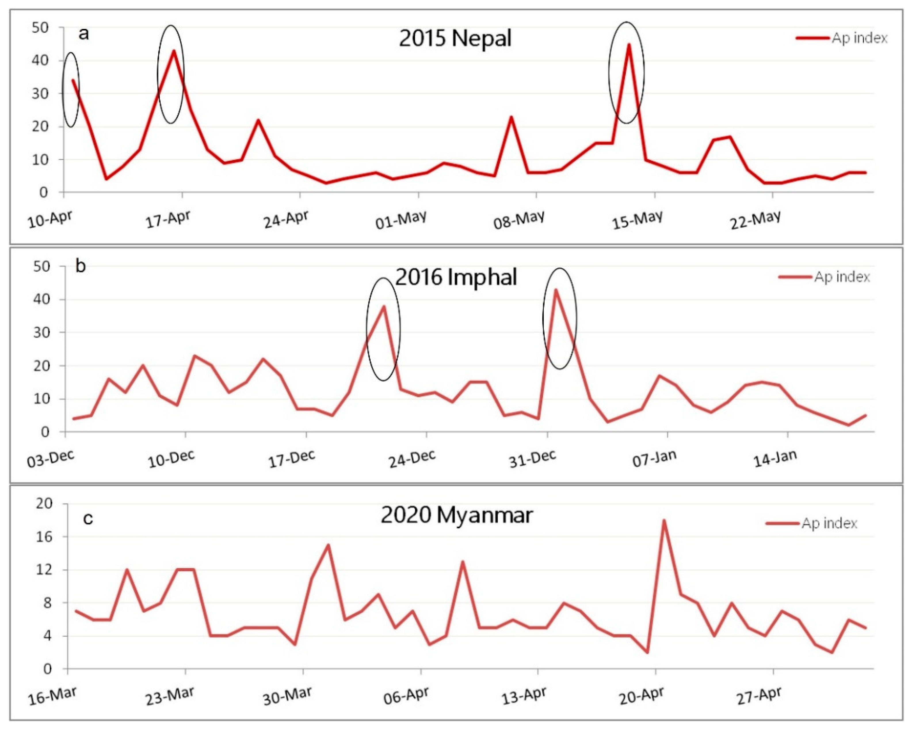
4.1. 2015 Nepal Earthquake

The Mw 7.3 Nepal earthquake occurred on 12 May 2015 at 07:05:19 UTC. GNSS data from the base stations SYBC, NAST, and CHLM were prepared between 26 March and 27 May 2015 to determine TEC variations between 10 April and 27 May 2015. Figure 2 depicts data from the CHLM station, located 86 km from the epicenter. The GNSS data processing revealed negative and positive anomalies (Table 3). One month before the occurrence, on 11 April, the first negative anomaly was observed. Additionally, a negative anomaly was observed on 11 May, the day before the earthquake. Then for seven days, from 19 May to 25 May, a consistent and significant negative anomaly was observed after the event. Likewise, on 14 April, the first positive anomaly was observed. On the day of the event, a positive anomaly was also observed, and the peak value was recorded at 08:02 UTC with a TEC value of 88.52 TECU. According to the geomagnetic data, there were light storms on 10 April and 16 April, and 13 May, with corresponding Ap indices of 34, 43, and 45, respectively (Figure 7). The geomagnetic activity was, therefore, responsible for the positive anomalies seen on these three days.

4.2. 2016 Imphal Earthquake

On 3 January 2016, at 23:05:22 UTC, there was an earthquake in Imphal measuring Mw 6.7. GNSS data from the IGS stations SYBC, RMJT, and RMTE from 18 November 2015 to 18 January 2016 were compiled to calculate TEC variations from 3 December 2015 to 18 January 2016. The data obtained from the station RMTE, located 745.08 km from the epicenter, are displayed in Figure 3. In Table 3, the anomalies discovered using GNSS data are listed. On 4 and 3 December, the first negative and positive anomalies, respectively, were noticed (one month before the event). A second positive anomaly was observed on 31 December at 8:54 UTC. The geomagnetic environment was calm, except for 21 December and 31 December 2015 (Figure 7). The Ap index observed was 38 and 43 respectively, contributing to the minor storm and high electron content. Thus, geomagnetic activity accounts for the positive anomalies recorded on these days. This anomaly is a true earthquake precursor because the negative anomaly was also detected on 31 December.

4.3. 2020 Myanmar Earthquake

The Mw 5.9 Myanmar earthquake occurred on 16 April 2020 at 11:45 UTC. From 1 March to 2 May 2020, GNSS data from IGS stations KALW, KLAY, and TEDM were prepared to derive TEC variations from 16 March to 2 May 2020. Figure 4 shows the data acquired from the station KLAY, which is 45.35 km from the epicenter. Table 3 shows negative and positive anomalies in the processed GNSS data. The first negative anomaly was observed on 22 March, 25 days before the event. The negative anomalies were also observed on the day of the event at 5:37:45 UTC. The first positive anomaly was observed on 21 March, 26 days before the event. Throughout the duration, the geomagnetic conditions were calm. No geomagnetic activity was observed in the acquired data (Figure 7).

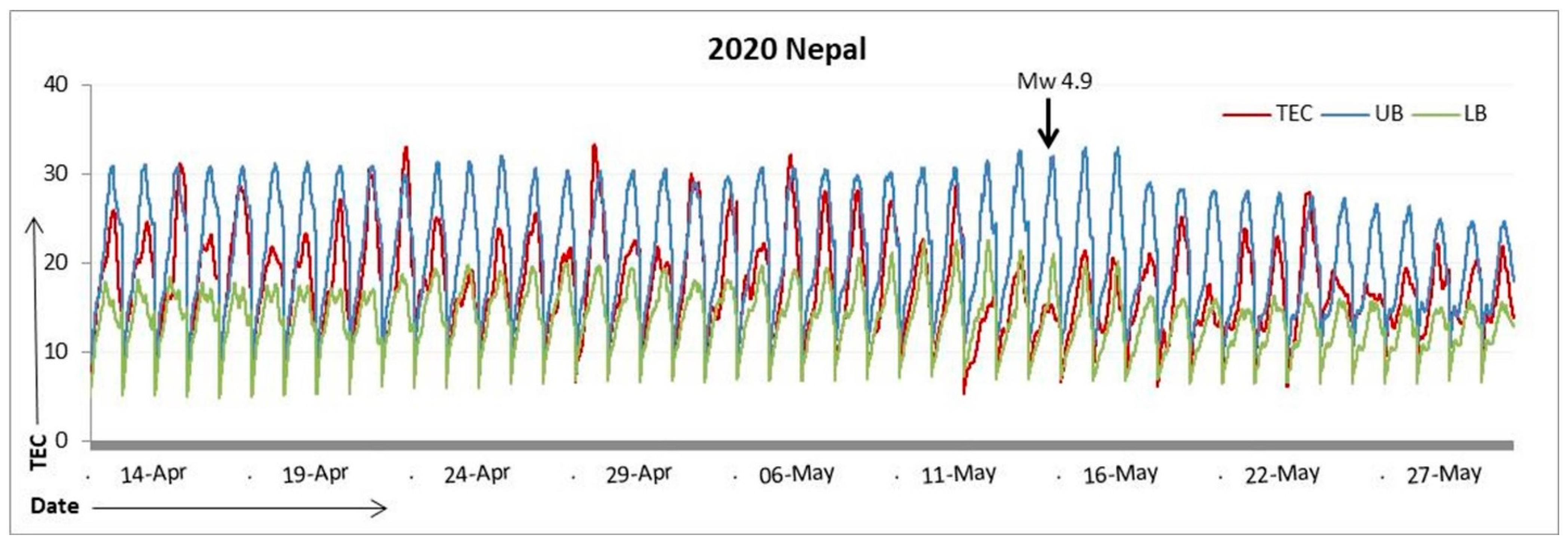
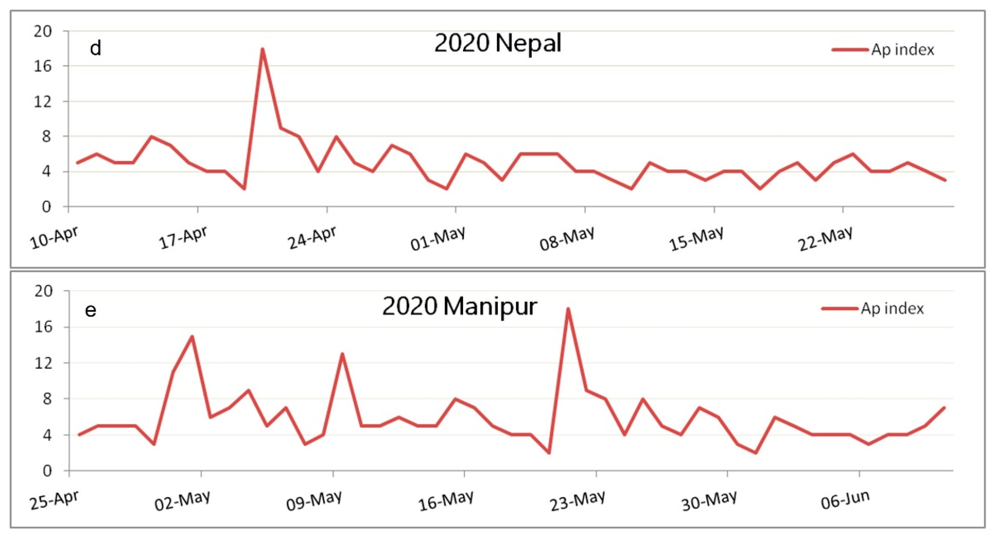
4.4. 2020 Nepal Earthquake

The Mw 4.9 Nepal earthquake occurred on 12 May 2020 at 18:08:38 UTC. From 26 March to 27 May 2020, GNSS data from IGS stations JIR2, KUGE, and SYBC were processed to derive TEC variations from 10 April to 27 May 2020. Figure 5 shows the data acquired from station JIR2, which is 13.41 km from the epicenter. The processed GNSS data revealed negative and positive anomalies, as shown in Table 3. The first negative anomaly was observed on 13 April, one month before the event. The first positive anomaly was observed on 13 April, a month before the earthquake. A continuous positive anomaly was observed for 19 – 20 April, 26 April, 29 April, and 1 May. Throughout the duration, the geomagnetic conditions were calm. No geomagnetic activity was observed in the acquired data (Figure 7).

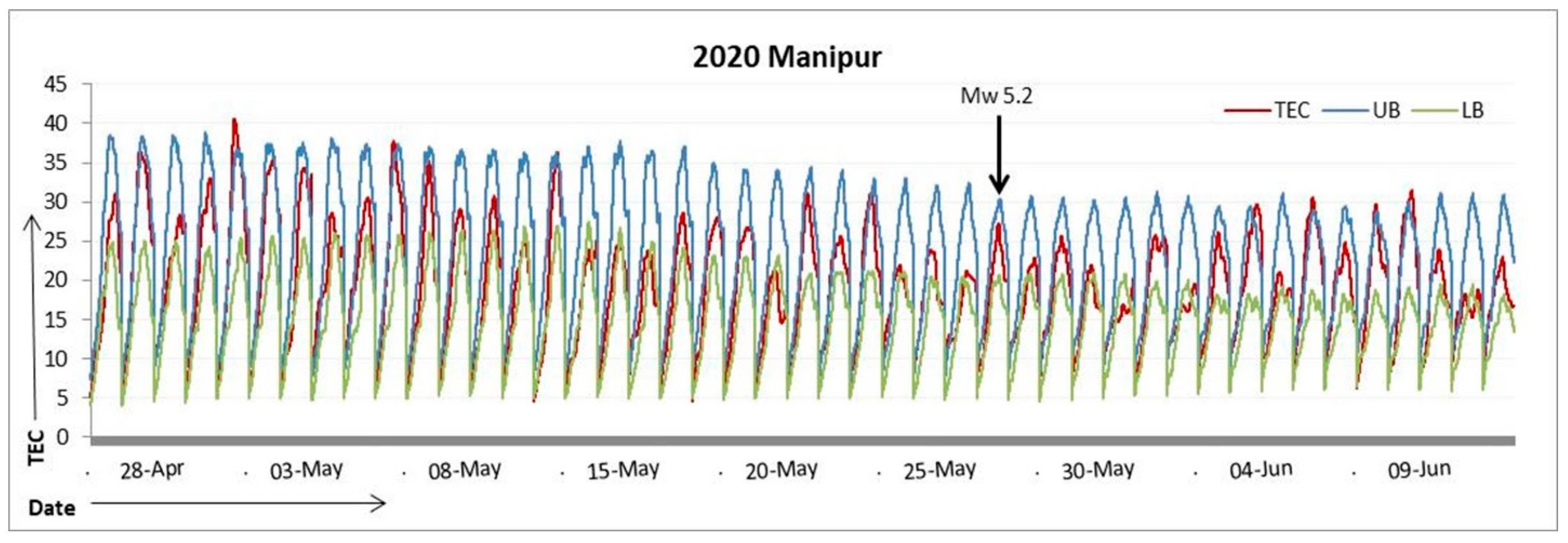
4.5. 2020 Manipur Earthquake

The Mw 5.2 Manipur earthquake, located at 24.391° N and 93.921° E, occurred on 25 May 2020, at 14:42:17 UTC. From 10 April to 10 June 2020, GNSS data from IGS stations KALW, KLAY, and TEDM were processed to derive TEC variations from 25 April to 10 June 2020. Figure 6 shows the data acquired from the station TEDM, 120.02 km from the epicenter. The processed GNSS data revealed negative and positive anomalies (Table 3). The first negative anomaly was observed on 25 April, one month before the event. The first positive anomaly was observed on 29 April and 30, 27, and 26 days before the earthquake (Figure 6). Throughout the duration, the geomagnetic conditions were calm. No geomagnetic activity was observed in the acquired data (Figure 7).

5. Discussion

5.1. Compatibility of IONOLAB-TEC

Given that IONOLAB-TEC has yet to be utilized in the Himalayan region, determining its accuracy and effectiveness was essential. Therefore, the two earlier earthquakes (2015 Nepal and 2016 Imphal) with their documented anomalies were chosen for this project. The data were then correlated with [19,24] for the earthquakes in 2015 in Nepal and 2016 in Imphal. The results showed that IONOLAB-TEC helped analyze earthquake precursors in the Himalayan region. This software’s higher temporal resolution detected more anomalies before and after the earthquake than with the [19,24] anomalies which have GPS -TEC software.

5.2. Accuracy of the Ionospheric Perturbation as an Earthquake Precursor

The extra-terrestrial phenomenon can also disrupt the ionospheric system. As a result, the precision of the outcomes produced by TEC values is related to the geomagnetic data. Before the 2015 Nepal earthquake (M7.3), significant negative anomalies were observed. No anomaly was observed near the 2016 Imphal earthquake. On the day of the earthquake in 2020 in Myanmar (Falam), a negative anomaly was detected. On the day of the event, at 5:13:30 UTC, a negative anomaly was observed in the 2020 Nepal earthquake. The observed anomalies were significant despite their small magnitude because the station was close to the epicenter. A positive anomaly was observed on the day of the earthquake in Manipur (Kakching) at around 04:53:30 UTC.
The ionospheric perturbation in the Imphal earthquake of 2016 has gained some validity in the precursor study. As stated, abnormalities of both a positive and negative nature were seen on 31 December 2015. A minor geomagnetic disturbance occurred on that day (Figure 7). A negative anomaly with a VTEC of 14.83 TECU was observed on that day at 03:07:00 UTC, while a positive anomaly with a VTEC of 53.4 TECU was observed at 08:49:00 UTC. Therefore, seismic disturbances were the only reason the TEC anomaly occurred.

5.3. TEC Variation with Respect to the Epicentral Distance

With various epicentral distances, slight variations were observed. Table 3 lists the various stations, the distances between the five epicenters, and the detected anomalies. Figure 8 depicts a graph of the TEC variation of the different earthquake stations. The SYBC station, closer to the epicenter (63.7 km), provides the highest TEC values for the 2015 Nepal earthquake. Continuous TEC variations after the quake were observed the most with the 2015 Nepal earthquake. All stations are close to the edge of the earthquake preparation zone for the Imphal earthquake of 2016. As a result, the difference in TEC values among the stations could be more noticeable. All three stations are located near to one another in the 2020 Myanmar earthquake. Consequently, TEC values were observed to be low. This indicates that a better station distribution is recommended to calculate the TEC variation. The JIR2 station’s value of TEC fluctuations for the 2020 Nepal earthquake is higher owing to its proximity to the epicenter. Owing to their proximity, all three stations provide similar TEC values for the 2020 Manipur earthquake. Compared with stations far from the epicenter, those closer to the epicenter exhibit higher intensities and more frequent anomalies.

6. Conclusions

To analyze ionospheric perturbations, the analysis of GNSS data using IONOLAB-TEC examines the TEC variation in the Himalayan region. The 30 s resolution provided by IONOLAB-TEC detects minor anomalies better than GPS-TEC. The analysis found that anomalies are detected one month before the earthquake, except for the 2020 Myanmar earthquake (Mw 5.9). The TEC anomalies are detected on the day of the earthquake, except for the 2016 Imphal earthquake (Mw 6.7). However, no regular patterns were observed in the TEC perturbations within these five earthquakes. The TEC perturbations were also observed after the event and were recorded to be highest in the 2015 Nepal earthquake. Higher magnitude earthquakes show more evidence of the TEC variation’s frequency. When a high-magnitude earthquake occurred, the TEC anomalies were noticed for extended periods. The earthquake’s depth also impacted the TEC value. For shallower earthquakes, larger values were reported. Better spatial distribution of the GNSS stations is a requirement for real-time monitoring. The clarity in the realm of earthquake prediction requires constant observation of real-time TEC data.

Author Contributions

Conceptualization, S.K.; methodology, S.K.; software, S.J. and U.J.; validation, S.K.; formal analysis, S.J.; investigation, S.K.; resources, S.K.; data curation, U.J. and S.J.; writing—original draft preparation, S.J.; writing—review and editing, S.K. and S.J.; visualization, S.J.; supervision, S.K.; project administration, S.K. All authors have read and agreed to the published version of the manuscript.

Funding

This work is part of the Post graduate diploma pilot project. Therefore, no external funding is involved.

Data Availability Statement

The TEC data has been acquired from the IONOLAB-TEC Software itself. The geomagnetic data has been acquired from NOAA website (https://www.ngdc.noaa.gov/stp/geomag/kp_ap.html, accessed on 13 October 2022). To prepare the study map, DEM images from USGS are used.

Acknowledgments

The authors express their gratitude to Chairman ISRO, Director IIRS ISRO Dehradun for their constant support and encouragement in carrying out this work smoothly. We also acknowledge the support from Feza Arikan, Umut Sezen, and the team of IONOLAB-TEC for answering all queries and updating the software. The authors are also grateful to the International GNSS Station (IGS), University NAVSTAR Consortium (UNAVCO), and National Oceanic and Atmospheric Administration (NOAA) for freely providing high-quality GNSS and geomagnetic data and to the USGS Earth Explorer for giving a platform to acquire high-quality free satellite data. The authors would like to dedicate this work to the late P.K. Champati Ray, whom we lost to COVID-19. His unrivaled support and vision helped us put the piece together.

Conflicts of Interest

The authors declare no conflict of interest.

References

  1. Tributsch, H. When the Snakes Awake: Animals and Earthquake Prediction. 1982. Available online: https://www.osti.gov/biblio/5345152 (accessed on 5 January 2023).
  2. Rikitake, T. The Science of Macro-Anomaly Precursory to an Earthquake; Kinmiraisha: Nagoya, Japan, 1998. [Google Scholar]
  3. Kirschvink, J.L. Earthquake Prediction by Animals: Evolution and Sensory Perception. Bull. Seismol. Soc. Am. 2000, 90, 312–323. [Google Scholar] [CrossRef]
  4. Bhargava, N.; Katiyar, V.K.; Sharma, M.L.; Pradhan, P. Earthquake Prediction through Animal Behavior: A Review. Indian J. Biomech. 2009, 78, 159–165. [Google Scholar]
  5. Cicerone, R.D.; Ebel, J.E.; Britton, J. A Systematic Compilation of Earthquake Precursors. Tectonophysics 2009, 476, 371–396. [Google Scholar] [CrossRef]
  6. Hayakawa, M. Possible Electromagnetic Effects on Abnormal Animal Behavior before an Earthquake. Animals 2013, 3, 19–32. [Google Scholar] [CrossRef] [PubMed]
  7. Lakshmi, K.R.; Nagesh, Y.; Krishna, M.V. Analysis on Predicting Earthquakes through an Abnormal Behavior of Animals. Int. J. Sci. Eng. Res. 2014, 5, 845–857. [Google Scholar]
  8. Woith, H.; Petersen, G.M.; Hainzl, S.; Dahm, T. Review: Can Animals Predict Earthquakes? Review: Can Animals Predict Earthquakes? Bull. Seismol. Soc. Am. 2018, 108, 1031–1045. [Google Scholar] [CrossRef]
  9. Panagopoulos, D.J.; Balmori, A.; Chrousos, G. On the Biophysical Mechanism of Sensing Upcoming Earthquakes by Animals. Sci. Total Environ. 2020, 717, 136989. [Google Scholar] [CrossRef]
  10. Ambrosino, F.; Thinová, L.; Briestenský, M.; Šebela, S.; Sabbarese, C. Detecting Time Series Anomalies Using Hybrid Methods Applied to Radon Signals Recorded in Caves for Possible Correlation with Earthquakes. Acta Geod. Geophys. 2020, 55, 405–420. [Google Scholar] [CrossRef]
  11. Anderson, O.L.; Grew, P.C. Stress Corrosion Theory of Crack Propagation with Applications to Geophysics. Rev. Geophys. 1977, 15, 77. [Google Scholar] [CrossRef]
  12. Freund, F. Conversion of Dissolved “Water” into Molecular Hydrogen and Peroxy Linkages. J. Non-Cryst. Solids 1985, 71, 195–202. [Google Scholar] [CrossRef]
  13. Pulinets, S. Ionospheric Precursors of Earthquakes; Recent Advances in Theory and Practical Applications. Terr. Atmos. Ocean. Sci. 2004, 15, 413. [Google Scholar] [CrossRef]
  14. Liu, J.Y.; Chuo, Y.J.; Shan, S.J.; Tsai, Y.B.; Chen, Y.I.; Pulinets, S.A.; Yu, S.B. Pre-Earthquake Ionospheric Anomalies Registered by Continuous GPS TEC Measurements. Ann. Geophys. 2004, 22, 1585–1593. [Google Scholar] [CrossRef]
  15. Stiros, S.C. The 8.5+ Magnitude, AD365 Earthquake in Crete: Coastal Uplift, Topography Changes, Archaeological and Historical Signature. Quat. Int. 2010, 216, 54–63. [Google Scholar] [CrossRef]
  16. Ouzounov, D.; Pulinets, S.; Romanov, A.; Romanov, A.; Tsybulya, K.; Davidenko, D.; Kafatos, M.; Taylor, P. Atmosphere-Ionosphere Response to the M9 Tohoku Earthquake Revealed by Multi-Instrument Space-Borne and Ground Observations: Preliminary Results. Earthq. Sci. 2011, 24, 557–564. [Google Scholar] [CrossRef]
  17. Heki, K. Ionospheric Electron Enhancement Preceding the 2011 Tohoku-Oki Earthquake. Geophys. Res. Lett. 2011, 38. [Google Scholar] [CrossRef]
  18. Sharma, M.L.; Lindholm, C. Earthquake Hazard Assessment for Dehradun, Uttarakhand, India, Including a Characteristic Earthquake Recurrence Model for the Himalaya Frontal Fault (HFF). Pure Appl. Geophys. 2011, 169, 1601–1617. [Google Scholar] [CrossRef]
  19. Sharma, G.; Champati ray, P.K.; Mohanty, S.; Kannaujiya, S. Ionospheric TEC Modelling for Earthquakes Precursors from GNSS Data. Quat. Int. 2017, 462, 65–74. [Google Scholar] [CrossRef]
  20. Yao, Y.; Chen, P.; Wu, H.; Zhang, S.; Peng, W. Analysis of Ionospheric Anomalies before the 2011 M W 9.0 Japan Earthquake. Chin. Sci. Bull. 2012, 57, 500–510. [Google Scholar] [CrossRef]
  21. Báez, J.C.; Leyton, F.; Troncoso, C.; del Campo, F.; Bevis, M.; Vigny, C.; Moreno, M.; Simons, M.; Kendrick, E.; Parra, H.; et al. The Chilean GNSS Network: Current Status and Progress toward Early Warning Applications. Seismol. Res. Lett. 2018, 89, 1546–1554. [Google Scholar] [CrossRef]
  22. Inyurt, S.; Peker, S.; Mekik, C. Monitoring Potential Ionospheric Changes Caused by the van Earthquake. Ann. Geophys. 2019, 37, 143–151. [Google Scholar] [CrossRef]
  23. Contadakis, M.E.; Arabelos, D.N.; Vergos, G.; Spatalas, S.D.; Skordilis, M. TEC Variations over the Mediterranean before and during the Strong Earthquake (M = 6.5) of 12th October 2013 in Crete, Greece. Phys. Chem. Earth Parts A/B/C 2015, 85–86, 9–16. [Google Scholar] [CrossRef]
  24. Sharma, G.; Champati ray, P.K.; Mohanty, S.; Gautam, P.K.R.; Kannaujiya, S. Global Navigation Satellite System Detection of Preseismic Ionospheric Total Electron Content Anomalies for Strong Magnitude (Mw > 6) Himalayan Earthquakes. J. Appl. Remote Sens. 2017, 11, 046018. [Google Scholar] [CrossRef]
  25. Zaw, K. Chapter 24 Overview of Mineralization Styles and Tectonic–Metallogenic Setting in Myanmar. Geol. Soc. Lond. Mem. 2017, 48, 531–556. [Google Scholar] [CrossRef]
  26. Htay, H.; Zaw, K.; Oo, T.T. Chapter 6 the Mafic–Ultramafic (Ophiolitic) Rocks of Myanmar. Geol. Soc. Lond. Mem. 2017, 48, 117–141. [Google Scholar] [CrossRef]
  27. Barber, A.J.; Zaw, K.; Crow, M.J. Chapter 31 the Pre-Cenozoic Tectonic Evolution of Myanmar. Geol. Soc. Lond. Mem. 2017, 48, 687–712. [Google Scholar] [CrossRef]
  28. Khin, K.; Zaw, K.; Aung, L.T. Chapter 4 Geological and Tectonic Evolution of the Indo-Myanmar Ranges (IMR) in the Myanmar Region. Geol. Soc. Lond. Mem. 2017, 48, 65–79. [Google Scholar] [CrossRef]
  29. Sezen, U.; Arikan, F.; Arikan, O.; Ugurlu, O.; Sadeghimorad, A. Online, Automatic, Near-Real Time Estimation of GPS-TEC: IONOLAB-TEC. Space Weather 2013, 11, 297–305. [Google Scholar] [CrossRef]
  30. Salh, H.; Muhammad, A.; Ghafar, M.M.; Külahcı, F. Potential Utilization of Air Temperature, Total Electron Content, and Air Relative Humidity as Possible Earthquake Precursors: A Case Study of Mexico M7.4 Earthquake. J. Atmos. Sol.-Terr. Phys. 2022, 237, 105927. [Google Scholar] [CrossRef]
  31. Contadakis, M.E.; Arabelos, D.N.; Pikridas, C.; Spatalas, S.D. Total Electron Content Variations over Southern Europe before and during the M 6.3 Abruzzo Earthquake of April 6, 2009. Ann. Geophys. 2012, 55. [Google Scholar] [CrossRef]
  32. Dobrovolsky, I.P.; Zubkov, S.I.; Miachkin, V.I. Estimation of the Size of Earthquake Preparation Zones. Pure Appl. Geophys. 1979, 117, 1025–1044. [Google Scholar] [CrossRef]
Figure 1. Study area depicting the earthquake epicenters along with the three Himalayan seismogenic thrusts (Himalayan Frontal Fault, Main Boundary Thrust, and Main Central Thrust) in the Central and Eastern Himalayan region.
Quaternary 06 00027 g001
Figure 2. Variation in TEC data for the earthquake in Kodari, Nepal, from 10 April 2015 to 27 May 2015.
Quaternary 06 00027 g002
Figure 3. Variation in TEC data for the earthquake in Imphal, Manipur, from 3 December 2015 to 18 January 2016.
Quaternary 06 00027 g003
Figure 4. Variation in TEC data for the earthquake in Falam, Myanmar, from 16 March 2020 to 2 May 2020.
Quaternary 06 00027 g004
Figure 5. Variation in TEC data for the earthquake in Kodari, Nepal, from 11April 2020 to 27 May 2020.
Quaternary 06 00027 g005
Figure 6. Variation in TEC data for the earthquake in Kakching, Manipur, from 25 April 2020 to 10 June 2020.
Quaternary 06 00027 g006
Figure 7. Graph of Ap indices for determining the geomagnetic activity (X – axis denotes the date and Y – axis denotes the Ap index value).
Quaternary 06 00027 g007aQuaternary 06 00027 g007b
Figure 8. Graph showing TEC variation for different stations in each earthquake.
Quaternary 06 00027 g008
Table 1. Earthquakes and IGS stations used for TEC analysis.
EpicentreLocationMagnitudeDepth (km)DateTime (UTC)Strain Radius (km)Station Used
19 km SE of Kodari, Nepal27.809° N 86.066° E7.31512 May 201507:05:191377.21SYBC, NAST, CHLM
30 km W of Imphal, India24.804° N 93.651° E6.7553 January 201623:05:22760.33RMJT, RMTE, SYBC
38.2 km from Falam, Myanmar22.782° N 94.025° E5.91016 April 202011:45344.35TEDM, KLAY, KLAW
29 km SSE of Kodari, Nepal27.705° N 86.064° E4.91012 May 202018:08:3812.94JIR2, KUGE, SYBC
13 km SSW of Kakhing, India24.391° N 93.921° E5.255.125 May 202014:42:17172.19TEDM, KLAY, KLAW
Table 2. Receiver station and their epicentral distance.
EpicentreStation IDNameLocationEpicentral Distance (km)
19 km SE of Kodari, NepalCHLMChilime28.207° N, 85.314° E86
NASTNAST_SciTec_201327.656° N, 85.327° E74.9
SYBCSyangboche27.814° N, 86.712° E63.7
30 km W of Imphal, IndiaRMJTRumjartar27.305° N, 86.550° E759.46
RMTERamite26.990° N, 86.597° E745.08
SYBCSyangboche27.814° N, 86.712° E764.97
38.2 km from Falam, MyanmarKALWkalw_myanmar201823.197° N, 94.304° E53.89
KLAYklay_myanmar201823.192° N, 94.064° E45.35
TEDMtedm_myanmar201823.354° N, 93.649° E73.73
29 km SSE of Kodari, NepalJIR2JIR227.657° N, 86.186° E13.41
KUGEKUGE_NGN_NEP201827.618° N, 85.538° E53.07
SYBCSyangboche27.814° N, 86.712° E65.09
13 km SSW of Kakhing, IndiaKALWkalw_myanmar201823.197° N, 94.304° E141.04
KLAYklay_myanmar201823.192° N, 94.064° E136.57
TEDMtedm_myanmar201823.354° N, 93.649° E120.02
Table 3. TEC anomalies observed a month prior to and after the earthquake in the earthquake preparation zone.
EarthquakeStationEpic. Dist.
(km)
Negative AnomalyPositive Anomaly
Nepal 7.3
19 km SE of Kodari, Nepal
12-May-15
CHLM86(11, 28, 29) April
(3, 21, 22, 23, 24, 25) May
(12, 15) May
NAST74.9(11, 30) April (3, 19, 21, 22, 23, 24, 25) May(12, 15) May
SYBC63.711 April (21, 22, 23, 24) May(12, 15) May
Imphal 6.7
30 km W of Imphal, India
03-Jan-16
RMJT759.46(4, 31) December (20, 22, 31) December
(12, 13, 16) January
RMTE745.08(4, 31) December(20, 22, 31) December
(12, 13, 16) January
SYBC764.97(4, 8, 31) December(20, 22, 31) December
(12, 13, 16) January
Myanmar 5.9
38.2 km from Falam, Myanmar
16-April-20
KALW53.89(9, 16, 22, ) April(2, 3, 4, 29) April 1 May
KLAY45.35(9, 16) April (21, 31) March (2, 3, 4, 29) April
1 May
TEDM73.73(9, 16) April(2, 3, 4, 29) April 1 May
Nepal 4.9
29 km SSE of Kodari, Nepal
12-May-20
JIR213.41(10, 12, 18) May(13, 20, 26) April (1, 21, 25) May
KUGE53.07(10, 12, 14, 18) May(13, 26) April
(1, 4, 19, 21) May
SYBC65.09(10, 12, 18) May(13, 26) April (1, 4, 21) May
Manipur 5.2
13 km SSW of Kakching, India
25-May-20
KALW141.04(10, 11, 12, 14, 18, 29, 31) May 9 June29 April 1 May (2, 4) June
KLAY136.57(10, 11, 12, 18, 29, 31) May 9 June29 April (1, 30) May
(2, 4) June
TEDM120.02(10, 14, 18, 29, 31) May
9 June
29 April 1 May
(2, 4, 7) June
Disclaimer/Publisher’s Note: The statements, opinions and data contained in all publications are solely those of the individual author(s) and contributor(s) and not of MDPI and/or the editor(s). MDPI and/or the editor(s) disclaim responsibility for any injury to people or property resulting from any ideas, methods, instructions or products referred to in the content.

