
A Late Holocene Stable Isotope and Carbon Accumulation Record from Teringi Bog in Southern Estonia


 , ,
, ,
Abstract
:1. Introduction
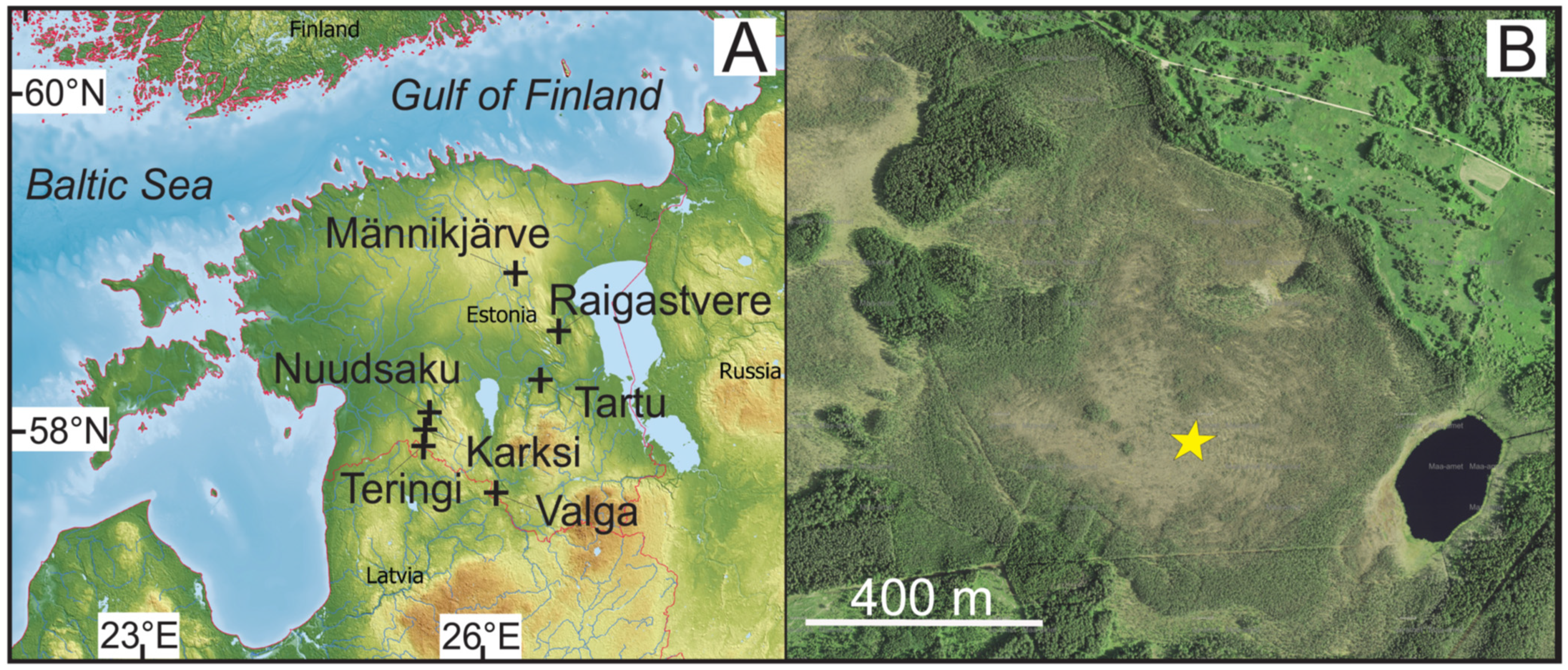
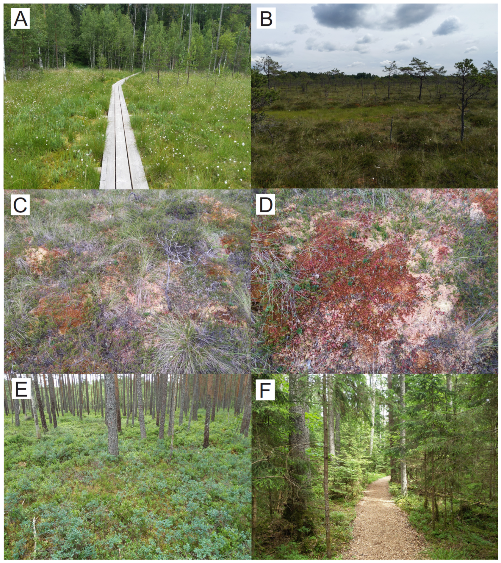
2. Study Site
3. Materials and Methods
3.1. Modern Hydrology
3.2. Modern Water Sampling
3.3. Core Sample Collection
3.4. Chronology
3.5. Species Identification
3.6. Carbon and Nitrogen Concentrations and Stable Isotopes
4. Results
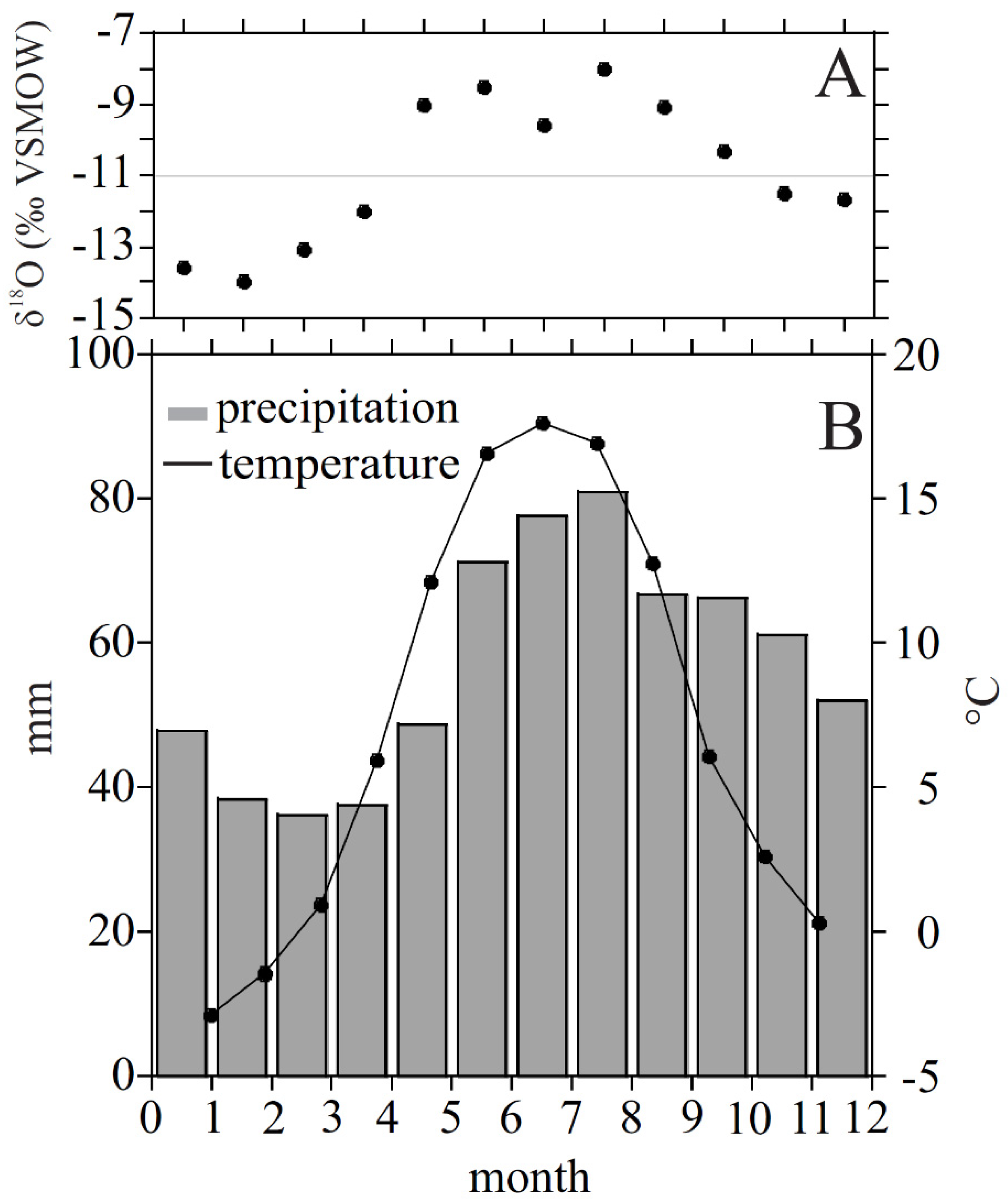
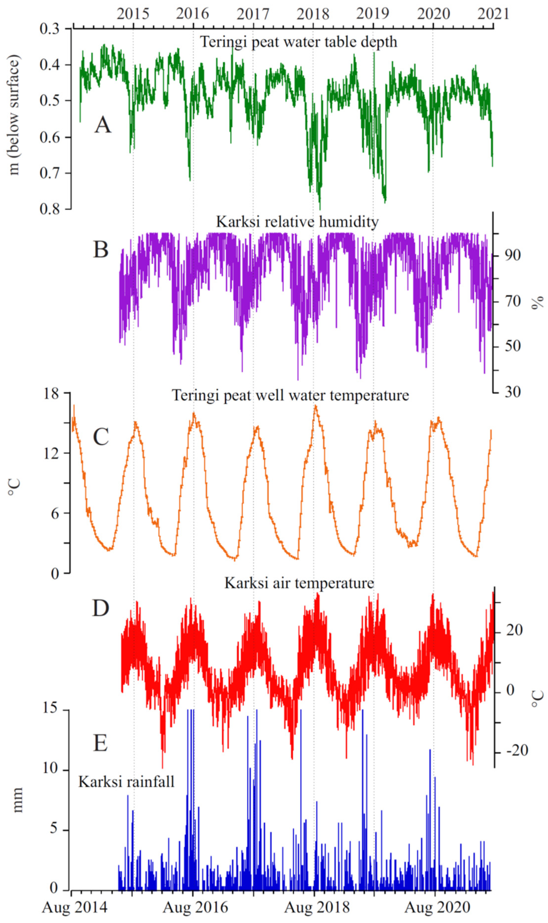
4.1. Weather Station Data
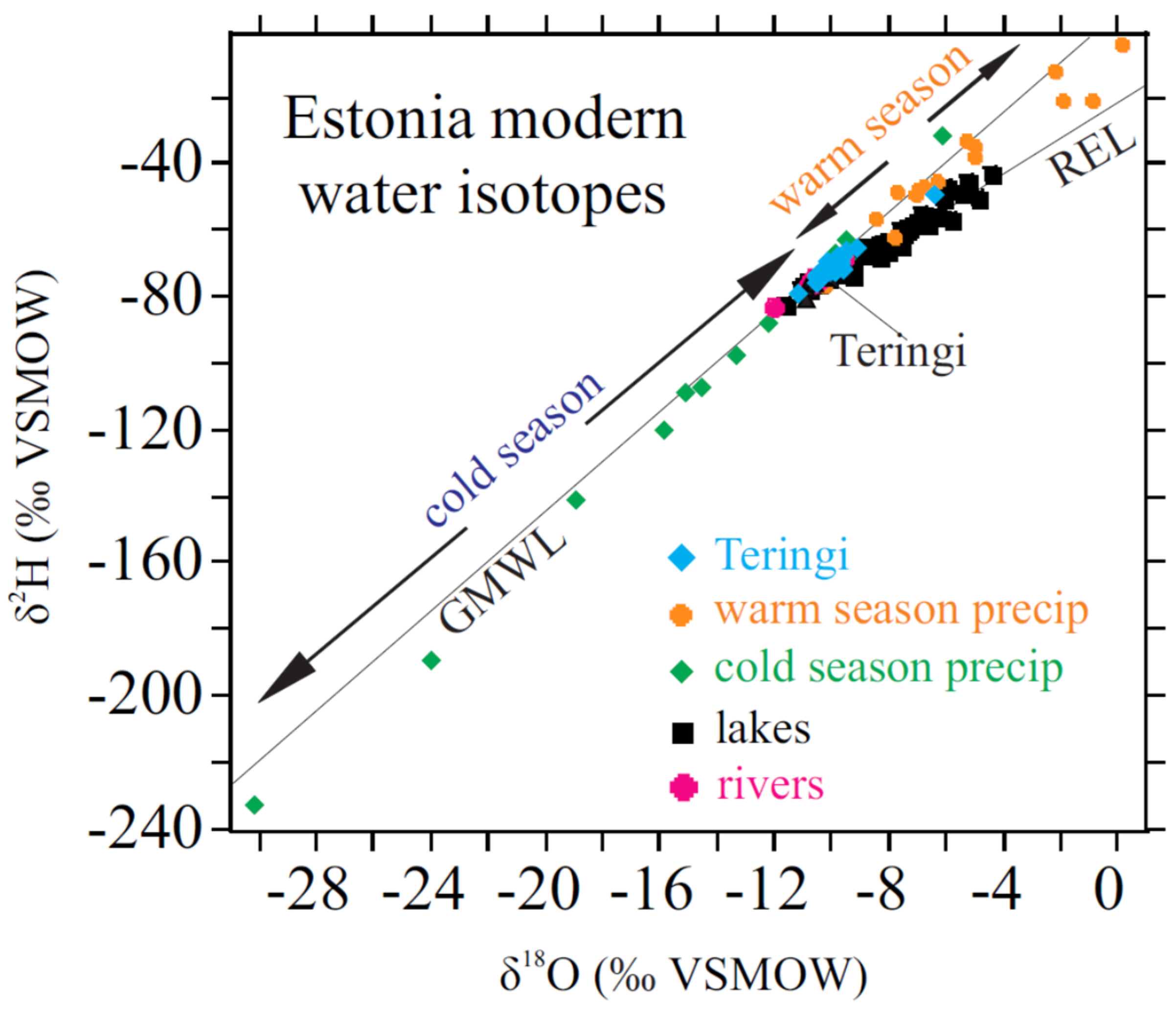
4.2. Surface Water and Precipitation Stable Isotopes
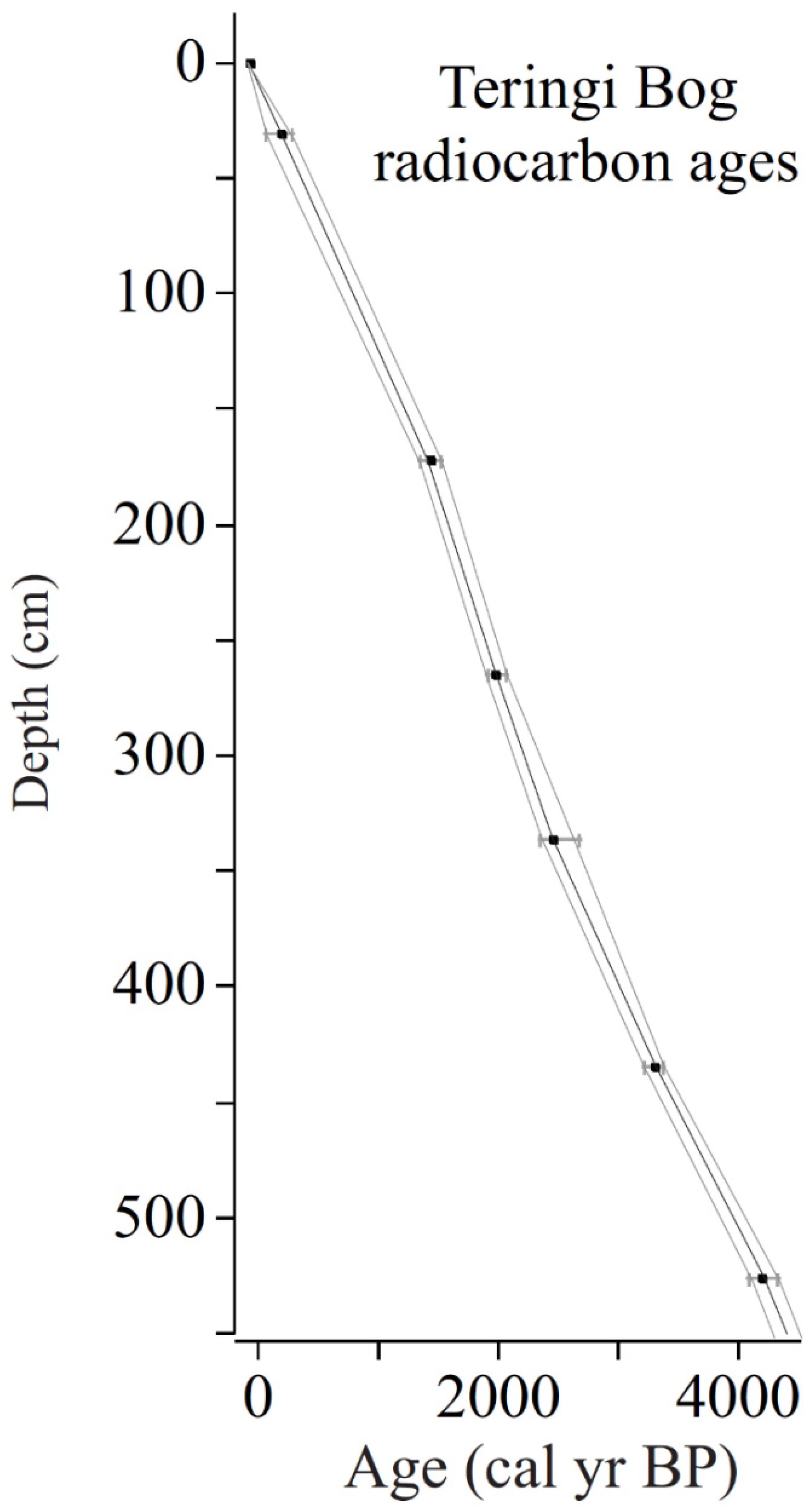
4.3. Chronology
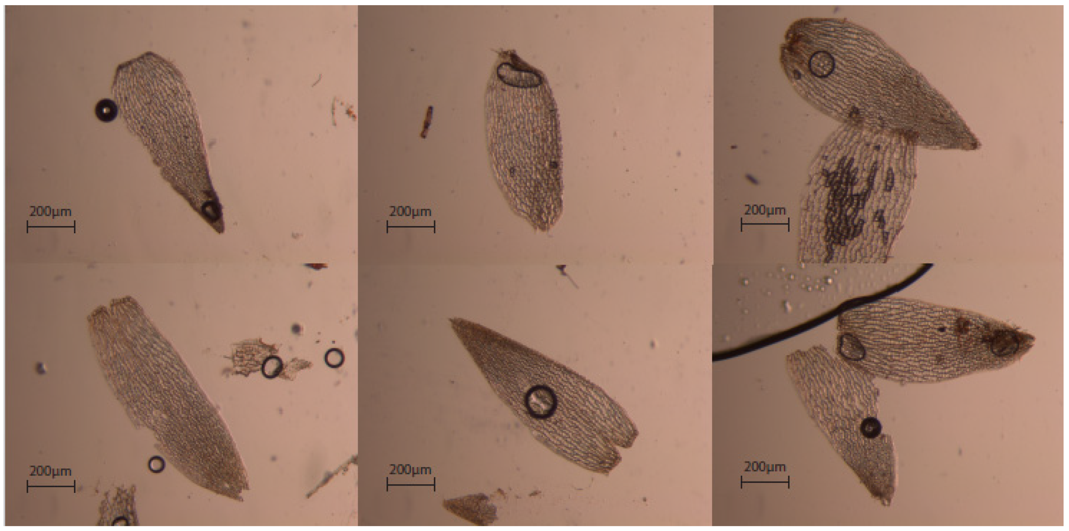
4.4. Species Identification
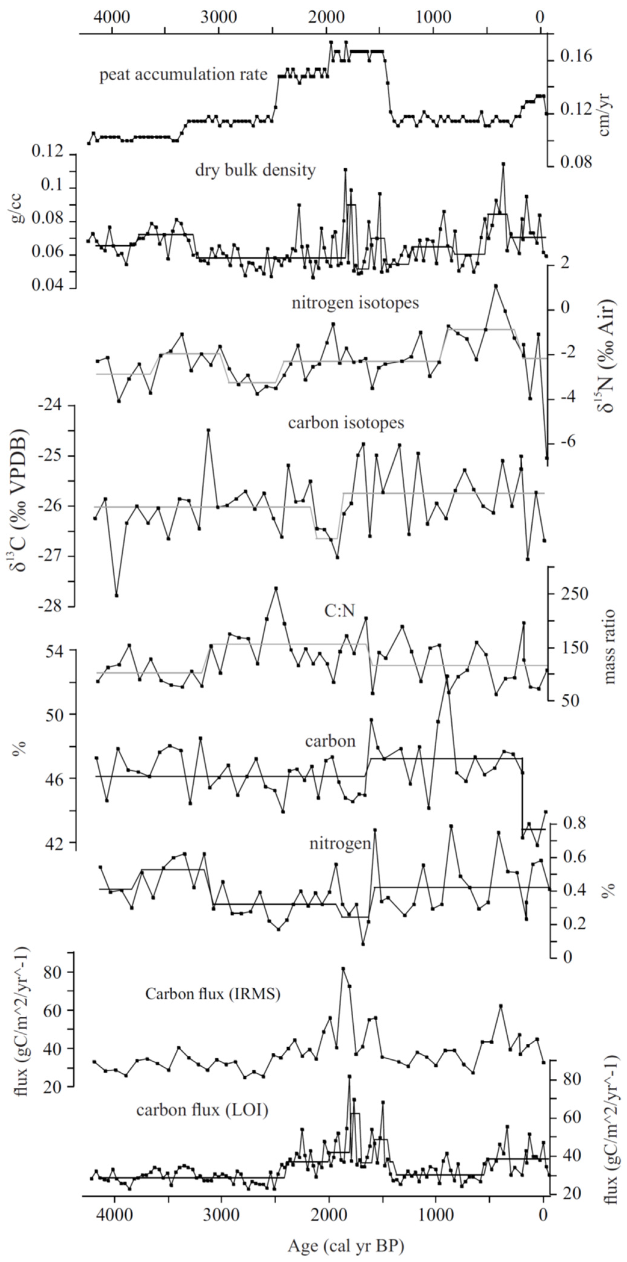
4.5. Peat Stable Isotope Records
4.6. Carbon, Nitrogen and Carbon Accumulation Rates
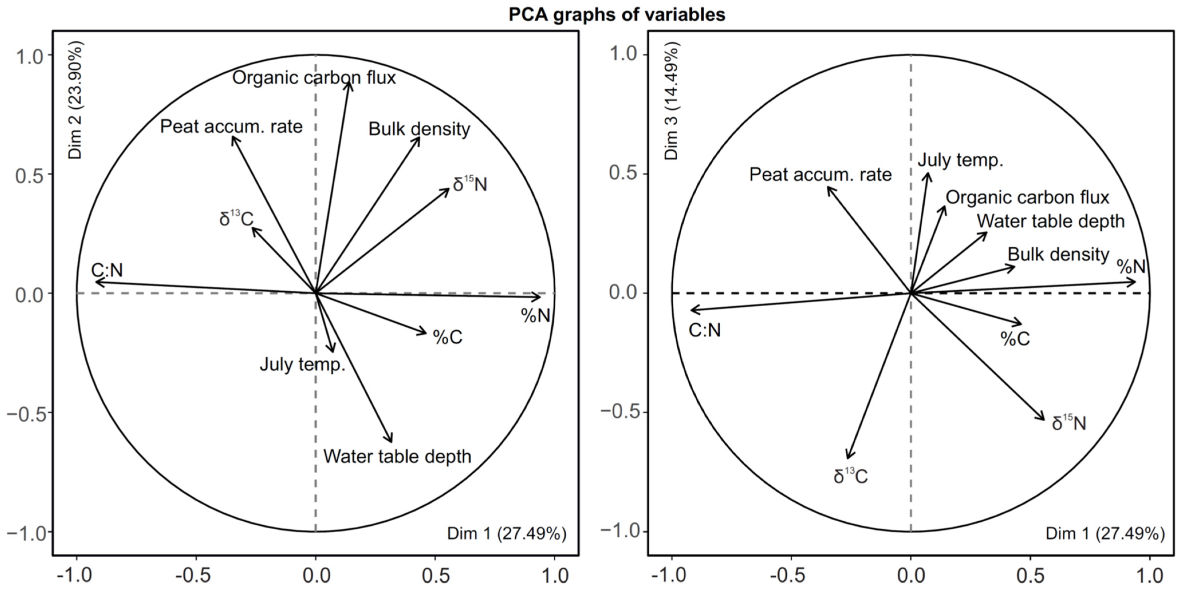
4.7. Principal Component Analysis
5. Discussion
5.1. Surface Water Source and Seasonality
5.2. Changes in Sphagnum
5.3. Carbon and Nitrogen Isotopes
5.4. Carbon Accumulation Rates and Hydrologic Conditions
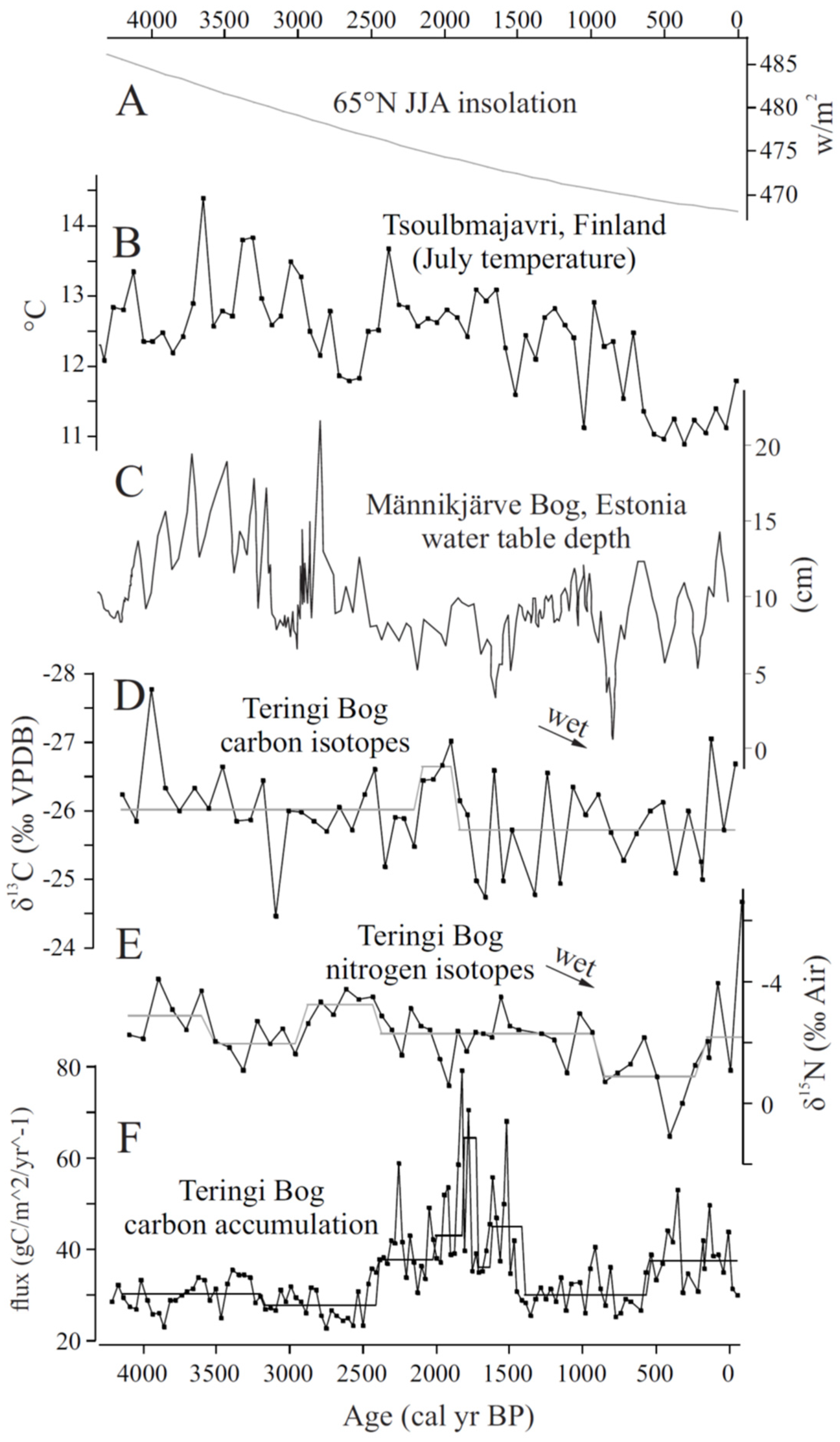
5.5. Climate Dynamics during the Late Holocene (4200 Cal Yr BP to Present)
5.6. Future Implications
6. Conclusions
Author Contributions
Funding
Data Availability Statement
Acknowledgments
Conflicts of Interest
References
- Gorham, E. Northern Peatlands: Role in the Carbon Cycle and Probable Responses to Climatic Warming. Ecol. Appl. 1991, 1, 182–195. [Google Scholar] [CrossRef]
- Turunen, J.; Tomppo, E.; Tolonen, K.; Reinikainen, A. Estimating carbon accumulation rates of undrained mires in Finland–application to boreal and subarctic regions. Holocene 2002, 12, 69–80. [Google Scholar] [CrossRef]
- Yu, Z.; Loisel, J.; Brosseau, D.P.; Beilman, D.W.; Hunt, S.J. Global peatland dynamics since the Last Glacial Maximum. Geophys. Res. Lett. 2010, 37, L13402. [Google Scholar] [CrossRef]
- Jobbágy, E.G.; Jackson, R.B. The vertical distribution of soil organic carbon and its relation to climate and vegetation. Ecol. Appl. 2000, 10, 423–436. [Google Scholar] [CrossRef]
- Battle, M.; Bender, M.; Tans, P.P.; White, J.; Ellis, J.; Conway, T.; Francey, R. Global carbon sinks and their variability inferred from atmospheric O2 and δ13C. Science 2000, 287, 2467–2470. [Google Scholar] [CrossRef] [PubMed] [Green Version]
- Grosse, G.; Harden, J.; Turetsky, M.; McGuire, A.D.; Camill, P.; Tarnocai, C.; Frolking, S.; Schuur, E.A.; Jorgenson, T.; Marchenko, S. Vulnerability of high-latitude soil organic carbon in North America to disturbance. J. Geophys. Res. Biogeosci. 2011, 116, G00K06. [Google Scholar] [CrossRef] [Green Version]
- Turetsky, M.R.; Kane, E.S.; Harden, J.W.; Ottmar, R.D.; Manies, K.L.; Hoy, E.; Kasischke, E.S. Recent acceleration of biomass burning and carbon losses in Alaskan forests and peatlands. Nat. Geosci. 2011, 4, 27–31. [Google Scholar] [CrossRef]
- Davidson, E.A.; Janssens, I.A. Temperature sensitivity of soil carbon decomposition and feedbacks to climate change. Nature 2006, 440, 165–173. [Google Scholar] [CrossRef] [PubMed]
- McGuire, A.; Hayes, D.J.; Kicklighter, D.W.; Manizza, M.; Zhuang, Q.; Chen, M.; Follows, M.J.; Gurney, K.; Mcclelland, J.W.; Melillo, J. An analysis of the carbon balance of the Arctic Basin from 1997 to 2006. Tellus B Chem. Phys. Meteorol. 2010, 62, 455–474. [Google Scholar] [CrossRef] [Green Version]
- Jones, M.C.; Yu, Z. Rapid deglacial and early Holocene expansion of peatlands in Alaska. Proc. Natl. Acad. Sci. USA 2010, 107, 7347–7352. [Google Scholar] [CrossRef] [Green Version]
- Frolking, S.; Roulet, N.T.; Tuittila, E.; Bubier, J.L.; Quillet, A.; Talbot, J.; Richard, P. A new model of Holocene peatland net primary production, decomposition, water balance, and peat accumulation. Earth Syst. Dyn. 2010, 1, 1–21. [Google Scholar] [CrossRef] [Green Version]
- Rydin, H.; Jeglum, J.K. The Biology of Peatlands, 2nd ed.; Oxford University Press: Oxford, UK, 2013. [Google Scholar]
- Clymo, R.; Bryant, C. Diffusion and mass flow of dissolved carbon dioxide, methane, and dissolved organic carbon in a 7-m deep raised peat bog. Geochim. Cosmochim. Acta 2008, 72, 2048–2066. [Google Scholar] [CrossRef]
- Tfaily, M.M.; Wilson, R.M.; Cooper, W.T.; Kostka, J.E.; Hanson, P.; Chanton, J.P. Vertical Stratification of Peat Pore Water Dissolved Organic Matter Composition in a Peat Bog in Northern Minnesota. J. Geophys. Res. Biogeosci. 2018, 123, 479–494. [Google Scholar] [CrossRef]
- Loisel, J.; Garneau, M.; Hélie, J.-F. Sphagnum δ13C values as indicators of palaeohydrological changes in a peat bog. Holocene 2010, 20, 285–291. [Google Scholar] [CrossRef]
- Stansell, N.D.; Klein, E.S.; Finkenbinder, M.S.; Fortney, C.S.; Dodd, J.P.; Terasmaa, J.; Nelson, D.B. A stable isotope record of Holocene precipitation dynamics in the Baltic region from Lake Nuudsaku, Estonia. Quat. Sci. Rev. 2017, 175, 73–84. [Google Scholar] [CrossRef]
- Asada, T.; Warner, B.G.; Aravena, R. Nitrogen isotope signature variability in plant species from open peatland. Aquat. Bot. 2005, 82, 297–307. [Google Scholar] [CrossRef]
- Laine, J.; Vasander, H. Ecology and vegetation gradients of peatlands. Peatl. Finl. 1996, 10, 20. [Google Scholar]
- Hugelius, G.; Loisel, J.; Chadburn, S.; Jackson, R.B.; Jones, M.; MacDonald, G.; Marushchak, M.; Olefeldt, D.; Packalen, M.; Siewert, M.B.; et al. Large stocks of peatland carbon and nitrogen are vulnerable to permafrost thaw. Proc. Natl. Acad. Sci. USA 2020, 117, 20438–20446. [Google Scholar] [CrossRef] [PubMed]
- Ives, S.L.; Sullivan, P.F.; Dial, R.; Berg, E.E.; Welker, J.M. CO2 exchange along a hydrologic gradient in the Kenai Lowlands, AK: Feedback implications of wetland drying and vegetation succession. Ecohydrology 2013, 6, 38–50. [Google Scholar] [CrossRef]
- Punning, J.M.; Toots, M.; Vaikmäe, R. Oxygen-18 in Estonian Natural Waters. Isot. Isot. Environ. Health Stud. 1987, 23, 232–234. [Google Scholar] [CrossRef]
- Klein, E.S.; Booth, R.K.; Yu, Z.; Mark, B.G.; Stansell, N.D. Hydrology-mediated differential response of carbon accumulation to late Holocene climate change at two peatlands in Southcentral Alaska. Quat. Sci. Rev. 2013, 64, 61–75. [Google Scholar] [CrossRef]
- Berger, A.; Loutre, M.F. Insolation values for the climate of the last 10 million years. Quat. Sci. Rev. 1991, 10, 297–317. [Google Scholar] [CrossRef]
- Paal, J. Rare and threatened plant communities of Estonia. Biodivers. Conserv. 1998, 7, 1027–1049. [Google Scholar] [CrossRef]
- Kalm, V. Pleistocene chronostratigraphy in Estonia, southeastern sector of the Scandinavian glaciation. Quat. Sci. Rev. 2006, 25, 960–975. [Google Scholar] [CrossRef]
- Masing, V.; Paal, J.; Kuresoo, A. Biodiversity of Estonian wetlands. Biodivers. Wetl. Assess. Funct. Conserv. 2000, 1, 259–279. [Google Scholar]
- Paal, J. Estonian mires. Mires—Sib. Tierra Del Fuego. Stapfia85 Zugleich Kat. Der OO. Landesmuseen Neue Ser. 2005, 35, 117–146. [Google Scholar]
- Jaagus, J. The impact of climate change on the snow cover pattern in Estonia. Clim. Change 1997, 36, 65–77. [Google Scholar] [CrossRef]
- Jaagus, J. Climatic changes in Estonia during the second half of the 20th century in relationship with changes in large-scale atmospheric circulation. Theor. Appl. Climatol. 2006, 83, 77–88. [Google Scholar] [CrossRef]
- Bladé, I.; Liebmann, B.; Fortuny, D.; Oldenborgh, G. Observed and simulated impacts of the summer NAO in Europe: Implications for projected drying in the Mediterranean region. Clim. Dyn. 2012, 39, 709–727. [Google Scholar] [CrossRef]
- Mätlik, O.; Post, P. Synoptic Weather Types That Have Caused Heavy Precipitation in Estonia in the Period 1961-2005. Est. J. Eng. 2008, 14, 195–208. [Google Scholar] [CrossRef] [Green Version]
- Wassenaar, L.I.; Coplen, T.B.; Aggarwal, P.K. Approaches for Achieving Long-Term Accuracy and Precision of δ18O and δ2H for Waters Analyzed using Laser Absorption Spectrometers. Environ. Sci. Technol. 2014, 48, 1123–1131. [Google Scholar] [CrossRef] [PubMed]
- Coplen, T.B. Guidelines and recommended terms for expression of stable-isotope-ratio and gas-ratio measurement results. Rapid Commun. Mass Spectrom. 2011, 25, 2538–2560. [Google Scholar] [CrossRef]
- Reimer, P.J.; Austin, W.E.; Bard, E.; Bayliss, A.; Blackwell, P.G.; Ramsey, C.B.; Butzin, M.; Cheng, H.; Edwards, R.L.; Friedrich, M. The IntCal20 Northern Hemisphere radiocarbon age calibration curve (0–55 cal kBP). Radiocarbon 2020, 62, 725–757. [Google Scholar] [CrossRef]
- Blaauw, M.; Christen, J.A. Flexible paleoclimate age-depth models using an autoregressive gamma process. Bayesian Anal. 2011, 6, 457–474. [Google Scholar] [CrossRef]
- Laine, J.; Harju, P.; Timonen, T.; Laine, A.; Tuittila, E.-S.; Minkkinen, K.; Vasander, H. The Intricate Beauty of Sphagnum Mosses—A Finnish Guide to Identification; University of Helsinki, Department of Forest Ecology: Helsinki, Finland, 2009. [Google Scholar]
- Loader, N.; McCarroll, D.; van der Knaap, W.O.; Robertson, I.; Gagen, M. Characterizing carbon isotopic variability in Sphagnum. Holocene 2007, 17, 403–410. [Google Scholar] [CrossRef]
- Dean, W.E. Determination of carbonate and organic matter in calcareous sediments and sedimentary rocks by loss on ignition: Comparison with other methods. J. Sediment. Petrol. 1974, 44, 242–248. [Google Scholar]
- Heiri, O.; Lotter, A.F.; Lemcke, G. Loss on ignition as a method for estimating organic and carbonate content in sediments: Reproducibility and comparability of results. J. Paleolimnol. 2001, 25, 101–110. [Google Scholar] [CrossRef]
- Boyle, J. A comparison of two methods for estimating the organic matter content of sediments. J. Paleolimnol. 2004, 31, 125–127. [Google Scholar]
- Loisel, J.; Yu, Z.; Beilman, D.W.; Camill, P.; Alm, J.; Amesbury, M.J.; Anderson, D.; Andersson, S.; Bochicchio, C.; Barber, K.; et al. A database and synthesis of northern peatland soil properties and Holocene carbon and nitrogen accumulation. Holocene 2014, 24, 1028–1042. [Google Scholar] [CrossRef]
- Rodionov, S.N. A sequential algorithm for testing climate regime shifts. Geophys. Res. Lett. 2004, 31, L09204. [Google Scholar] [CrossRef] [Green Version]
- Lê, S.; Josse, J.; Husson, F. FactoMineR: An R package for multivariate analysis. J. Stat. Softw. 2008, 25, 1–18. [Google Scholar] [CrossRef] [Green Version]
- Seppä, H.; Birks, H.J.B. July mean temperature and annual precipitation trends during the Holocene in the Fennoscandian tree-line area: Pollen-based climate reconstructions. Holocene 2001, 11, 527–539. [Google Scholar] [CrossRef] [Green Version]
- Sillasoo, U.; Mauquoy, D.; Blundell, A.; Charman, D.A.N.; Blaauw, M.; Daniell, J.R.G.; Toms, P.; Newberry, J.; Chambers, F.M.; Karofeld, E. Peat multi-proxy data from Männikjärve bog as indicators of late Holocene climate changes in Estonia. Boreas 2007, 36, 20–37. [Google Scholar] [CrossRef]
- Hill, K. Late Holocene Climate Controls on Carbon Dynamics at Teringi Bog, Estonia; Northern Illinois University: DeKalb, IL, USA, 2016. [Google Scholar]
- Ménot, G.; Burns, S.J. Carbon isotopes in ombrogenic peat bog plants as climatic indicators: Calibration from an altitudinal transect in Switzerland. Org. Geochem. 2001, 32, 233–245. [Google Scholar] [CrossRef]
- Dansgaard, W. Stable isotopes in precipitation. Tellus 1964, 16, 436–468. [Google Scholar] [CrossRef]
- Rozanski, K.; Araquás-Araquás, L.; Gonfiantini, R. Relation Between Long-Term Trends of Oxygen-18 Isotope Composition of Precipitation and Climate. Science 1992, 258, 981–985. [Google Scholar] [CrossRef]
- Baldini, L.M.; McDermott, F.; Foley, A.M.; Baldini, J.U.L. Spatial variability in the European winter precipitation δ18O-NAO relationship: Implications for reconstructing NAO-mode climate variability in the Holocene. Geophys. Res. Lett. 2008, 35, L04709. [Google Scholar] [CrossRef]
- St Amour, N.A.; Hammarlund, D.; Edwards, T.W.; Wolfe, B.B. New insights into Holocene atmospheric circulation dynamics in central Scandinavia inferred from oxygen-isotope records of lake-sediment cellulose. Boreas 2010, 39, 770–782. [Google Scholar] [CrossRef]
- Hammarlund, D.; Björck, S.; Buchardt, B.; Israelson, C.; Thomsen, C.T. Rapid hydrological changes during the Holocene revealed by stable isotope records of lacustrine carbonates from Lake Igelsjön, southern Sweden. Quat. Sci. Rev. 2003, 22, 353–370. [Google Scholar] [CrossRef]
- Heikkilä, M.; Edwards, T.W.D.; Seppä, H.; Sonninen, E. Sediment isotope tracers from Lake Saarikko, Finland, and implications for Holocene hydroclimatology. Quat. Sci. Rev. 2010, 29, 2146–2160. [Google Scholar] [CrossRef]
- Luken, J.O. Zonation of Sphagnum Mosses: Interactions among Shoot Growth, Growth Form, and Water Balance. Bryologist 1985, 88, 374–379. [Google Scholar] [CrossRef]
- Robroek, B.J.M.; Limpens, J.; Breeuwer, A.; Schouten, M.G.C. Effects of water level and temperature on performance of four Sphagnum mosses. Plant Ecol. 2007, 190, 97–107. [Google Scholar] [CrossRef]
- Hájek, T.; Beckett, R.P. Effect of water content components on desiccation and recovery in Sphagnum mosses. Ann. Bot. 2008, 101, 165–173. [Google Scholar] [CrossRef] [PubMed] [Green Version]
- Payette, S. Late-Holocene development of subarctic ombrotrophic peatlands: Allogenic and autogenic succession. Ecology 1988, 69, 516–531. [Google Scholar] [CrossRef]
- Rastogi, A.; Antala, M.; Gąbka, M.; Rosadziński, S.; Stróżecki, M.; Brestic, M.; Juszczak, R. Impact of warming and reduced precipitation on morphology and chlorophyll concentration in peat mosses (Sphagnum angustifolium and S. fallax). Sci. Rep. 2020, 10, 8592. [Google Scholar] [CrossRef]
- Moschen, R.; Kühl, N.; Rehberger, I.; Lücke, A. Stable carbon and oxygen isotopes in sub-fossil Sphagnum: Assessment of their applicability for palaeoclimatology. Chem. Geol. 2009, 259, 262–272. [Google Scholar] [CrossRef]
- Ménot-Combes, G.; Burns, S.J.; Leuenberger, M. Variations of 18O/16O in plants from temperate peat bogs (Switzerland): Implications for paleoclimatic studies. Earth Planet. Sci. Lett. 2002, 202, 419–434. [Google Scholar] [CrossRef]
- Melillo, J.M.; Aber, J.D.; Linkins, A.E.; Ricca, A.; Fry, B.; Nadelhoffer, K.J. Carbon and nitrogen dynamics along the decay continuum: Plant litter to soil organic matter. Plant. Soil 1989, 115, 189–198. [Google Scholar] [CrossRef]
- Malmer, N.; Svensson, G.; Wallén, B. Mass balance and nitrogen accumulation in hummocks on a South Swedish bog during the late Holocene. Ecography 1997, 20, 535–549. [Google Scholar] [CrossRef]
- Kuhry, P.; Vitt, D.H. Fossil Carbon/Nitrogen Ratios as a Measure of Peat Decomposition. Ecology 1996, 77, 271–275. [Google Scholar] [CrossRef]
- Ohlson, M.; Dahlberg, B. Rate of peat increment in hummock and lawn communities on Swedish mires during the last 150 years. Oikos 1991, 61, 369–378. [Google Scholar] [CrossRef]
- Berger, A.L. Long-term variations of caloric insolation resulting from the Earth’s orbital elements. Quat. Res. 1978, 9, 139–167. [Google Scholar] [CrossRef]
- Seppä, H.; Poska, A. Holocene annual mean temperature changes in Estonia and their relationship to solar insolation and atmospheric circulation patterns. Quat. Res. 2004, 61, 22–31. [Google Scholar] [CrossRef]
- Walker, M.J.C.; Berkelhammer, M.; Björck, S.; Cwynar, L.C.; Fisher, D.A.; Long, A.J.; Lowe, J.J.; Newnham, R.M.; Rasmussen, S.O.; Weiss, H. Formal subdivision of the Holocene Series/Epoch: A Discussion Paper by a Working Group of INTIMATE (Integration of ice-core, marine and terrestrial records) and the Subcommission on Quaternary Stratigraphy (International Commission on Stratigraphy). J. Quat. Sci. 2012, 27, 649–659. [Google Scholar] [CrossRef]
- Morley, A.; Rosenthal, Y.; deMenocal, P. Ocean-atmosphere climate shift during the mid-to-late Holocene transition. Earth Planet. Sci. Lett. 2014, 388, 18–26. [Google Scholar] [CrossRef] [Green Version]
- Cowling, S.A.; Sykes, M.T.; Bradshaw, R.H.W. Palaeovegetation-model comparisons, climate change and tree succession in Scandinavia over the past 1500 years. J. Ecol. 2001, 89, 227–236. [Google Scholar] [CrossRef] [Green Version]
- Poska, A.; Saarse, L.; Koppel, K.; Nielsen, A.B.; Avel, E.; Vassiljev, J.; Väli, V. The Verijärv area, South Estonia over the last millennium: A high resolution quantitative land-cover reconstruction based on pollen and historical data. Rev. Palaeobot. Palynol. 2014, 207, 5–17. [Google Scholar] [CrossRef]
- Helama, S.; Meriläinen, J.; Tuomenvirta, H. Multicentennial megadrought in northern Europe coincided with a global El Niño–Southern Oscillation drought pattern during the Medieval Climate Anomaly. Geology 2009, 37, 175–178. [Google Scholar] [CrossRef] [Green Version]
- Luoto, T.P.; Helama, S. Palaeoclimatological and palaeolimnological records from fossil midges and tree-rings: The role of the North Atlantic Oscillation in eastern Finland through the Medieval Climate Anomaly and Little Ice Age. Quat. Sci. Rev. 2010, 29, 2411–2423. [Google Scholar] [CrossRef]
- Tiljander, M.I.A.; Saarnisto, M.; Ojala, A.E.K.; Saarinen, T. A 3000-year palaeoenvironmental record from annually laminated sediment of Lake Korttajarvi, central Finland. Boreas 2003, 32, 566–577. [Google Scholar] [CrossRef]
- Tarand, A.; Nordli, P.Ø. The Tallinn Temperature Series Reconstructed Back Half a Millennium by Use of Proxy Data. In The Iceberg in the Mist: Northern Research in Pursuit of a “Little Ice Age”; Ogilvie, A.E.J., Jónsson, T., Eds.; Springer: Dordrecht, The Netherlands, 2001; pp. 189–199. [Google Scholar]
- Stouffer, R.J.; Manabe, S. Response of a Coupled Ocean–Atmosphere Model to Increasing Atmospheric Carbon Dioxide: Sensitivity to the Rate of Increase. J. Clim. 1999, 12, 2224–2237. [Google Scholar] [CrossRef] [Green Version]
- BACC. Assessment of Climate Change for the Baltic Sea Basin; Germany, 2008; Available online: https://link.springer.com/book/10.1007/978-3-540-72786-6 (accessed on 1 August 2021).
- EEA. European Environment Agency: National Adaptation Policy Processes in European Countries 2014. 2014; Available online: https://www.eea.europa.eu/publications/national-adaptation-policy-processes (accessed on 1 August 2021).
- IPCC. Climate Change 2014: Impacts, Adaptation, and Vulnerability. Part. B: Regional Aspects. Contribution of Working Group II to the Fifth Assessment Report of the Intergovernmental Panel on Climate Change; Barros, V.R.C.B., Field, D.J., Dokken, M.D., Mastrandrea, K.J., Mach., T.E., Bilir, M., Chatterjee, K.L., Ebi, Y.O., Estrada, R.C., Genova, B., et al., Eds.; Cambridge University Press: Cambridge, UK; New York, NY, USA, 2014. [Google Scholar]
- Kont, A.; Jaagus, J.; Aunap, R. Climate change scenarios and the effect of sea-level rise for Estonia. Glob. Planet. Change 2003, 36, 1–15. [Google Scholar] [CrossRef]
- Kauker, F.; Meier, H.E.M. Modeling decadal variability of the Baltic Sea: 1. Reconstructing atmospheric surface data for the period 1902–1998. J. Geophys. Res. Ocean. 2003, 108, 3267. [Google Scholar] [CrossRef] [Green Version]
- Meier, H.E.M.; Kauker, F. Modeling decadal variability of the Baltic Sea: 2. Role of freshwater inflow and large-scale atmospheric circulation for salinity. J. Geophys. Res. Ocean. 2003, 108, 3368. [Google Scholar] [CrossRef] [Green Version]
- Meier, H.E.M. Baltic Sea climate in the late twenty-first century: A dynamical downscaling approach using two global models and two emission scenarios. Clim. Dyn. 2006, 27, 39–68. [Google Scholar] [CrossRef]
- Harrison, S.P.; Bartlein, P.J.; Izumi, K.; Li, G.; Annan, J.; Hargreaves, J.; Braconnot, P.; Kageyama, M. Evaluation of CMIP5 palaeo-simulations to improve climate projections. Nat. Clim. Change 2015, 5, 735–743. [Google Scholar] [CrossRef]
- Rutgersson, A.; Jaagus, J.; Schenk, F.; Stendel, M. Observed changes and variability of atmospheric parameters in the Baltic Sea region during the last 200 years. Clim. Res. 2014, 61, 177–190. [Google Scholar] [CrossRef] [Green Version]
- Graham, L.P. Climate Change Effects on River Flow to the Baltic Sea. AMBIO A J. Hum. Environ. 2004, 33, 235–241. [Google Scholar] [CrossRef]
- Collins, M.; Knutti, R.; Arblaster, J.; Dufresne, J.-L.; Fichefet, T.; Friedlingstein, P.; Gao, X.; Gutowski, W.J.; Johns, T.; Krinner, G. Long-term climate change: Projections, commitments and irreversibility. In Climate Change 2013-The Physical Science Basis: Contribution of Working Group I to the Fifth Assessment Report of the Intergovernmental Panel on Climate Change; Cambridge University Press: Cambridge, UK, 2013; pp. 1029–1136. [Google Scholar]


| 14C Age | Analytical Uncertainty ± 1σ | Median Calibrated Age (cal yr BP) | Minimum Calibrated Age (cal yr BP) 2σ | Maximum Calibrated Age (cal yr BP) 2σ | Weighted Mean Modeled Age (cal yr BP) | Minimum Modeled Age (cal yr BP) 2σ | Maximum Modeled Age (cal yr BP) 2σ |
|---|---|---|---|---|---|---|---|
| –65 | 1 | –65 | –68 | –62 | |||
| 140 | 15 | 109 | 58 | 118 | 172 | 63 | 271 |
| 1545 | 15 | 1405 | 1369 | 1419 | 1401 | 1351 | 1488 |
| 2025 | 15 | 1963 | 1925 | 2000 | 1968 | 1901 | 2043 |
| 2380 | 20 | 2392 | 2346 | 2465 | 2442 | 2352 | 2654 |
| 3075 | 15 | 3291 | 3232 | 3358 | 3297 | 3218 | 3363 |
| 3810 | 20 | 4195 | 4145 | 4252 | 4200 | 4097 | 4347 |
| Section Acutifolia | Section Cuspidata | Section Subsecunda | Section Sphagnum | |||||||||
|---|---|---|---|---|---|---|---|---|---|---|---|---|
| Depth (cm) | Age (cal yr BP) | S. fuscum | S. capilli-folium | S. rubellum | S. russowi | S. pulchrum | S. fallax | S. angusti-folium | S.balticum | S. lind-bergii | spp. | S. medium |
| 32 | 182 | 2 | 2 | |||||||||
| 42 | 266 | 2 | 1 | |||||||||
| 52 | 352 | 1 | 2 | 2 | ||||||||
| 62 | 439 | 1 | 2 | |||||||||
| 72 | 525 | 1 | ||||||||||
| 82 | 613 | 2 | 2 | 2 | ||||||||
| 92 | 699 | 2 | 2 | 2 | 2 | |||||||
| 102 | 786 | 2 | 1 | |||||||||
| 112 | 870 | 1 | ||||||||||
| 122 | 957 | 2 | 1 | |||||||||
| 132 | 1042 | 1 | ||||||||||
| 142 | 1130 | 1 | 2 | 2 | ||||||||
| 152 | 1220 | 1 | 2 | |||||||||
| 162 | 1311 | 2 | 2 | 1 | ||||||||
| 172 | 1397 | 1 | 2 | |||||||||
| 182 | 1460 | 1 | 2 | 2 | 2 | |||||||
| 192 | 1521 | 1 | 2 | |||||||||
| 202 | 1581 | 1 | ||||||||||
| 212 | 1642 | 2 | 2 | 1 | ||||||||
| 222 | 1701 | 1 | 1 | 2 | ||||||||
| 232 | 1762 | 1 | 1 | 2 | ||||||||
| 242 | 1823 | 2 | 1 | |||||||||
| 252 | 1885 | 2 | 1 | |||||||||
| 262 | 1946 | 1 | 2 | 2 | ||||||||
| 272 | 2011 | 1 | 2 | |||||||||
| 282 | 2078 | 1 | 2 | |||||||||
| 292 | 2144 | 1 | 2 | |||||||||
| 302 | 2210 | 1 | 2 | |||||||||
| 312 | 2276 | 1 | 2 | 1 | ||||||||
| 322 | 2343 | 1 | ||||||||||
| 332 | 2411 | 1 | 2 | 2 | ||||||||
| 342 | 2487 | 1 | 2 | 2 | ||||||||
| 352 | 2575 | 1 | 2 | 2 | ||||||||
| 362 | 2663 | 1 | 2 | |||||||||
| 372 | 2750 | 2 | 1 | |||||||||
| 382 | 2837 | 2 | 1 | |||||||||
| 392 | 2923 | 2 | 1 | 2 | ||||||||
| 402 | 3011 | 1 | 2 | |||||||||
| 412 | 3099 | 1 | 2 | |||||||||
| 422 | 3187 | 1 | 2 | |||||||||
| 432 | 3275 | 1 | 2 | |||||||||
| 442 | 3370 | 1 | ||||||||||
| 452 | 3469 | 1 | 2 | |||||||||
| 462 | 3567 | 1 | ||||||||||
| 472 | 3665 | 1 | 1 | |||||||||
| 482 | 3764 | 1 | ||||||||||
| 492 | 3862 | 1 | 1 | |||||||||
| 502 | 3959 | 1 | 2 | 1 | ||||||||
| 512 | 4055 | 1 | ||||||||||
| 522 | 4154 | 1 | ||||||||||
| Variable | Dim. 1 | Dim. 2 | Dim. 3 |
|---|---|---|---|
| %N | 0.938 | −0.016 | 0.048 |
| C:N | −0.918 | 0.047 | −0.072 |
| õ15N | 0.557 | 0.439 | −0.531 |
| Organic C flux | 0.141 | 0.884 | 0.365 |
| Peat accum. Rate | −0.347 | 0.657 | 0.446 |
| Bulk density | 0.433 | 0.654 | 0.111 |
| Water table depth | 0.316 | −0.624 | 0.255 |
| õ13C | −0.264 | 0.274 | −0.692 |
| July temp | 0.072 | −0.246 | 0.504 |
| %C | 0.461 | −0.168 | −0.13 |
Publisher’s Note: MDPI stays neutral with regard to jurisdictional claims in published maps and institutional affiliations. |
© 2022 by the authors. Licensee MDPI, Basel, Switzerland. This article is an open access article distributed under the terms and conditions of the Creative Commons Attribution (CC BY) license (https://creativecommons.org/licenses/by/4.0/).
Share and Cite
Stansell, N.D.; Klein, E.S.; Hill, K.; Terasmaa, J.; Dodd, J.; Boes, M.; Eensalu, M.; Fortney, C.; Fritts, A.; Garcia, R.; et al. A Late Holocene Stable Isotope and Carbon Accumulation Record from Teringi Bog in Southern Estonia. Quaternary 2022, 5, 8. https://doi.org/10.3390/quat5010008
Stansell ND, Klein ES, Hill K, Terasmaa J, Dodd J, Boes M, Eensalu M, Fortney C, Fritts A, Garcia R, et al. A Late Holocene Stable Isotope and Carbon Accumulation Record from Teringi Bog in Southern Estonia. Quaternary. 2022; 5(1):8. https://doi.org/10.3390/quat5010008
Chicago/Turabian StyleStansell, Nathan D., Eric S. Klein, Kristyn Hill, Jaanus Terasmaa, Justin Dodd, Maxwell Boes, Mariliis Eensalu, Carolyn Fortney, Annabella Fritts, Roxana Garcia, and et al. 2022. "A Late Holocene Stable Isotope and Carbon Accumulation Record from Teringi Bog in Southern Estonia" Quaternary 5, no. 1: 8. https://doi.org/10.3390/quat5010008