Classifying Breast Tumors in Digital Tomosynthesis by Combining Image Quality-Aware Features and Tumor Texture Descriptors

Abstract

Digital breast tomosynthesis (DBT) is a 3D breast cancer screening technique that can overcome the limitations of standard 2D digital mammography. However, DBT images often suffer from artifacts stemming from acquisition conditions, a limited angular range, and low radiation doses. These artifacts have the potential to degrade the performance of automated breast tumor classification tools. Notably, most existing automated breast tumor classification methods do not consider the effect of DBT image quality when designing the classification models. In contrast, this paper introduces a novel deep learning-based framework for classifying breast tumors in DBT images. This framework combines global image quality-aware features with tumor texture descriptors. The proposed approach employs a two-branch model: in the top branch, a deep convolutional neural network (CNN) model is trained to extract robust features from the region of interest that includes the tumor. In the bottom branch, a deep learning model named TomoQA is trained to extract global image quality-aware features from input DBT images. The quality-aware features and the tumor descriptors are then combined and fed into a fully-connected layer to classify breast tumors as benign or malignant. The unique advantage of this model is the combination of DBT image quality-aware features with tumor texture descriptors, which helps accurately classify breast tumors as benign or malignant. Experimental results on a publicly available DBT image dataset demonstrate that the proposed framework achieves superior breast tumor classification results, outperforming all existing deep learning-based methods.

1. Introduction

Worldwide, breast cancer has emerged as a leading cause of mortality, posing a threat to women every year [1]. Clinical studies have shown that the early detection and classification of breast cancers markedly enhance patient treatment and therapy outcomes [2,3]. Medical imaging techniques, including mammography, computed tomography (CT), magnetic resonance imaging (MRI), and breast ultrasound (BUS), typically play a crucial role in the assessment of breast cancer [4]. Mammography is the standard modality for detecting breast cancer in its early stages [5]. However, mammography exhibits a high false positive rate, wherein normal tissue is incorrectly identified as an abnormal. This is attributed to the overlap of normal fibroglandular tissues in 2D imaging and the occurrence of cancer-like abnormalities, leading to unnecessary additional biopsies [6].

Digital breast tomosynthesis (DBT) offers a solution to the limitations of mammography [7]. DBT can be regarded as a subset of the mammography procedure, differing in that the X-ray tube in breast tomosynthesis sweeps in an arc around the compressed breast, capturing multiple images (slices) from various angles [8]. DBT plays a crucial role in reducing the false positive rate by minimizing tissue overlap, which can conceal cancers or complicate the differentiation between normal overlapping breast tissue and tumors [9].

The analysis of a large volume of DBT is labor-intensive and time-consuming for radiologists. To overcome such challenges, numerous automated tools and computer-aided diagnosis (CAD) systems have been proposed to assist radiologists in detecting and diagnosing breast cancer in DBT images [10,11,12,13]. In recent years, several CAD systems based on deep convolutional neural networks (CNNs), like [14,15,16,17], have been introduced for the detection and classification of breast tumors in DBT images. Notably, the majority of previous studies have been conducted on in-house DBT datasets, thus limiting the reproducibility of the results. Therefore, it is imperative to utilize publicly available DBT datasets when developing a reliable CAD system.

Despite the superior quality of DBT images compared with mammography and breast ultrasound ones, various artifacts can significantly degrade the image quality of DBT images. These artifacts arise from factors such as acquisition conditions, a limited angular range, a low radiation dose, and reconstruction processes [18]. To elucidate these artifacts, Figure 1 showcases four instances of DBT images, each highlighting distinct artifacts impacting the quality of DBT. Notably, patient motion during the acquisition process can cause blurring and ghosting in the image, altering the appearance of tumors (indicated by the green arrow and box). Additionally, the influence of scatter radiation is evident, contributing to diminished image contrast and clarity, a consequence of low or high radiation doses (depicted by blue and red arrows and boxes). The final image underscores the impact of missing information in image reconstruction, leading to noisy DBT images that manifest as bright or dark pixels.

Most existing CAD systems are constrained to the classification of breast tissue as normal or abnormal, paying limited attention to distinguishing between benign and malignant breast tumors. Furthermore, most existing automated breast tumor classification methods do not consider the effect of DBT image quality when designing the classification models. In an effort to enhance breast tumor classification accuracy, this paper introduces a new deep learning-based framework for classifying breast tumors in DBT images. This framework integrates global image quality-aware features with tumor texture descriptors. The proposed framework employs a two-branch model: in the top branch, a CNN model is trained to extract robust features from the region of interest, which includes the tumor. Concurrently, in the bottom branch, a deep learning model called TomoQA is trained to extract global image quality-aware features from the input DBT images. Subsequently, the quality-aware features and tumor descriptors are combined and input into a fully-connected layer to classify breast tumors as either benign or malignant.

The following enumerates the main novelties of this study:

• Presenting a novel deep learning-based framework for breast tumor classification in DBT images. The unique merit of this model is the combination of DBT image quality-aware features with tumor texture descriptors, which helps accurately categorize the breast tumor as benign or malignant.
• Proposing the TomoQA deep learning model to extract quality-aware features from DBT images.
• Conducting an extensive experimental analysis on a publicly available DBT dataset and providing comparisons with existing methods to demonstrate the superiority of the proposed method. The implementation code for our proposed method from this study is publicly available on GitHub at https://github.com/loaysh2010/Classifying-Breast-Tumors-in-DBT-Images-based-on-Image-Quality-Aware-Features, accessed on 6 March 2024.

Section 2 discusses the related work of breast cancer classification in DBT images and image quality assessment. Section 3 presents the proposed breast cancer malignancy prediction approach. The implementation details of the proposed method are explained in Section 4. In Section 5, we present the experimental results and discussion. Section 6 concludes the paper and highlights future work.

2. Related Work

Over the last decade, deep learning has been employed in the development of efficient automated breast cancer classification methods in DBT images. For instance, the study presented in [19] compared hand-crafted feature-based CAD systems against CNN-based CAD systems for breast cancer classification in DBT images. The results obtained on an in-house DBT dataset indicated that the accuracy of the CNN-based CAD system outperformed the hand-crafted feature-based CAD system by 13%. In [20], a deep learning-based framework named DBT-DCNN was proposed for classifying breast tissue in DBT images as normal or abnormal. The DBT-DCNN network comprised 24 convolution layers, two fully connected layers, and the final classification output layer. They conducted a comparison of DBT-DCNN with the AlexNet and VGG architectures. DBT-DCNN was evaluated on two in-house DBT image datasets, achieving accuracies of $90\%$ and $89\%$ for the respective datasets.

Lee et al. [21] introduced a transformer-based deep neural network model designed to integrate contextual information from neighboring image sections to classify breast cancer on digital breast tomosynthesis (DBT) images. Through evaluation of an in-house DBT dataset, encompassing a test set of 655 DBT images, their proposed transformer-based model demonstrates a noteworthy enhancement over the baseline. Specifically, the model achieves an Area Under the Curve (AUC) of 0.91, compared with the baseline’s 0.88. Moreover, sensitivity sees a commendable rise, reaching 87.7% as opposed to the baseline’s 81%. In [22], Moghadam et al. developed a classical machine-learning framework for classifying benign and malignant lesions in DBT images. The framework identified a four-step methodology which includes preprocessing, segmentation, feature extraction/engineering, and the classification of benign versus malignant tumors. On the publicly accessible DBTex dataset [23], their proposed approach outperformed compared methods, achieving a mean sensitivity of 77.12%.

Furthermore, Zhang et al. [24] presented a method for classifying breast tissue in DBT images as normal or abnormal. It is based on a typical 2D deep CNN model on the whole volume of 3D DBT images, regardless of the number of slices. Notably, for z-slices of the DBT image, every three successive slices are stacked as a three-channel image input to the feature extractor network. Then, they generated a feature map by pooling the features extracted for the binary classification (normal or abnormal tissue). This method was assessed on an in-house DBT dataset. It has been found that feature extraction using the AlexNet model and feature fusion using MaxPooling yielded the best classification result. Additionally, Doganay et al. [25] presented an approach similar to that in [24], utilizing a sub-volume of 11 slices as input to the VGG16 classification model. This method relies on the most representative slice, manually defined by expert radiologists, as the starting point to create the sub-volume inputs. They achieved an area under the receiver operating characteristic curve (AUC under ROC) of 79% with an in-house DBT dataset. The primary limitation of this method is its lack of full automation.

Indeed, very few works have been presented in the literature for classifying breast tumors in DBT images as benign or malignant. For instance, a two-stage deep learning-based classification framework was proposed in [26] for classifying breast tumors in DBT images as malignant or benign. In the first stage of this method, a pretrained AlexNet model, initially trained on the ImageNet dataset (non-medical images), is fine-tuned with fewer than 3000 patch images extracted from mammograms. Subsequently, they fine-tuned the resulting CNN model with 1500 patches extracted from DBT images. The experimental results on an in-house DBT dataset demonstrated that this multi-stage transfer learning approach improves classification accuracy by 6% over the single-stage approach, where the model is trained on DBT only.

Like [26], in this study, we focus on the classification of breast tumors in DBT images as benign or malignant and employ transfer learning with pretrained CNN models. However, Ref. [26] and other existing work do not consider the effect of DBT image quality when developing the breast tumor classification models, resulting in limited performance. To handle this issue, in this paper, we propose a novel deep learning-based framework for classifying breast tumors in DBT images. The unique advantage of the proposed framework is that it combines DBT image quality-aware features with tumor texture descriptors, which helps to accurately classify the breast tumor as benign or malignant. To the best of the authors’ knowledge, this is the first study that takes into account DBT image quality in the context of breast tumor classification.

3. Proposed Breast Tumor Classification Method

The proposed deep learning-based framework for classifying breast tumors in DBT images is shown in Figure 2. As depicted, the framework includes a two-branch model. The upper branch includes the extraction of the region of interest (ROI) using the breast tumor detection model proposed in [27] and a CNN model trained to extract robust features from the ROI that includes the tumor. The bottom branch is a deep learning model called TomoQA. Finally, the tumor descriptors (output of the upper branch) and the quality-aware features (output of the bottom branch) are then concatenated and input into a fully-connected layer to categorize breast tumors as benign or malignant. In the subsections below, we explain each component of the proposed breast tumor classification framework in detail.

3.1. Upper Branch: Extracting Tumor Texture Descriptors

As shown in Figure 2 (top), we employ a deep learning network to extract radiomics from the tumor region. We employ various deep learning CNN architectures: AlexNet [28], VGG16 [29], ResNet50 [30], DensNet121 [31], EfficientNet [32], DarkNet53 [33], GhostNet [34], HRNet [35], CoAtNet [36], and ConvNext [37].

The extracted radiomics, $R\left(DBT\right)$, are combined with the quality-aware features, $Q\left(DBT\right)$, as follows:

$$F=Q\left(DBT\right)+R\left(DBT\right)$$

(1)

where F stands for the combined feature vector, and $Q\left(DBT\right)$ and $R\left(DBT\right)$ stand for the quality-aware features and deep learning-based tumor radiomics of the input DBT image, respectively. Then, these combined features are fed into a classifier to be trained to discriminate benign tumors from malignant ones. We modified the last fully connected (FC) layer for all the employed CNN models to the set of classes to two classes: benign and malignant.

3.2. Lower Branch: Extracting Image Quality-Aware Features

In this study, we developed TomoQA, a convolutional neural network (CNN)-based model for DBT no-reference image quality assessment (NR-IQA). TomoQA is designed to receive a DBT as an input and predicts the corresponding quality score. Figure 3 illustrates the framework of TomoQA. The construction of TomoQA comprises two fundamental steps: (1) the creation of a synthetic dataset for DBT image quality assessment, and (2) the implementation of a deep learning-based NR-IQA model to predict the quality score of the DBT images.

In this study, we use ConvNext-Tiny architecture [37] to build the DBT quality estimation model. This choice is informed by its high performance, as evidenced by the experiments detailed in Appendix A. Figure 4 shows the architecture of the proposed model. The network comprises the patchify layer, the feature extractor backbone, and the regressor. The patchify layer splits the input image into a sequence of patches. The patchify layer consists of one convolution layer with a receptive size of $4\times 4$ and stride of 4. The feature extractor consists of four stages. Each stage has a number of blocks ($3\times$ and $9\times$ mean that there are 3 and 9 blocks, respectively).

Figure 5 presents the architecture of the ConvNext block. Each block has a $7\times 7$ convolution layer followed by two $1\times 1$ convolution layers. ConvNext uses the Gaussian Error Linear Unit (GELU) activation function [38]. GELU can be regarded as a smoother alternative to the ReLU function, and for an input x, it can be calculated using Equation (2). As shown in Figure 5, the ConvNext block only uses a single GELU activation function in each block between the two $1\times 1$ convolution layers in the convNext blocks.

$$GELU\left(x\right)\approx 0.5x\left(1+tanh\left[\sqrt{2/\pi }\left(x+0.044715x^3\right)\right]\right)$$

(2)

The ConvNext block employs layer normalization (LayerNorm) as it is simple, improves convergence, and reduces overfitting, resulting in good performance across different vision applications. The LayerNorm statistics are calculated for all hidden units in the same layer as follows:

$${\mu }^l=\frac{1}{H}\sum _{i=1}^H{a}_i^l{\sigma }^l=\sqrt{\frac{1}{H}\sum _{i=1}^H{\left(a_i^l-{\mu }^l\right)}^2}$$

(3)

where ${\mu }^l$ and ${\sigma }^l$ refer to the mean and variance of the summed inputs inside each layer, respectively. H stands for the number of hidden units in a layer.

As shown in Figure 4, the ConvNext feature extractor is followed by two fully connected layers of the regressor with a flattening layer in-between. The first one has 768 neurons, and the last fully connected layer serves as the output layer and has only one neuron to estimate the quality score of the input image.

4. Implementation Details of the Proposed Framework

4.1. Generating Synthetic DBT Image Quality Assessment Dataset

There is no DBT image quality assessment dataset with subjective quality scores. Hence, a quality assessment DBT dataset must be constructed to train TomoQA. To do so, we collected DBT images of 50 patients from the DBTex challenge dataset [23], which was made publicly available in 2020. Each DBT scan typically consists of one of four anatomical views (i.e., RCC, LCC, RMLO, or LMLO). We employed different image processing methods to perform artificial degradation on the DBT images to generate images with different quality levels to greatly mimic the distortion that can occur while acquiring the DBT images. It should be noted that artifacts related to DBT include blurring, motion blur, bright or dark pixels, truncation, loss of skin, and superficial tissue resolution [39]. On this basis, blurring, random levels of speckle noise, and random levels of gamma correction to simulate different dose levels are applied as follows:

• To generate blurred DBT images, we use the mean filter technique that takes the average of all the pixels under the kernel area to replace the central element. Each image is blurred using a mean filter with a random kernel size ranging from $13\times 13$ to $23\times 23$ with a step of 2:

  $$f(x,y)=\frac{1}{mn}\sum _{(a,b)\in S_{xy}}p(a,b)$$

  (4)

  where m and n represent the kernel size, and $p(a,b)$ represents the pixel value of our DBT image at location $(a,b)$ inside the kernel window.
• To generate a set of distorted DBT images that simulate different dose levels, we apply gamma correction to adjust the overall brightness of an input DBT image $I_s$:

  $$I_{\gamma }=255\times {\left(\frac{I_s}{255}\right)}^{\gamma }$$

  (5)

  where $I_{\gamma }$ is the output distorted DBT image. To simulate different dose levels, 10 random values ranging from $0.65$ to $0.9$ are used for $\gamma$.
• To simulate bright or dark pixel artifacts in DBT images, we generate a set of distorted DBT images by adding speckle noise as follows:

  $$I_n={\eta }_m{I}_s$$

  (6)

  where ${\eta }_m$ represents the speckle noise of unit mean. $I_s$ and $I_n$ are the input DBT image and the output distorted image. A total of 10 random values for ${\eta }_m$ ranging from $0.1$ to $0.2$ are used to generate the distorted DBT images.

The determination of image quality scores for a large number of DBT images is time-consuming and labor-intensive. To do so automatically, we adopted the labeling strategy presented in [40,41] to compute the quality scores of the distorted DBT images based on two full-reference image quality assessment (FR-IQA) metrics: the peak signal-to-noise ratio (PSNR) metric [42] and structural similarity (SSIM) metric [43]. The quality score $Q_s$ can be formulated as follows:

$$Q_s=w_1·S\left(PSNR\right)+w_2·SSIM$$

(7)

where $w_1$ and $w_2$ are weights to adjust the contribution of each FR-IQA metric. In this work, we set $w_1$ = $w_2$ = $0.5$ following [40,41], assuming noise and structural artifacts have an equal impact on image quality. It is worth noting that a logistic regression function is applied for the PSNR measure to map both measures into the same range as follows:

$$S\left(PSNR\right)=\frac{1}{1+e^{-PSNR}}$$

(8)

PSNR is the ratio between the maximum power of a signal and the power of the background noise. It measures the extent of noise distribution in the DBT image. The PSNR can be calculated as follows:

$$PSNR=10{log}_{10}\left(\frac{MA{X}_I^2}{MSE}\right)$$

(9)

where $MA{X}_I$ is the maximum possible pixel value of the DBT image (I), and $MSE$ is the mean squared error.

SSIM measures the similarity between two images by considering three components: luminance, contrast, and structure. It can be computed as follows:

$$SSIM(x,y)=\frac{\left(2{\mu }_x{\mu }_y+c_1\right)\left(2{\sigma }_{xy}+c_2\right)}{\left({\mu }_x^2+{\mu }_y^2+c_1\right)\left({\sigma }_x^2+{\sigma }_y^2+c_2\right)}$$

(10)

where ${\mu }_x$, ${\mu }_y$, ${\sigma }_x$, ${\sigma }_y$, ${\sigma }_{xy}$, $c_1$, and $c_2$ are the average of x, the average of y, the variance of x, the variance of y, the covariance of x and y, and two variables to stabilize the division for a weak denominator, respectively.

Figure 6 shows four examples of distorted DBT images. As we can see, they show the presence of DBT image artifacts such as darkness and brightness (DBT1, DBT2) generated by the gamma correction to mimic a potentially reduced radiation dose, speckle noise (DBT3), and blurring (DBT4). In Figure 6, we can observe that the SSIM and PSNR values respond differently for each noise type of the noisy DBT images.

4.2. Implementation Details of the Proposed DBT IQA Model

To develop the DBT IQA model, we divided the synthetic DBT images into training and testing sets. In the training phase, for each image of the training set, we randomly crop 25 patches with a size of $224\times 244$ to match the input size of the ConvNext network, resulting in a total of 5000 training patches. Afterward, using the cropped patches of the training set images, we train the deep learning ConvNext network for 50 epochs using a mean square error loss function and Adam optimizer, with a learning rate of $1\times {10}^{-4}$. During the test stage, 25 patches with a size of $224\times 224$ pixels from each test image are randomly cropped, and their corresponding prediction scores are averaged to get the final image quality score.

It should be mentioned that after training the DBT IQA model, the last regression layer of the model is eliminated. The model outputs a feature vector representing the quality-based features, which are combined with the radiomics features to predict breast tumor malignancy.

4.3. Implementation Details of the Tumor Texture Descriptors Extraction Model

We initially split the annotated DBT dataset patient-wise into training and test datasets. In the training phase, for each DBT image, we generate the quality-aware features by using the DBT IQA model for the whole image. We crop the tumor patch from the input image based on the ground truth annotation to train the deep learning-based radiomics extraction model. Both generated features are combined as mentioned in Equation (1) to get a single feature vector to train the classifier. In the test phase, for each DBT image, we follow the same procedure for the quality-aware feature extraction and deep learning-based radiomics extraction, then combine these features, which are fed into the trained classifier to predict the malignancy score.

It should be noted that all models were trained for 50 epochs using a patch size of 8 to mitigate the risk of overfitting, considering the limited number of training images available. We employed the cross-entropy loss function and utilized the Adam to optimize the evaluated models with a learning rate of $1\times {10}^{-4}$ to train the end-to-end deep learning classifier. All models were implemented in the Python programming language. All the experiments were performed using the PyTorch framework on a 64-bit Ubuntu operating system with a 3.6 GHz Intel Core i7 with 32 GB of RAM and an Nvidia RTX3080 with 10 GB of video RAM.

5. Experimental Results and Analysis

5.1. Dataset

In this study, we used the DBTex challenge dataset [23], which is the only publicly available DBT image dataset. It contains 1000 breast tomosynthesis scans from 985 patients. However, it is important to note that not all images are fully annotated. Specifically, among 101 patients, only 208 DBT images have been annotated with 223 tumor class annotations with location boundary boxes, which limits the availability of usable annotated tumors. Furthermore, none of the images in the DBTex dataset have subjective quality score annotations. This absence of quality score labels is a significant constraint of the dataset for image quality assessment tasks.

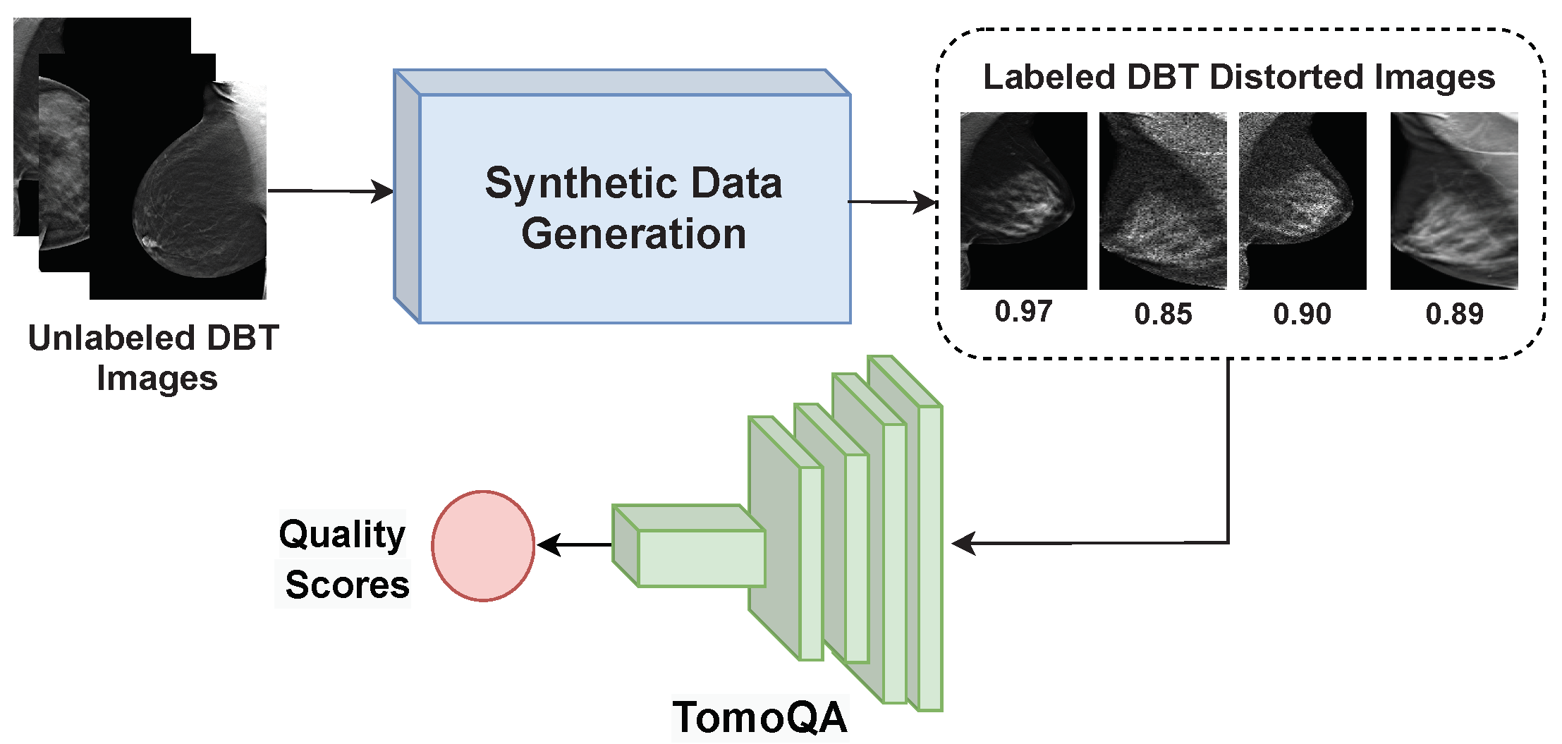
For the DBT quality assessment, we generated distorted images with corresponding objective quality scores following the synthetic data generation strategy discussed in Section 4.1. The detailed distribution of the used DBT quality assessment dataset is shown in

Table 1. Overview of the DBT dataset for quality assessment.

	Train	Test
No. of Patient	40	10
Blurred	40	10
Gamma Correction	80	20
Speckle Noise	40	10
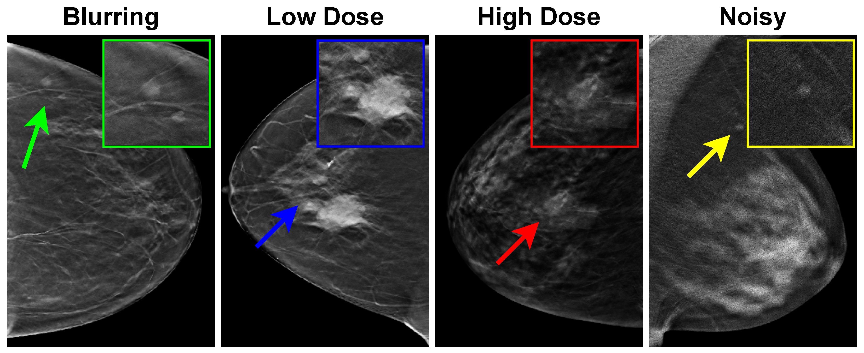
Total Images	200	50

. The DBT images of 50 patients were used to generate the synthetic image quality dataset. We divided the DBT images patient-wise into training and testing sets. It should be noted that we select a single DBT image from each patient randomly. For each image, we generated a blurred image, two images with gamma correction, and a noisy speckle image. Thus, the total number of distorted images is 250.

For breast tumor malignancy prediction, in terms of ROI selection, the tumors are center-cropped and extracted from the annotated DBT image. The selected ROI are then all resized into identical dimensions of $224\times 224$ to fit the input of various radiomics extraction deep learning-based networks. Then, we divide the DBT images and the corresponding patches patient-wise into training and testing sets.

Table 2. Overview of the DBT dataset for tumor malignancy prediction experiments.

	No. of Patients		No. of Tumor Patches		Augmented Patches
	Train	Test	Train	Test	Train	Test
Benign	50	12	114	23	114	23
Malignant	27	12	63	23	126	23
Total	77	24	177	46	240	46

summarizes the DBT dataset used in the breast tumor malignancy prediction task. The dataset is split as follows: approximately $80\%$ for training and $20\%$ for testing (patient-wise). Out of the 223 tumor patches utilized in our study, it was found that 138 cases were categorized as benign, whereas 85 cases were categorized as malignant. This disparity in class distribution creates a significant bias toward the predominant class (benign), resulting in a reduction in the predictive capability of the proposed method and insufficient prediction for the minority class (malignant). It is clear that the number of benign tumors in the training set is approximately twice that of the malignant tumors. To address this challenge, the number of tumor patches in training data increases to balance the dataset, utilizing multiple augmentation processes. We doubled the number of malignant tumor images by jointly flipping all patches in the training set horizontally and vertically. This eventually resulted in 114 benign patches and 126 malignant tumor patches, with a total of 240 tumor patches in the training set. In addition, we used 46 tumor patches for the test consisting of 23 benign patches and 23 malignant patches.

5.2. Evaluation Metrics

We evaluated the proposed breast tumor malignancy prediction method regarding classification accuracy, precision, recall, and F1-score. Accuracy is the most popular metric for evaluating breast cancer screening methods and can be expressed as follows:

$$Accuracy=\frac{TP+TN}{TP+FP+TN+FN}$$

(11)

Precision is the fraction of true positive samples among all positive samples. The recall is referred to as sensitivity and defined as the fraction of true positive instances among all positive classified samples. The F1-score combines precision and recall. It is the harmonic mean of precision and recall. These metrics are computed as follows:

$$\begin{array}{c}\mathrm{precision}=\frac{TP}{TP+FP}\hfill \\ \mathrm{recall}=\frac{TP}{TP+FN}\hfill \\ \mathrm{F}1\text{-}\mathrm{score}=2\times \frac{\mathrm{precision}\times \mathrm{recall}}{\mathrm{precision}+\mathrm{recall}}\hfill \end{array}$$

(12)

where true positive ($TP$) is the number of malignant tumors correctly classified as malignant. True negative ($TN$) represents the number of correctly classified benign tumors. False positive ($FP$) is the number of malignant tumors wrongly classified as benign. False negative ($FN$) stands for the number of benign tumors wrongly classified as malignant.

We evaluate the proposed NR-IQA model–TomoQA in terms of the Pearson linear correlation coefficient (PLCC) [44] and the Spearman rank order correlation coefficient (SROCC) [45]. The comprehensive details of the evaluation process and analysis for the TomoQA model are provided in Appendix A.

5.3. Performance Evaluation of the Proposed Malignancy Prediction Approach

Indeed, the empirical evidence from studies [20,24,26], specifically within the context of tumor feature extraction from DBT images, underscores the commendable performance of AlexNet as a feature extractor. Demonstrating its ability to deliver remarkable results and achieve high classification performance, AlexNet emerges as a promising choice as the baseline model for our task.

To demonstrate the effectiveness of the proposed method,

Table 3. Evaluating the proposed malignancy prediction approach compared with the baseline. The best results are highlighted in bold.

	Backbone	Accuracy (%)	Precision (%)	Recall (%)	F1-Score (%)
Baseline	AlexNet	69.57	65.52	82.61	73.08
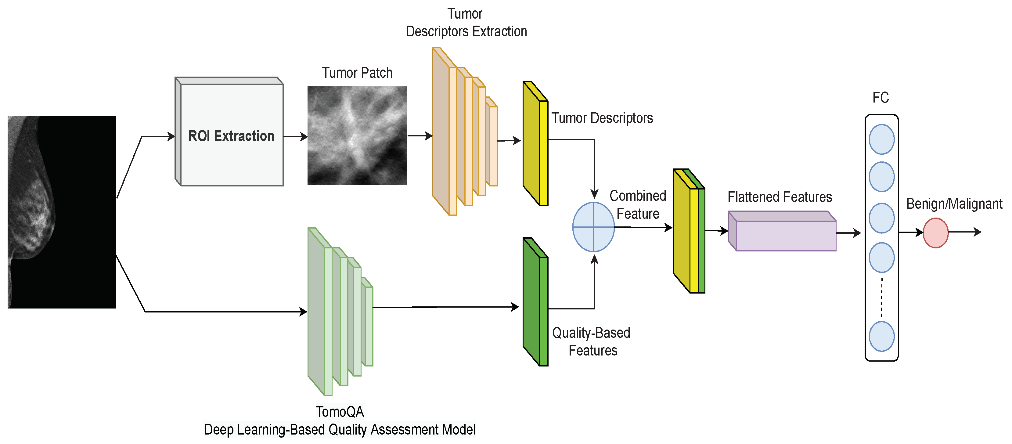
Proposed	AlexNet + TomoQA	78.26	88.24	65.22	75.00

presents results that compare the baseline model, which does not incorporate DBT image quality-aware features, with the proposed quality-aware model. The focus lies on the classification of breast tumors utilizing tumor descriptor features and integrating quality-based features. This comparison serves to highlight the added value and performance enhancements achieved through the incorporation of quality-aware features in our model.

By comparing the baseline model with our proposed quality-aware model, it becomes evident that our novel approach significantly enhances the classification performance across metrics, including accuracy, precision, and F1-score. Notably, our proposed method achieves an impressive accuracy of 78.26%, marking an 8% improvement over the baseline. Moreover, the precision reaches 88.24%, showcasing a remarkable 23% increase compared with the baseline. This substantial gain in precision underscores our model’s proficiency in accurately identifying positive instances. While the baseline achieves a higher true positive rate, our proposed method excels in terms of the F1-score, indicating superior overall performance.

Alternative experiments have been carried out to obtain a more reliable estimate of the model’s performance compared with a single train-test split. We turn to employing the k-fold cross-validation technique. This approach involves randomly dividing the dataset’s images into k groups, or folds, of approximately equal size. The first fold is treated as a validation set, and the model is trained on the remaining $k-1$ folds. It is a resampling procedure that assesses the performance of a predictive model and helps to evaluate how well a model generalizes to unseen data.

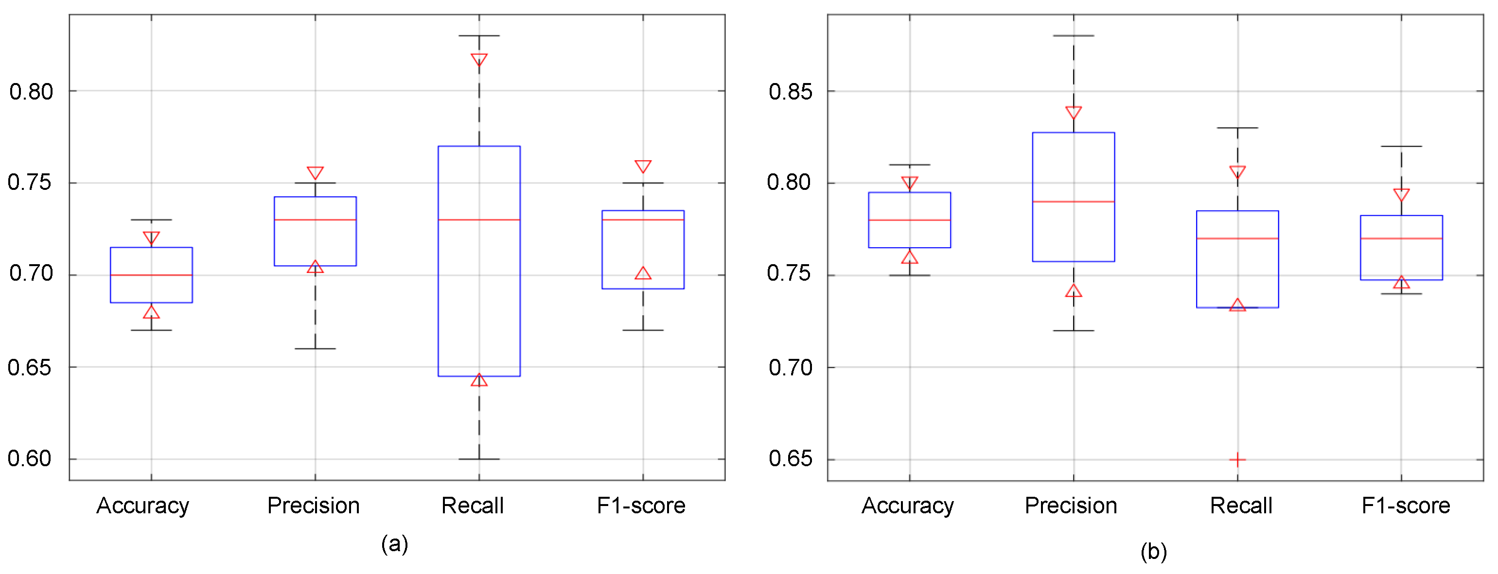
Figure 7 presents boxplots visualizing the distribution of evaluation metrics across the k-fold cross-validation with k = 5 for both the baseline and proposed methods. Each boxplot summarizes the data using a five-number summary: minimum, maximum, first quartile (Q1), median, and third quartile (Q3). The red horizontal line within each box represents the median value, offering a quick comparison of central tendencies between the two methods for each metric.

Notably, it becomes evident that the proposed model surpasses the baseline in terms of accuracy, precision and F1-score across various folds’ validation. As depicted in Figure 7, the minimum, maximum, and median values associated with the proposed model consistently outperform those of the baseline. This is indicative of the proposed model’s superior predictive capacity, as it not only achieves higher accuracy on average but also demonstrates better performance across the validation folds, from the lowest to the highest observed values. Regarding the recall values, while the baseline exhibits a broader distribution, indicating a wider range of performance outcomes, the proposed model demonstrates a more concentrated distribution. Despite the baseline’s higher maximum, the proposed model notably boasts median recall values. This suggests that although the baseline model may exhibit variability in its recall performance, the proposed model consistently achieves superior recall rates.

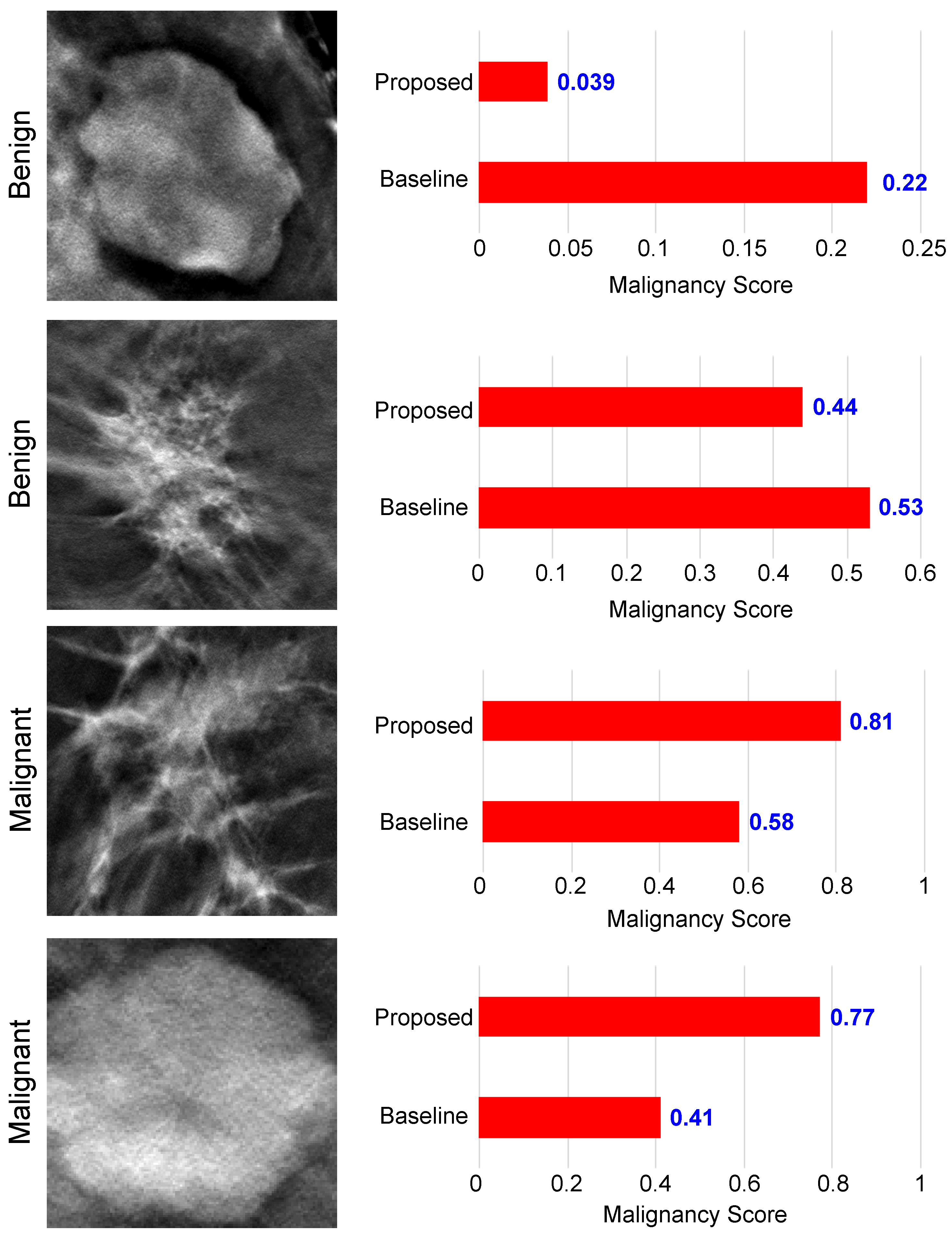
In Figure 8, we present a visual representation of malignancy scores for four DBT images, comprising two benign and two malignant cases. The malignancy score ranges from 0 to 1 and serves as an indicator of tumor carcinogenicity. Benign tumors are characterized by low malignancy scores, closely approaching 0, while the probability of malignant tumors grows as the malignancy score reaches 1.

As we can see from Figure 8, in the context of benign tumors, both the baseline and our proposed model demonstrated accurate classification for the upper image. However, the proposed method achieved a lower malignancy score of 0.039 compared with the baseline. Turning attention to the lower image, which shares a shape similarity with malignant tumors, the proposed model obtained a score of 0.44 < 0.5, correctly classifying the tumor. In contrast, the baseline model made an incorrect classification, assigning a score of 0.53 > 0.5. Similar results can be observed when examining the results of malignant tumor images. We see that the proposed method was able to obtain a high malignancy score for both images, with a score of 0.81 and 0.77, superior to the basic model. Also, the basic model obtained incorrect results for the lower image, which is similar in appearance to benign tumors. This analysis underscores the improved classification capability of our proposed model, particularly in scenarios with borderline malignancy scores, enhancing its precision in distinguishing between benign and malignant tumor patterns.

Table 4. Comparing the performance of the proposed method with existing breast tumor classification methods. The best results are highlighted in bold.

Method	Backbone Model	Accuracy (%)	Precision (%)	Recall (%)	F1-Score (%)
Yeh et al. [19]	LeNet	59.11	87.50	66.67	75.00
Ricciardi et al. [20]	DBT-DCNN	64.54	73.90	65.42	69.39
Doganay et al. [25]	Vgg16	65.57	73.08	82.60	77.56
Samala et al. [26]	AlexNet	74.66	78.95	78.95	79.00
Moghadam et al. [22]	ML approach	80.67	75.11	77.12	76.10
Proposed	AlexNet + TomoQA	78.26	88.24	65.22	75.00

compares the proposed malignancy prediction method with existing breast tumor classification methods for DBT images. To conduct a fair comparative study, we trained and tested all methods using the same training and testing DBT datasets.

Table 4 demonstrates that the performance of the proposed method outperforms all other compared methods in terms of accuracy and precision. Thanks to the proposed dual-branch approach, quality-aware features help the classifier focus its attention on the most relevant regions of the image and provide complementary information to the tumor descriptor branch that discerns meaningful patterns associated with the tumor, improving classification accuracy.

As we can see, the proposed method outperforms the method presented in [26] which achieved a competitive performance over the other deep learning-based methods, with an accuracy of 75% and an F1-score of 79%. Following [26], we used the INbreast mammogram dataset [46] to fine-tune the AlexNet model in the first stage of the method, and then we used the DBTex train set to further fine-tune the model. A potential drawback of [26] is the requirement for a mammography dataset, which may not always be accessible for training in the initial stage of the method. Additionally, the methodology proposed in the study [22] demonstrated commendable performance, achieving competitiveness with an accuracy of 80.67% and specificity of 77.12%. However, it is crucial to mention a significant aspect of the classic machine learning technique of Moghadam et al. [22]—it relies heavily on hand-crafted features tailored to a specific dataset. Although they stated in their study that the use of 15 selected features represented the optimum point via trial and error, they did not specify what these features are and how they extracted them, which raises a reproducibility limitation, along with the inherent limitations, as the effectiveness of selected features cannot be guaranteed to achieve the same level of performance when applied to diverse digital DBT datasets. Furthermore, it does not operate as an end-to-end system. Instead, this method involves a series of seven intricate sequential steps, unlike deep learning methods.

5.4. Ablation Study

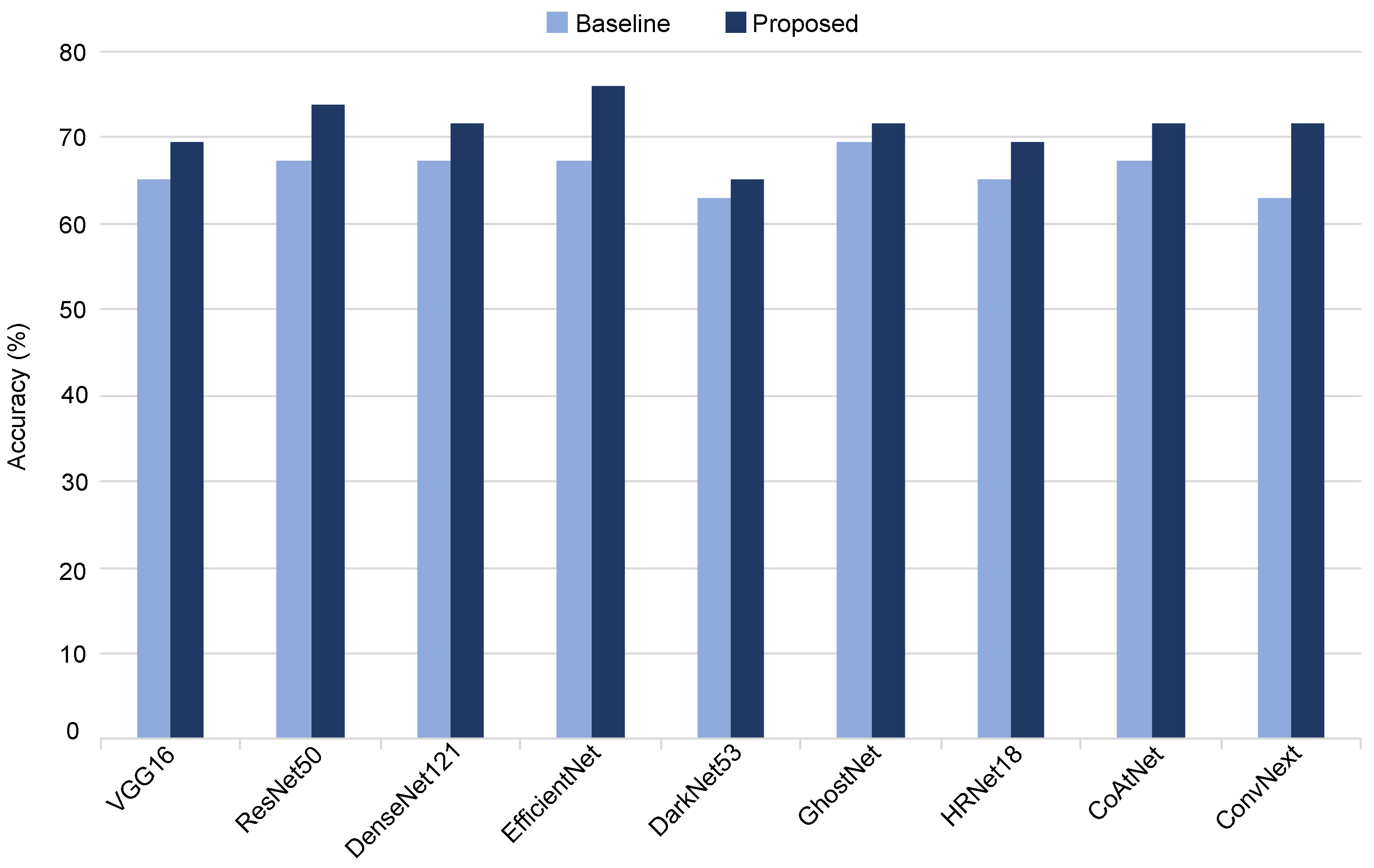
To demonstrate the efficacy of our proposed method, we conducted a comprehensive evaluation by applying the quality-aware framework to various CNN-based classification networks, including VGG16, ResNet50, DensNet121, EfficientNet, DarkNet53, GhostNet, HRNet, CoAtNet, and ConvNext. The performance of each model, when employed with our quality-aware approach, was compared against its respective baseline in terms of accuracy.

The outcomes illustrated in Figure 9 reveal notable improvements across all evaluated classification models. Specifically, the proposed method enhances the classification accuracy of ResNet50, EfficientNet, and ConvNext by 6%, 9%, and 9%, respectively, underscoring the broad applicability and consistent performance gains achieved by our quality-aware approach across diverse CNN architectures.

Statistical analysis: As shown above, the performance attained by the proposed method surpasses those of the baseline models (VGG16, ResNet50, DensNet121, EfficientNet, DarkNet53, GhostNet, HRNet, CoAtNet, and ConvNext), underscoring its efficacy in enhancing the classification outcomes across all evaluated models. In this study, we employed McNemar’s statistical test to ascertain the statistical significance of the performance disparities concerning accuracy between the proposed method and different baseline models. McNemar’s test is specifically designed for comparing paired nominal data, which makes it suitable for comparing the performance of two classifiers in a binary classification setting. In particular, we employed the continuity-corrected version of McNemar’s test, which is the more commonly used variant. A continuity-corrected version of McNemar’s test is governed by the following equation:

$${\chi }^2=\frac{{\left(\right|B-C|-1)}^2}{(B+C)}$$

(13)

where B denotes the count of instances correctly predicted by the baseline but incorrectly by the proposed method. C signifies the count of instances correctly predicted by the proposed method but incorrectly by the baseline. The $(-1)$ in the numerator is included to adjust for the continuity correction. Once we have calculated McNemar’s statistic, we can compare it with the chi-squared distribution with 1 degree of freedom to obtain the p-value. This p-value indicates the probability of observing the discrepancy between the two models by chance alone.

Table 5. Comparison between the proposed method and baseline in terms of the accuracy (statistically significant differences are shown in bold).

Proposec vs. Baseline	Best Accuracy Achieved (%) by the Proposed Method	Best Accuracy Achieved (%) by the Baseline	p-Value
AlexNet	78.26	69.57	<0.003
VGG16	69.57	65.22	<0.05
ResNet50	73.91	67.39	<0.05
DenseNet121	71.74	67.39	<0.02
EfficientNet	76.08	67.39	<0.007
DarkNet53	65.22	63.04	<0.05
GhostNet	71.74	69.57	<0.009
HRNet18	69.57	65.22	<0.05
CoAtNet	71.74	67.39	<0.02
ConvNext	71.74	63.04	<0.03

shows the statistical analysis of the accuracy values of the proposed model and each baseline model. In this table, a p-value lower than $0.05$ indicates statistical significance. As can be seen in Table 5, for each baseline model, the results of the proposed method are more statistically significant than the ones of the baseline model.

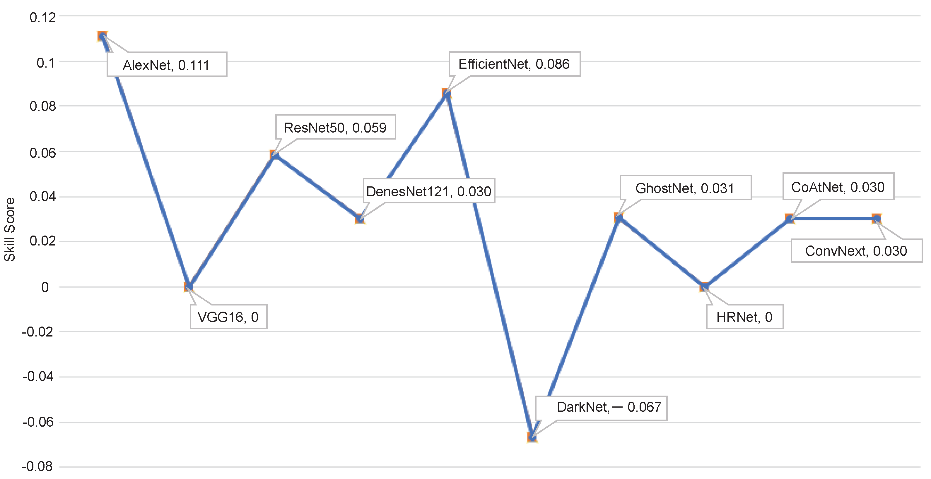
Figure 10 shows the skill score ($SS$) of different variants of the proposed approach. $SS$ measures the accuracy improvement of a model regarding the accuracy of a reference model. $SS$ can be expressed as follows:

$$SS=1-\frac{M_{Ref}}{M_{Ev}}$$

(14)

where $M_{Ref}$ and $M_{Ev}$ stand for the accuracy of the reference and evaluated models, respectively. As the baseline AlexNet model obtained the highest classification accuracy, we used it as a reference model. As shown, the proposed method based on the AlexNet model achieves the highest skill score.

5.5. Analyzing the Computational Efficiency of the Proposed Method

Furthermore, to address concerns regarding computational efficiency, we present an additional analysis in Figure 11 which highlights the accuracy improvement ratio (AIR), i.e., how the proposed method increased the accuracy of all models over the models’ baseline compared with the number of trainable parameters that indicate the computational complexity for each evaluated model. As shown, there is a noticeable variation in complexity between the evaluated models. We can see that EfficientNet, GhostNet, and CoAtNet have a few numbers of trainable parameters ranging from 2 to 9 million parameters with an accuracy improvement rate of $11\%$, $3\%$, and $7\%$, at a variance from DenseNet121 and ConvNext which contained up to 90 million parameters with an accuracy improvement rate of $6\%$ and $12\%$. VGG16 and HRNet have an acceptable number of trainable parameters (<40 million) and obtained significant accuracy improvement with a rate of $18\%$. However, considering that the obtained accuracy of AlexNet ($78\%$) and the high accuracy improvement ratio ($11\%$) with a high computational efficiency resulting from the ability to train a small number of parameters (<10 million) leads to lower resource requirements and faster inference, we can infer that using AlexNet for extracting tumor descriptors in the proposed method is an excellent choice.

5.6. Enhancing Classification Accuracy through Ensemble Models

Aggregating multiple deep learning models can significantly enhance classification accuracy by leveraging the diversity and complementary strengths of individual models. This ensemble approach aims to mitigate the weaknesses of individual models and capitalize on their collective predictive power. By combining the predictions of diverse models, the ensemble can capture a broader range of patterns and features in the data, leading to a more robust and accurate classification performance.

Based on results shown in Section 5.3 and Section 5.4, we select the top-performing breast tumor malignancy prediction models in terms of accuracy, precision, and F1-score (AlexNet, ResNet50, EfficientNet, GhostNet, CoAtNet, and DensNet121). To construct the ensemble classification approach, we aggregate the malignancy scores of the top-performing models using the average and median aggregation functions.

As presented in

Table 6. Evaluating different aggregation-based ensemble models. The best results are highlighted in bold.

	Accuracy (%)	Precision (%)	Recall (%)	F1-Score (%)
Average Aggregation	84.78	90.11	82.61	82.61
Median Aggregation	86.96	90.48	82.61	86.36

, the average aggregation for ensembled models achieves an accuracy of $84.78\%$, better than the individual proposed AlexNet-based quality-aware method with a $6\%$ enhancement. Although the mean aggregation function yields an acceptable performance, the median aggregation leads to slightly better results. For ensembled models, we obtain an accuracy of $86.96\%$, $90.48\%$ precision, and an F1-score of $86.36\%$.

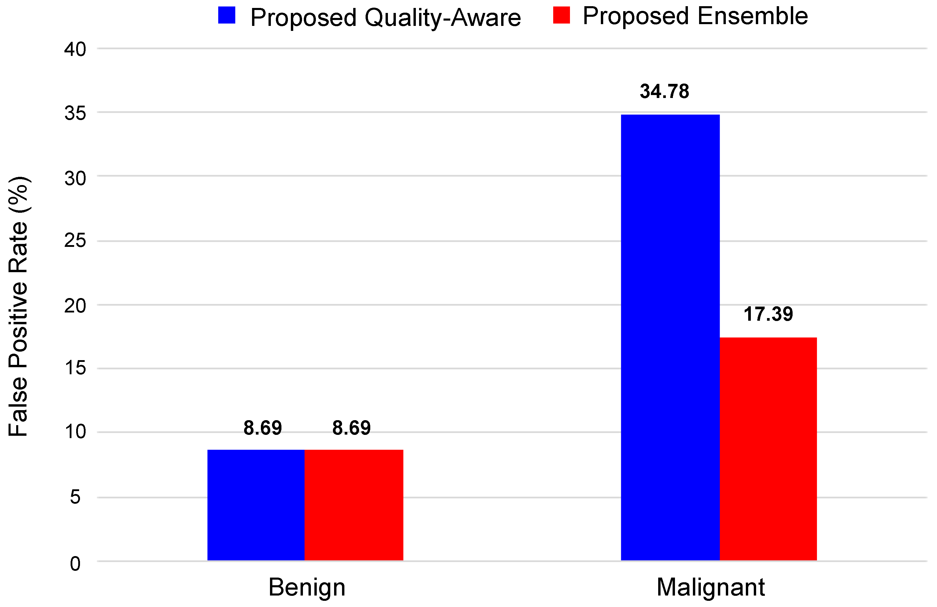
Figure 12 shows the false positive rate (FPR) for the proposed method and the best-proposed ensemble method (ensemble models, based on the median aggregation function). Here, we can see that both methods efficiently classify the benign tumors of the DBT image with an accuracy of $91.3\%$. In the case of malignant tumors, ensemble models with the median aggregation function achieved a higher classification accuracy of $82.60\%$, which is $17\%$ better than the AlexNet-based classification method.

Based on the analysis presented here and in Section 5.3, Section 5.4, Section 5.5 and Section 5.6, it is clear that the use of the quality-aware features can significantly enhance breast tumor classification on DBT images, and the proposed ensemble approach can achieve accurate malignancy prediction while outperforming the state-of-the-art methods.

5.7. Evaluating the Proposed Method on the Breast Mammography Modality

To further validate the effectiveness of our proposed quality-aware tumor classification approach and ensure its generalizability across different datasets, we conducted evaluations using an alternative breast imaging modality, namely breast mammography. Since there are no other publicly available DBT datasets, our assessment focused on the performance of the proposed method using the INbreast dataset [46]. Comprising 410 images from 115 women, INbreast serves as a valuable resource for research in mammogram-based breast cancer diagnosis. It has been used in several studies in the development and evaluation of methodologies for breast tumor classification.

By following the implementation of our proposed pipeline, we split the dataset as follows: about $80\%$ for training and $20\%$ for testing (randomly). It is worth noting that we did not retrain the TomoQA model using mammogram images. Instead, we leveraged the same model previously trained on DBT images due to the similarities between mammogram images and 2D DBT slices.

Table 7. Evaluating the proposed malignancy prediction approach compared with the baseline for Inbreast Dataset. The best results are highlighted in bold.

	Backbone	Accuracy (%)	Precision (%)	Recall (%)	F1-Score (%)
Baseline	AlexNet	77.1	81.8	87.9	84.7
Proposed	AlexNet + TomoQA	85.0	84.1	90.0	86.9

highlights the clear advantage of our quality-aware model compared with the baseline model lacking image quality-aware features. By comparing their performance across all metrics, we see a significant enhancement in classification achieved by our method. We can see that the proposed method improves the accuracy by $8\%$ over the baseline with an enhancement of approximability of $3\%$ for each of the precision, recall, and F1-score metrics.

6. Conclusions

In this paper, we have proposed a deep learning-based quality-aware approach for breast tumor malignancy prediction in digital breast tomosynthesis images. The proposed approach has two main components: an NR-IQA model we called TomoQA for extracting DBT image quality-based features and a deep learning network for extracting tumor descriptors from the tumor region. Both tumor descriptors and quality-based features are integrated to classify breast tumors as benign or malignant. Experimental results demonstrated that the proposed method surpassed the baseline models (classification without employing quality-based features) by $9\%$ in terms of accuracy. This indicates that the proposed approach could extract discriminative tumor descriptors from digital breast tomosynthesis images that improve malignancy prediction accuracy. Moreover, combining the high-performance evaluated models led to a classification accuracy of $86.96\%$.

In future work, we aim to delve deeper into refining our methodology. Specifically, our focus will shift toward exploring different pooling techniques to effectively fuse features extracted from various DBT slices to further improve the classification accuracy. Additionally, we will investigate the integration of multimodal data (e.g., DBT, mammography, MRI, and clinical data) for improved analysis. Moreover, we will explore the utilization of advanced machine learning techniques, such as transfer learning and federated learning, to develop a robust breast tumor classification model in DBT images.

References

1. Jemal, A.; Siegel, R.; Ward, E.; Hao, Y.; Xu, J.; Murray, T.; Thun, M.J. Cancer Statistics, 2008. CA Cancer J. Clin. 2008, 58, 71–96. [Google Scholar] [CrossRef]
2. Mridha, M.F.; Hamid, M.A.; Monowar, M.M.; Keya, A.J.; Ohi, A.Q.; Islam, M.R.; Kim, J.M. A Comprehensive Survey on Deep-Learning-Based Breast Cancer Diagnosis. Cancers 2021, 13, 6116. [Google Scholar] [CrossRef] [PubMed]
3. Jasti, V.D.P.; Zamani, A.S.; Arumugam, K.; Naved, M.; Pallathadka, H.; Sammy, F.; Raghuvanshi, A.; Kaliyaperumal, K. Computational Technique Based on Machine Learning and Image Processing for Medical Image Analysis of Breast Cancer Diagnosis. Secur. Commun. Netw. 2022, 2022, 1918379. [Google Scholar] [CrossRef]
4. Guy, C.; Ffytche, D. An Introduction to the Principles of Medical Imaging; World Scientific Publishing Co.: Singapore, 2005. [Google Scholar] [CrossRef]
5. Iranmakani, S.; Mortezazadeh, T.; Sajadian, F.; Ghaziani, M.F.; Ghafari, A.; Khezerloo, D.; Musa, A.E. A review of various modalities in breast imaging: Technical aspects and clinical outcomes. Egypt. J. Radiol. Nucl. Med. 2020, 51, 57. [Google Scholar] [CrossRef]
6. Heywang-Köbrunner, S.H.; Hacker, A.; Sedlacek, S. Advantages and Disadvantages of Mammography Screening. Breast Care 2011, 6, 2. [Google Scholar] [CrossRef] [PubMed]
7. Dhamija, E.; Gulati, M.; Deo, S.V.S.; Gogia, A.; Hari, S. Digital Breast Tomosynthesis: An Overview. Indian J. Surg. Oncol. 2021, 12, 315–329. [Google Scholar] [CrossRef]
8. Helvie, M.A. Digital Mammography Imaging: Breast Tomosynthesis and Advanced Applications. Radiol. Clin. N. Am. 2010, 48, 917–929. [Google Scholar] [CrossRef] [PubMed]
9. Haas, B.M.; Kalra, V.; Geisel, J.; Raghu, M.; Durand, M.; Philpotts, L.E. Comparison of Tomosynthesis Plus Digital Mammography and Digital Mammography Alone for Breast Cancer Screening. Radiology 2013, 269, 694–700. [Google Scholar] [CrossRef]
10. Jalalian, A.; Mashohor, S.; Mahmud, R.; Karasfi, B.; Saripan, M.I.B.; Ramli, A.R.B. Foundation and methodologies in computer-aided diagnosis systems for breast cancer detection. EXCLI J. 2017, 16, 113–137. [Google Scholar] [CrossRef]
11. Amrane, M.; Oukid, S.; Gagaoua, I.; Ensari, T. Breast cancer classification using machine learning. In Proceedings of the 2018 Electric Electronics, Computer Science, Biomedical Engineerings’ Meeting (EBBT), Istanbul, Turkey, 8–19 April 2018; IEEE: Piscataway, NJ, USA, 2018; pp. 1–4. [Google Scholar] [CrossRef]
12. Omondiagbe, D.A.; Veeramani, S.; Sidhu, A.S. Machine Learning Classification Techniques for Breast Cancer Diagnosis. IOP Conf. Ser. Mater. Sci. Eng. 2019, 495, 012033. [Google Scholar] [CrossRef]
13. Li, H.; Chen, D.; Nailon, W.H.; Davies, M.E.; Laurenson, D.I. Dual Convolutional Neural Networks for Breast Mass Segmentation and Diagnosis in Mammography. IEEE Trans. Med. Imaging 2022, 41, 3–13. [Google Scholar] [CrossRef]
14. El-Shazli, A.M.A.; Youssef, S.M.; Soliman, A.H. Intelligent Computer-Aided Model for Efficient Diagnosis of Digital Breast Tomosynthesis 3D Imaging Using Deep Learning. Appl. Sci. 2022, 12, 5736. [Google Scholar] [CrossRef]
15. Bai, J.; Posner, R.; Wang, T.; Yang, C.; Nabavi, S. Applying deep learning in digital breast tomosynthesis for automatic breast cancer detection: A review. Med. Image Anal. 2021, 71, 102049. [Google Scholar] [CrossRef] [PubMed]
16. Debelee, T.G.; Schwenker, F.; Ibenthal, A.; Yohannes, D. Survey of deep learning in breast cancer image analysis. Evol. Syst. 2019, 11, 143–163. [Google Scholar] [CrossRef]
17. Pinto, M.C.; Rodriguez-Ruiz, A.; Pedersen, K.; Hofvind, S.; Wicklein, J.; Kappler, S.; Mann, R.M.; Sechopoulos, I. Impact of Artificial Intelligence Decision Support Using Deep Learning on Breast Cancer Screening Interpretation with Single-View Wide-Angle Digital Breast Tomosynthesis. Radiology 2021, 300, 529–536. [Google Scholar] [CrossRef]
18. Geiser, W.R.; Einstein, S.A.; Yang, W.T. Artifacts in Digital Breast Tomosynthesis. Am. J. Roentgenol. 2018, 211, 926–932. [Google Scholar] [CrossRef]
19. Yeh, J.Y.; Chan, S. CNN-Based CAD for Breast Cancer Classification in Digital Breast Tomosynthesis. In Proceedings of the 2nd International Conference on Graphics and Signal Processing—ICGSP18, Sydney, Australia, 6–8 October 2018; ACM Press: New York, NY, USA, 2018; pp. 26–30. [Google Scholar] [CrossRef]
20. Ricciardi, R.; Mettivier, G.; Staffa, M.; Sarno, A.; Acampora, G.; Minelli, S.; Santoro, A.; Antignani, E.; Orientale, A.; Pilotti, I.; et al. A deep learning classifier for digital breast tomosynthesis. Phys. Med. 2021, 83, 184–193. [Google Scholar] [CrossRef]
21. Lee, W.; Lee, H.; Lee, H.; Park, E.K.; Nam, H.; Kooi, T. Transformer-based Deep Neural Network for Breast Cancer Classification on Digital Breast Tomosynthesis Images. Radiol. Artif. Intell. 2023, 5, e220159. [Google Scholar] [CrossRef]
22. Moghadam, F.S.; Rashidi, S. Classification of benign and malignant tumors in Digital Breast Tomosynthesis images using Radiomic-based methods. In Proceedings of the 2023 13th International Conference on Computer and Knowledge Engineering (ICCKE), Mashhad, Iran, 1–2 November 2023; IEEE: Piscataway, NJ, USA, 2023; pp. 203–208. [Google Scholar] [CrossRef]
23. SPIE-AAPM-NCI DAIR Digital Breast Tomosynthesis Lesion Detection Challenge. Available online: https://www.aapm.org/GrandChallenge/DBTex2/ (accessed on 24 January 2023).
24. Zhang, Y.; Wang, X.; Blanton, H.; Liang, G.; Xing, X.; Jacobs, N. 2D Convolutional Neural Networks for 3D Digital Breast Tomosynthesis Classification. In Proceedings of the 2019 IEEE International Conference on Bioinformatics and Biomedicine (BIBM), San Diego, CA, USA, 18–21 November 2019; IEEE: Piscataway, NJ, USA, 2019; pp. 1013–1017. [Google Scholar] [CrossRef]
25. Doganay, E.; Li, P.; Luo, Y.; Chai, R.; Guo, Y.; Wu, S. Breast cancer classification from digital breast tomosynthesis using 3D multi-subvolume approach. In Proceedings of the Medical Imaging 2020: Imaging Informatics for Healthcare, Research, and Applications, Houston, TX, USA, 16–17 February 2020; SPIE: Wallisellen, Switzerland, 2020; Volume 11318, p. 113180D. [Google Scholar] [CrossRef]
26. Samala, R.K.; Chan, H.P.; Hadjiiski, L.; Helvie, M.A.; Richter, C.D.; Cha, K.H. Breast Cancer Diagnosis in Digital Breast Tomosynthesis: Effects of Training Sample Size on Multi-Stage Transfer Learning Using Deep Neural Nets. IEEE Trans. Med. Imaging 2019, 38, 686–696. [Google Scholar] [CrossRef]
27. Domenec, P. Lesion Detection in Breast Tomosynthesis Using Efficient Deep Learning and Data Augmentation Techniques. In Artificial Intelligence Research and Development, Proceedings of the 23rd International Conference of the Catalan Association for Artificial Intelligence, Online, 20–22 October 2021; IOS Press: Amsterdam, The Netherlands, 2021; Volume 339, p. 315. [Google Scholar]
28. Krizhevsky, A.; Sutskever, I.; Hinton, G.E. ImageNet classification with deep convolutional neural networks. Commun. ACM 2012, 60, 84–90. [Google Scholar] [CrossRef]
29. Liu, S.; Deng, W. Very deep convolutional neural network based image classification using small training sample size. In Proceedings of the 2015 3rd IAPR Asian Conference on Pattern Recognition (ACPR), Kuala Lumpur, Malaysia, 3–6 November 2015; IEEE: Piscataway, NJ, USA, 2015; pp. 730–734. [Google Scholar] [CrossRef]
30. He, K.; Zhang, X.; Ren, S.; Sun, J. Deep Residual Learning for Image Recognition. In Proceedings of the 2016 IEEE Conference on Computer Vision and Pattern Recognition (CVPR), Las Vegas, NV, USA, 27–30 June 2016; IEEE: Piscataway, NJ, USA, 2016; pp. 770–778. [Google Scholar] [CrossRef]
31. Huang, G.; Liu, Z.; Maaten, L.V.D.; Weinberger, K.Q. Densely Connected Convolutional Networks. In Proceedings of the 2017 IEEE Conference on Computer Vision and Pattern Recognition (CVPR), Honolulu, HI, USA, 21–26 July 2017; IEEE: Piscataway, NJ, USA, 2017; pp. 2261–2269. [Google Scholar] [CrossRef]
32. Tan, M.; Le, Q. EfficientNet: Rethinking Model Scaling for Convolutional Neural Networks. In Proceedings of the 36th International Conference on Machine Learning, PMLR, Long Beach, CA, USA, 9–15 June 2019; Volume 97, pp. 6105–6114. [Google Scholar] [CrossRef]
33. Redmon, J.; Farhadi, A. YOLOv3: An Incremental Improvement. arXiv 2018, arXiv:1804.02767. [Google Scholar] [CrossRef]
34. Han, K.; Wang, Y.; Tian, Q.; Guo, J.; Xu, C.; Xu, C. GhostNet: More Features From Cheap Operations. In Proceedings of the 2020 IEEE/CVF Conference on Computer Vision and Pattern Recognition (CVPR), Seattle, WA, USA, 13–19 June 2020; IEEE: Piscataway, NJ, USA, 2020; pp. 1577–1586. [Google Scholar] [CrossRef]
35. Wang, J.; Sun, K.; Cheng, T.; Jiang, B.; Deng, C.; Zhao, Y.; Liu, D.; Mu, Y.; Tan, M.; Wang, X.; et al. Deep High-Resolution Representation Learning for Visual Recognition. IEEE Trans. Pattern Anal. Mach. Intell. 2021, 43, 3349–3364. [Google Scholar] [CrossRef] [PubMed]
36. Dai, Z.; Liu, H.; Le, Q.V.; Tan, M. CoAtNet: Marrying Convolution and Attention for All Data Sizes. Adv. Neural Inf. Process. Syst. 2021, 34, 3965–3977. [Google Scholar] [CrossRef]
37. Liu, Z.; Mao, H.; Wu, C.Y.; Feichtenhofer, C.; Darrell, T.; Xie, S. A ConvNet for the 2020s. In Proceedings of the 2022 IEEE/CVF Conference on Computer Vision and Pattern Recognition (CVPR), New Orleans, LA, USA, 18–24 June 2022; pp. 11966–11976. [Google Scholar] [CrossRef]
38. Hendrycks, D.; Gimpel, K. Gaussian Error Linear Units (GELUs). arXiv 2016, arXiv:1606.08415. [Google Scholar] [CrossRef]
39. Tirada, N.; Li, G.; Dreizin, D.; Robinson, L.; Khorjekar, G.; Dromi, S.; Ernst, T. Digital Breast Tomosynthesis: Physics, Artifacts, and Quality Control Considerations. RadioGraphics 2019, 39, 413–426. [Google Scholar] [CrossRef]
40. Gao, Q.; Li, S.; Zhu, M.; Li, D.; Bian, Z.; Lyu, Q.; Zeng, D.; Ma, J. Blind CT Image Quality Assessment via Deep Learning Framework. In Proceedings of the 2019 IEEE Nuclear Science Symposium and Medical Imaging Conference (NSS/MIC), Manchester, UK, 26 October–2 November 2019; IEEE: Piscataway, NJ, USA, 2019; pp. 1–4. [Google Scholar] [CrossRef]
41. Gao, Q.; Li, S.; Zhu, M.; Li, D.; Bian, Z.; Lv, Q.; Zeng, D.; Ma, J. Combined global and local information for blind CT image quality assessment via deep learning. In Proceedings of the Medical Imaging 2020: Image Perception, Observer Performance, and Technology Assessment, Houston, TX, USA, 15–20 February 2020; SPIE: Wallisellen, Switzerland, 2020; Volume 11316, p. 1131615. [Google Scholar] [CrossRef]
42. Baig, M.A.; Moinuddin, A.A.; Khan, E. PSNR of Highest Distortion Region: An Effective Image Quality Assessment Method. In Proceedings of the 2019 International Conference on Electrical, Electronics and Computer Engineering (UPCON), Aligarh, India, 8–10 November 2019; pp. 1–4. [Google Scholar] [CrossRef]
43. Wang, Z.; Bovik, A.; Sheikh, H.; Simoncelli, E. Image Quality Assessment: From Error Visibility to Structural Similarity. IEEE Trans. Image Process. 2004, 13, 600–612. [Google Scholar] [CrossRef]
44. Song, P.X.-K. Correlated Data Analysis: Modeling, Analytics, and Applications, 1st ed.; Springer: New York, NY, USA, 2007. [Google Scholar] [CrossRef]
45. Gautheir, T.D. Detecting Trends Using Spearman’s Rank Correlation Coefficient. Environ. Forensics 2001, 2, 359–362. [Google Scholar] [CrossRef]
46. Moreira, I.C.; Amaral, I.; Domingues, I.; Cardoso, A.; Cardoso, M.J.; Cardoso, J.S. INbreast: Toward a full-field digital mammographic database. Acad. Radiol. 2012, 19, 236–248. [Google Scholar] [CrossRef]
47. Bosse, S.; Maniry, D.; Wiegand, T.; Samek, W. A deep neural network for image quality assessment. In Proceedings of the 2016 IEEE International Conference on Image Processing (ICIP), Phoenix, AZ, USA, 25–28 September 2016; IEEE: Piscataway, NJ, USA, 2016; pp. 3773–3777. [Google Scholar] [CrossRef]
48. Su, S.; Yan, Q.; Zhu, Y.; Zhang, C.; Ge, X.; Sun, J.; Zhang, Y. Blindly Assess Image Quality in the Wild Guided by a Self-Adaptive Hyper Network. In Proceedings of the 2020 IEEE/CVF Conference on Computer Vision and Pattern Recognition (CVPR), Seattle, WA, USA, 13–19 June 2020; IEEE: Piscataway, NJ, USA, 2020; pp. 3664–3673. [Google Scholar] [CrossRef]
Figure 1. Examples of artifacts affecting DBT images. Blurring, low dose, high dose, and noise manifested as bright or dark pixels are indicated by corresponding green, blue, red, and yellow arrows and boxes, respectively.
Make 06 00029 g001
Figure 2. Proposed framework for breast tumor classification in DBT images.
Make 06 00029 g002
Figure 3. The framework of the proposed DBT image NR-IQA method.
Make 06 00029 g003
Figure 4. The architecture of ConvNext.
Make 06 00029 g004
Figure 5. The architecture of the ConvNext block.
Make 06 00029 g005
Figure 6. Examples of distorted DBT images with the corresponding PSNR, SSIM, and corresponding quality scores.
Make 06 00029 g006
Figure 7. Boxplots of the k-fold cross-validation results with k = 5 for (a) baseline and (b) proposed method.
Make 06 00029 g007
Figure 8. Examples of malignancy score prediction using the proposed method.
Make 06 00029 g008
Figure 9. Evaluating different variations of the proposed malignancy prediction approach.
Make 06 00029 g009
Figure 10. Skill scores of the malignancy prediction models.
Make 06 00029 g010
Figure 11. Accuracy improvement versus the number of trainable parameters of each evaluated model.
Make 06 00029 g011
Figure 12. False positive rate for proposed method and proposed ensemble.
Make 06 00029 g012