Review

GAN-Based Tabular Data Generator for Constructing Synopsis in Approximate Query Processing: Challenges and Solutions

by
Mohammadali Fallahian
*,
Mohsen Dorodchi
and
Kyle Kreth
Department of Computer Science, University of North Carolina at Charlotte, Charlotte, NC 28223, USA
*
Author to whom correspondence should be addressed.
Mach. Learn. Knowl. Extr. 2024, 6(1), 171-198; https://doi.org/10.3390/make6010010
Submission received: 10 November 2023 / Revised: 29 December 2023 / Accepted: 13 January 2024 / Published: 16 January 2024
(This article belongs to the Section Data)

Abstract

:
In data-driven systems, data exploration is imperative for making real-time decisions. However, big data are stored in massive databases that are difficult to retrieve. Approximate Query Processing (AQP) is a technique for providing approximate answers to aggregate queries based on a summary of the data (synopsis) that closely replicates the behavior of the actual data; this can be useful when an approximate answer to queries is acceptable in a fraction of the real execution time. This study explores the novel utilization of a Generative Adversarial Network (GAN) for the generation of tabular data that can be employed in AQP for synopsis construction. We thoroughly investigate the unique challenges posed by the synopsis construction process, including maintaining data distribution characteristics, handling bounded continuous and categorical data, and preserving semantic relationships, and we then introduce the advancement of tabular GAN architectures that overcome these challenges. Furthermore, we propose and validate a suite of statistical metrics tailored for assessing the reliability of GAN-generated synopses. Our findings demonstrate that advanced GAN variations exhibit a promising capacity to generate high-fidelity synopses, potentially transforming the efficiency and effectiveness of AQP in data-driven systems.

1. Introduction

Research and business today rely heavily on big data and their analysis. However, big data are stored in massive databases that make them difficult to retrieve, analyze, share, and visualize using standard database query tools [1]. For data-driven systems, data exploration is imperative for making real-time decisions and understanding the knowledge contained in the data. However, supporting these systems can be costly, especially regarding big data. One of the most critical challenges posed by big data is the high computational cost associated with data exploration and real-time query processing [2]. To assist with the analysis of big data, several systems have been developed, such as Apache Hive, which typically takes a considerable amount of time to respond to analytical queries [3]. However, approximate results can sometimes be provided for a query in a fraction of the execution time in order to resolve this issue, particularly for aggregation queries. This is because aggregation queries are typically designed to provide a big picture for a large amount of information without having to compute an exact answer [4]. The majority of analytical queries require aggregate answers (such as sum(), avg(), count(), min(), and max()) for a given set of queries (joined or nested queries) over one or more categories (grouped by columns) on a subset (where and the existence of) for big data. Approximate Query Processing (AQP) comes to the rescue by identifying a summary of the population (also known as a synopsis) for discovering trends and aggregate functions [5]. Online aggregations and offline precomputed synopses are the two primary categories that can be used to classify existing AQP approaches. Offline techniques summarize the data distribution and return the approximate results by running queries on these synopses. However, online aggregation techniques progressively generate synopses and return approximate results while data are processing. The traditional approach for both categories uses data distribution to generate a subset of data via statistical methods such as sampling methods [2]. One novel technique for AQP is to take advantage of machine learning to further reduce the execution time, improve accuracy, and support all types of aggregate functions. For instance, the DBEst Query processing engine [6] trains models, notably regression models and density estimators, that provide accurate, efficient, and cost-effective responses to different types of aggregate queries. Learning-based AQP (LAQP) [7] and ML-AQP [8] methods build machine learning models based on historically executed queries. The former builds an error model to predict each incoming query’s sampling-based estimation error, whereas the latter trains models that learn patterns to predict future query results with a bound error by applying prediction intervals constructed using Quantile Regression models. Deep Generative Models (DGMs) are instrumental for approximating complex, high-dimensional probability distributions of data populations [9]. By estimating the probability of each observation, DGMs facilitate the generation of data synopses that faithfully represent underlying distributions. Thirumuruganathan et al. [10] have leveraged DGMs for Approximate Query Processing (AQP) using Variational Autoencoder (VAE). VAE [11] generates new data by encoding input distributions into an interpretable latent space wherein auto-encoders recreate the data. Our study introduces a novel approach by employing the Generative Adversarial Network (GAN), another state-of-the-art algorithm, for AQP. Unlike VAE, GAN follows a direct implicit density model, allowing it to sample directly from the model’s provided distribution [12] without the need for explicit estimation of the data distribution [13]. This fundamental difference in methodology positions GANs as a more suitable option for AQP in certain contexts. Our research explores and substantiates this suitability and demonstrates how GANs can efficiently and effectively create high-fidelity data synopses, thus potentially transforming AQP applications. This distinctive use of GANs in AQP highlights the innovative aspect of our research, setting it apart from existing methods and contributing to the field with a unique and precise solution.
The remainder of this paper is structured to methodically explore the intersection of synopsis creation in APQ and a Generative Adversarial Network (GAN). Section 2 explores the theoretical underpinnings of database synopses and AQP alongside a technical exposition on tabular GAN and sets the stage for understanding their relevance and application. Section 3 identifies and discusses the inherent challenges in constructing synopses from relational databases and underscores the need for innovative approaches. Section 4 proposes a GAN-based solution that demonstrates how tabular GAN-based generators can effectively meet these synopsis creation challenges. Section 5 details the evaluation metrics for assessing the fidelity and utility of the generated synopses, including error estimation techniques. The paper concludes with Section 6, which synthesizes our findings and reflections on the potential of tabular GAN to enhance real-time decision making in data-intensive environments.

2. Background

This section provides the necessary foundation for comprehending the fundamental principles underlying the data synopses in APQ and the novel utilization of GAN in the context of tabular data.

2.1. Data Synopsis in Databases

Query processing refers to the process of the compilation and execution of a database query using a specific query language, such as SQL, in order to obtain an approximate result of the requested query. Initially, the query parser validates the query to ensure that the query has been properly stated. Afterward, the query optimizer adjusts the plan to provide a more effective query execution plan. Finally, the query evaluation and execution engine executes the query on the database and returns the results [14]. A traditional database system performs aggregate operations in batch mode, for which a query is submitted and the system processes a huge amount of data slowly and then returns the final result [4]. As a result, the primary concern for query processing is how to process queries efficiently based on computational resources and time. Occasionally, it is impossible to provide exact results in a reasonable amount of time, and an approximate answer with some error guarantee would greatly assist users. In order to approximate a query plan outcome for complex joint queries, the optimizer requires accurate estimates of the sizes of results generated at accurate selectivity estimates. As a result, data synopses can be used to estimate the number of results generated by a query by estimating the underlying data distribution [15].

2.2. Approximate Query Processing (AQP)

Approximate Query Processing (AQP) is a method that returns approximations of aggregate query answers using a data synopsis that closely replicates the actual data’s behavior [16]. As a higher level of abstraction, AQP aims to calculate an answer that is approximate to the actual query result based on a data synopsis as a highly compressed and lossy version of the database [17]. In Figure 1, the different phases of query processing are shown, as the query in AQP is executed based on a data synopsis rather than actual data.
Based on a cost-effective approach, approximation accuracy (consequently completion time) is determined by the size of data synopses, which means how much smaller the synopses are than the original database [16]. We can create these synopses using either offline or online techniques. Offline synopses are built using existing data statistics and help answer queries quickly but can involve more complex and resource-intensive methods. With offline methods, database optimization techniques like replication and indexing can be employed to refine the synopsis when the database changes [18]. On the other hand, online synopses allow for real-time query monitoring: giving users preliminary results that are refined as more data are processed and stopping once the results reach a satisfactory level of accuracy and confidence [4].
By taking an online approach, there is no need to make any a priori assumptions. In contrast to the offline approach, creating good data synopses is much more difficult [18]. The Online Analytical Processing (OLAP) system is an example of these systems, and one of its key issues is the regular updating of aggregates to ensure that approximated answers are smooth and continuously improving. By constructing a concise and accurate synopsis of the underlying data distribution, the system consistently strives to reduce the amount of time it takes to complete the task [2].

2.3. Synopsis Construction

There may be considerable differences in the structure of the synopsis, and it should be tailored to the problem being addressed. As an example, the AQP synopsis structure is likely to differ from data mining tasks such as change detection and classification [19]. AQP systems should generate an effective synopsis that can be applied to various data distributions and data types within different databases. It is common for big data to produce massive amounts of complex data in a streaming manner. Traditionally, streaming algorithms are evaluated based on three factors: running time, memory complexity, and approximation ratio [20]. Synopsis construction in data streams can be achieved using a variety of techniques:
Sampling methods: It has been demonstrated that sampling is a simple and effective method of obtaining approximate results that provide an error guarantee when compared with other approximate query processing techniques. It is possible to divide a sampling estimation roughly into two stages. Initially, a suitable sampling method must be identified to construct a sampling synopsis from the original dataset, and then a sampling estimator must be analyzed in order to determine its distribution characteristics [21].
Histograms: In the histogram approach, the value range of attributes is divided into K buckets with equal widths, and then the numbers of values falling within each bucket are counted [22]. Based on these statistics, the histogram can then be used to reconstruct the value of the entire dataset within each bucket using the most representative statistics for each bucket [2]. In real-world applications, multiple visits to a data stream can improve accuracy and performance, but this is not realistic. For this reason, one-pass and high-accuracy algorithms are required in order to generate data synopses [21]. A histogram is cheap to compute since only one pass through the relationship is required, but its precision is not always satisfactory [22].
Wavelets: In synopsis construction, wavelets, derived from wavelet transformations in signal processing, play a crucial role. These transformations decompose a function into a set of wavelets using a wavelet decomposition tree, enabling multi-scale and multi-resolution analysis. This unique feature allows wavelets to represent data at various levels of granularity and resolution, making them particularly useful for abstracting and compressing data. To generate a synopsis, the original data are decomposed n times, leveraging the approximation coefficient at each level of the tree to reach an increasingly abstract representation of the data [23]. While conceptually similar to data bucketing in histograms, wavelets differ significantly in their approach. They transform data to compress their most expressive features, a process that is computationally intensive but offers a more nuanced representation. In contrast, histograms generate buckets by analyzing a subset of the original data, which is less computationally demanding but also less detailed at capturing data variations [2].
Sketches: Sketches are a type of probabilistic data structure based on the frequencies of unique items in a dataset [24]. In order to construct the synopses, k random vectors can be selected, and the data can be transformed by dot product to those vectors [19].
Although this section introduced the basic methods for constructing synopses, many other techniques, such as clustering [19] and materialized views [25], can also be used to generate them. Traditional methods have many challenges relating to data type, structure, distribution, and query aggregation functions. Furthermore, synopses provide the most accurate summary using the entire data stream, and it would be inconvenient to retrieve the entire dataset in real-time databases as it changes over time. A discussion of the challenges associated with generating data synopses in relational databases will be presented in the following subsection.

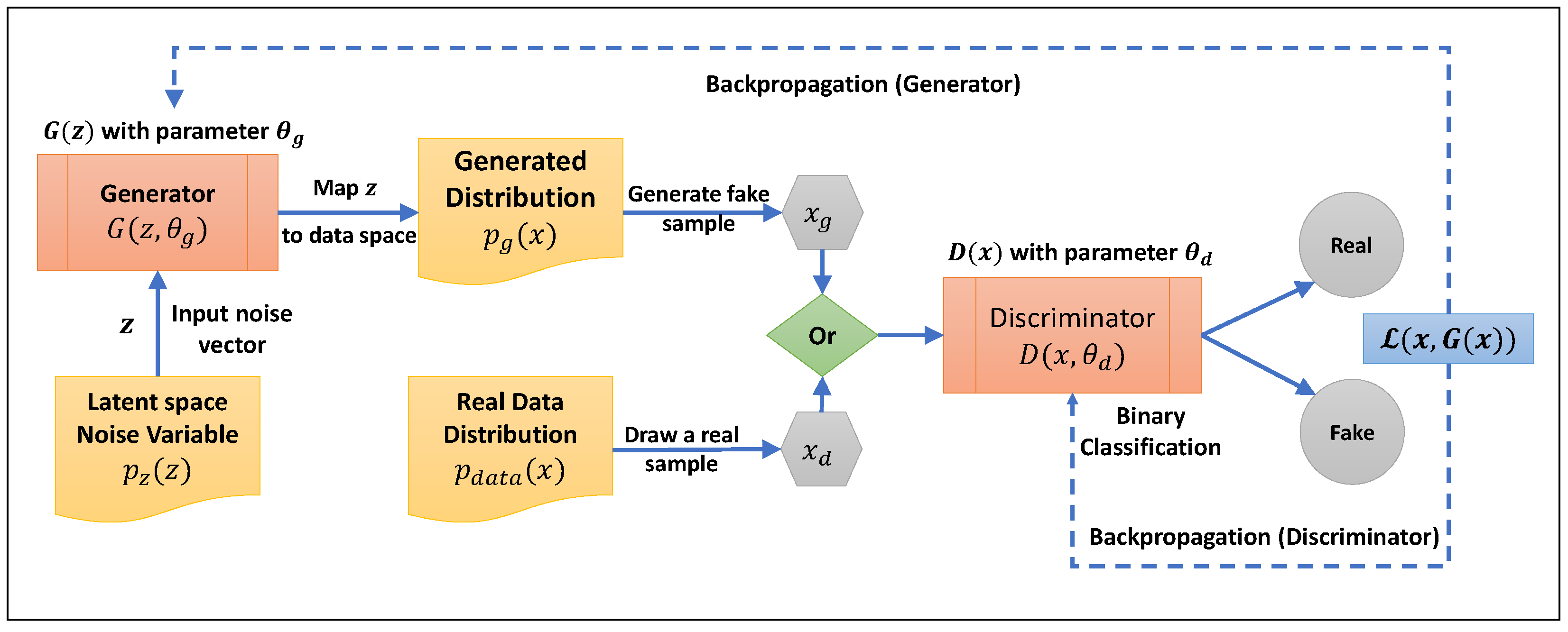
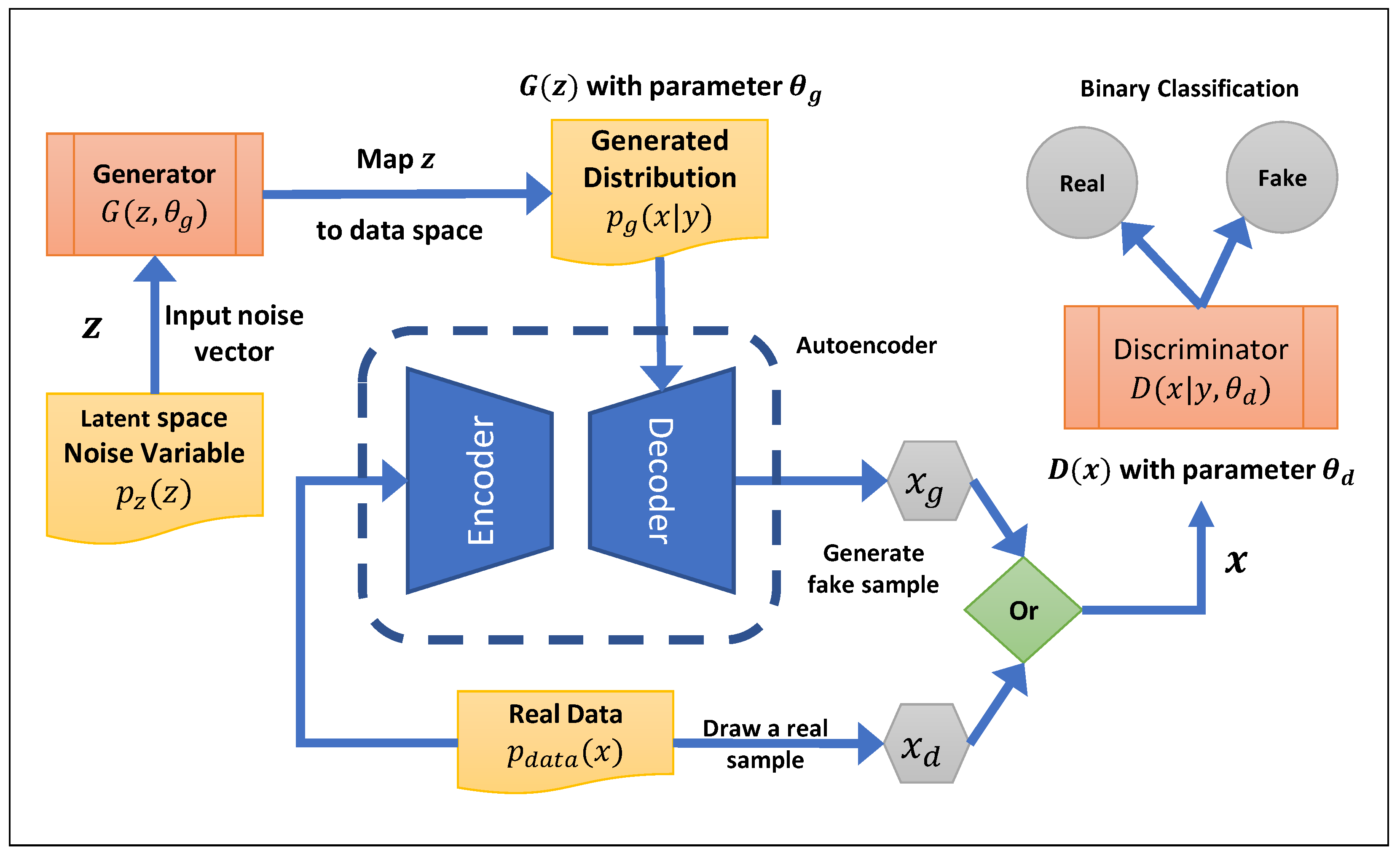
2.4. GAN-Based Tabular Generator

GANs were introduced in computer vision, where they are commonly used to process image data via Convolutional Neural Networks (CNNs). However, they are capable of generating tabular data as well. The GAN architecture has undergone numerous enhancements in recent years as a result of improvement to the architecture among the research community over the past few years [26]. To determine whether or not GAN is an appropriate option for synopsis generation, first we provide a detailed description of the GAN method and its architecture.
Generative Adversarial Networks are characterized by two neural networks: the generator, which creates data that are intended to mimic the true data distribution, and the discriminator, which evaluates the data to distinguish between the generator’s fake data and the real data from the actual distribution [27]. The generator draws a random vector z from the latent space with the distribution p z ( z ) . The generator G ( z ; θ g ) then uses a parameter θ g to map z from the latent space to the data space. Therefore, p g ( x ) (the probability density function over the generated data) is used by G ( z ) to generate x g . Then, the discriminator neural network D ( x ; θ d ) receives randomly either x g (the generated sample) or x d a t a (the actual sample) from the probability density function over the data space p d a t a ( x ) . The discriminator neural network D ( x ; θ d ) is a binary classification model in which D ( x ) returns the probability that x is derived from real data. Therefore, the output of this function is a single scalar that indicates if the passed sample is real or fake. Figure 2 depicts the described process and GAN architecture. The variables θ g and θ d are the weights of the generator and discriminator that are learned through the optimization procedure during training.
The goal of the discriminator in training is to maximize the probability that a given training example or generated sample is assigned the proper label, whereas the goal of the generator is to minimize the probability that the discriminator detects real data. Therefore, the objective function can be expressed as a minimax value function, V ( G , D ) , which is jointly dependent on the generator and the discriminator, where:
min G max D V ( D , G ) = E x p d a t a ( x ) [ log ( D ( x ) ) ] + E z p z ( z ) [ log ( 1 D ( G ( z ) ) ) ] .
The discriminator performs binary classification, which gives a value of 1 to real samples ( x p d a t a ( x ) ) and a value of 0 to generated samples ( z p z ( z ) ). Therefore, in the optimal adversarial networks, p g converges to p d a t a and the algorithm is stopped at D ( x ) = 1 / 2 , which means the global optimum occurs when p g = p d a t a [27].
The generation of data in an unconditioned GAN is completely unmanageable in a multimodal distribution. Mirza and Osindero [28] introduced a conditional version of GAN that can provide generators with prior information so that they can control the generation process for different modes. Achieving this objective requires conditioning the generator and discriminator on some additional information, y, where y can be anything from class labels to information about the distribution of data (modes). This can be done by giving the discriminator and the generator Y as an extra input layer in the form of a one-hot vector. In fact, the input noise p z ( z ) to the generator is not truly random if the information y is added to it, and the discriminator does not only regulate the similarity between real and generated data but also the correlation between the generated data and input information y. Therefore, the objective function in Equation (1) can be rewritten as follows:
min G max D V ( D , G ) = E x p d a t a ( x ) [ log ( D ( x | y ) ) ] + E z p z ( z ) [ log ( 1 D ( G ( z | y ) ) ) ] .
Figure 3 illustrates the structure of a CGAN and how the input information is applied during the process. A majority of applications for conditional GAN are concerned with synthesizing images by giving the label for the image that should be generated. Nonetheless, in the case of tabular data, this could be the shape of data on a multimodal distribution and can be used to inject information as prior knowledge to the generator.
To date, all proposed solutions have been published with the aim of adhering to real data privacy regulations and preventing data leakage during data sharing or for the generation of synthetic data for data imputation and augmentation. By contrast, in AQP applications, it is necessary to generate realistic data rather than synthetic data that is as close to real data as possible. The challenges associated with generating tabular data using GAN have been addressed in a few publications since 2017. The purpose of this section is to introduce promising variants of GAN for tabular data generation, followed by a classification of the proposed solutions based on the previously discussed synopsis construction challenges.
Choi et al. [29] proposed the medical Generative Adversarial Network (medGAN) to generate realistic synthetic patient records based on real data as inputs to protect patient confidentiality to a significant extent. The medGAN generates high-dimensional, multi-label discrete variables by combining an autoencoder with a feedforward network, batch normalization and shortcut connections. With an autoencoder, flow gradients are able to end-to-end fine-tune the system from the discriminator to the decoder for discrete patient records. The medGAN architecture uses MSE loss for numerical columns, cross-entropy loss for binary columns, and the ReLU activation function for both the encoder and decoder networks. The medGAN uses a pre-trained autoencoder to generate distributed representations of patient records rather than directly generating patient records. In addition, it provides a simple and efficient method to deal with mode collapse when generating discrete outputs using minibatch averaging.
Figure 4 shows the medGAN architecture and defines the autoencoder’s role in the training process.
The generator cannot generate discrete data because it must be differentiable. To address this issue, Mottini et al. [30] proposed a method for generating realistic synthetic Passenger Name Records (PNRs) using Cramer GAN, categorical feature embedding, and a Cross-Net architecture for the handling of this issue (categorical or numerical null values). As opposed to simply embedding the most probable category, they used the weighted average of the embedded representation of each discrete category. The embedding layer is shared by the generator and discriminator, resulting in a fully differentiable process as a result of this continuous relaxation. For handling null values, they are substituted with a new category in categorical columns. However, continuous columns fill null values with a random value from the same column and then a new binary column is inserted with 1 for filled rows and 0 otherwise. These additional binary columns are encoded like category columns. It should be noted that in this architecture, both the generator and discriminator consist of fully connected layers and cross-layers. Also, except for the last layer (sigmoid), all layers of the generator use leaky ReLU activations for numerical features and softmax for categorical features. However, the discriminator uses leaky ReLU activations in all but the last layer (linear). Neither batch normalization nor dropout are used in this architecture as in the Wasserstein and Cramer GAN [31]. Data pre-possessing in this algorithm is depicted in Figure 5.
As indicated, discrete values will be embedded using the embedding matrix; then, they will be concatenated with continuous columns of input data.
Table-GAN [32] uses GAN to create fake tables that are statistically similar to the original tables but are resistant to re-identification attacks and can be shared without exposing private information. Table-GAN supports both discrete and continuous columns and is based on Deep Convolutional GAN (DCGAN) [33]. Besides the generator and discriminator with multilayer convolutional and deconvolutional layers, the table-GAN architecture also includes a classifier neural network with the same architecture as the discriminator. However, it is trained using ground-truth labels from the original table to increase the semantic integrity of the generated records. Information loss and classification loss are two additional types of loss introduced during the backpropagation process. These functions serve a critical role in balancing privacy and usability while also ensuring the semantic integrity of real and generated data. Information loss functions by comparing the mean and standard deviation of real and generated data. This comparison aims to measure the discrepancy between them. It determines whether they possess statistically similar features from the perspective of the discriminator. On the other hand, classification loss measures the disparity in labeling. It assesses the difference between the actual label of a record and how the classifier predicts it should be labeled. Figure 6 is a representation of the loss functions in the table-GAN architecture.
Xu and Veeramachaneni developed TGAN [34], which is a synthetic tabular data generator for data augmentation that can take into account mixed data types (continuous and categorical). TGAN generates tabular data column-by-column using a Long Short-Term Memory (LSTM) network with attention. The LSTM generates each continuous column from the input noise in two steps. First, it generates a probability that the column comes from mode m, and then, it normalizes the column value based on this probability. TGAN penalizes the original loss function of a GAN by incorporating two Kullback–Leibler (KL) divergence terms. These terms measure the divergence between generated and real data for continuous and categorical columns separately [35]. Therefore, the generator is optimized as follow:
L G = E z N ( 0 , 1 ) [ log ( D ( G ( z ) ) ) ] + i = 1 N c K L ( u i , u i ) + i = 1 N d K L ( d i , d i ) .
where u i and u i are probability distributions over continuous column c i for generated and real data, respectively, d i and d i are the probability distributions over categorical column d i using the softmax function for generated and real data, respectively, N c is the number of continuous columns, and N d is the number of categorical columns. The authors also proposed a conditional version of TGAN, named CTGAN [36], for addressing data imbalances and multimodal distribution problems by designing a conditional generator with training by a sampling strategy to validate the generator output by estimating the distance between the conditional distributions over generated and real data.
CTAB-GAN [37] was introduced with the ability to encode a mixed data type and a skewed distribution of the input data table; it utilizes a conditional generator, information and classification loss functions derived from table-GAN, as well as CNNs for both the generator and discriminator functions. Since CNNs are effective at capturing the relationships between pixels within an image, therefore, they can be employed to enhance the semantic integrity of created data. However, in order to prepare data tables for feeding the CNN, rows are transformed into the nearest square d × d matrix, where d = C e i l ( N c + N d ) , N c and N d are the number of continuous and categorical columns, respectively, in a row of the data table, and then, the extra cells values ( d × d ( N c + N d ) ) are padded with zeros.
It is difficult for GAN to control the generation process of data-driven systems; therefore, integrating prior knowledge about data relationships and constraints can assist the generator in generating synopses that are realistic and meaningful. In order to implement this, DATGAN [38] incorporates expert knowledge into the GAN generator by matching the generator structure to the underlying data structure using a Directed Acyclic Graph (DAG). Using DAG, the nodes represent the columns of a data table, while the directed links between them allow the generator to determine the relationship between variables so that one column’s generation influences another. This means if two variables have no common ancestors, they will not be correlated in the generated dataset. In relational databases, there is no particular order in which columns appear in data tables. Nevertheless, the DAG enables data tables to have a specific column order based on their semantic relationship.

2.5. Tabular GAN Evolution

GAN has made significant progress in recent years, which has led to the development of novel variants that improve previously introduced versions that had promising results prior to their introduction. Table 1 provides a summary of the variants of GAN that have been discussed in this paper and highlights the specific architectural advancements and loss functions that have been employed to enhance the performance of each variant. MedGAN, for example, aims to generate high-dimensional discrete columns while avoiding the common pitfall of mode collapse by leveraging an autoencoder network alongside a Feedforward Neural Network (FNN) for generation and a Fully Convolutional Network (FCN) for discrimination. PNR-GAN addresses the challenge of null values in data tables by employing a cross-layer FCN for both the generator and discriminator and utilizes Cramer loss to measure discrepancies. Table-GAN and CTAB-GAN employ Convolutional Neural Networks (CNNs) in their generators to capture the spatial hierarchy of features within tabular data, with CTAB-GAN incorporating conditions from CGAN and AC-GAN for more-targeted data synthesis. CTGAN also adopts this conditional approach but further refines the model to handle non-Gaussian and multimodal distributions effectively by utilizing Wasserstein loss with a gradient penalty for a more stable training process. On the other hand, TGAN and DATGAN leverage Long Short-Term Memory (LSTM) networks in their generators to capture temporal dependencies and correlations within data: a crucial aspect for maintaining integrity when generating sequential or time-series data. These models demonstrate the ongoing refinement of GANs for complex data structures, where the goal is not only to generate new data but to do so with an acute awareness of the inherent relationships within the original dataset.
Figure 7 provides a visual representation of the progression and diversification of GAN architectures as they have been specialized for tabular data generation. The diagram traces the lineage of various GAN models starting with the inception of the original GAN framework in 2014. It distinguishes between architectures developed for non-tabular data (in green) and those specifically tailored for tabular data (in yellow), underscoring how foundational models have been adapted and extended to meet the unique challenges of tabular datasets. The evolutionary trajectory begins with the general-purpose GAN and branches into models like DCGAN, which introduced convolutional layers for improved performance on image data. From there, tabular-specific adaptations emerge and innovations continue with the integration of LSTM in TGAN and DATGAN to capture the sequential relationships within data and conditional mechanisms in CTGAN and CTAB-GAN for generating data with given constraints. The figure encapsulates the dynamic and branching nature of GAN development and highlights the critical adaptations made to leverage the power of GANs in the realm of structured data synthesis.

3. Synopsis Construction Challenges

Traditional methods for synopsis construction have many challenges related to data type, structure, distribution, and query aggregation functions. Furthermore, synopses provide the most accurate summary using the entire data stream, and it is inconvenient to retrieve the entire dataset in real-time databases as it changes over time. According to the data structure of relational databases, the challenges associated with generating synopses can be categorized into many significant groups [34].

3.1. Data Type

It is challenging to construct a data synopsis that is representative of the entire data table due to the difference in data types. For instance, different activation functions on the output are required for generative models since relational database tables include numerical, categorical, ordinal, and mixed data types. As an example of a mixed data type, a financial database contains columns for loan debts, wherein a loan holder may have no debt or debt with a positive value [37]. In data analysis, this can be defined as categorical data using a step function, but in reality, it is continuous data. In this regard, a data generator must be able to detect these types of data in order to avoid adverse effects on the interpretation of the data. The several types of data used to create AQP data synopses are broken down in Table 2. We mention that textual data types are not typically utilized in AQP queries and are therefore ignored here.

3.2. Bounded Continuous Columns

Continuous column C i is bounded if there are two numbers a and b for which for all x X   a x b . The intricacy of synopsis construction for these bounded continuous columns arises from the necessity to sample from a probability distribution that not only mirrors the true underlying statistical characteristics of the original data but also adheres strictly to these boundary constraints. For instance, a credit card’s expenditure column might be restricted from zero to an upper limit reflecting the credit limit; hence, the synthetic data generation process must respect these limits to produce meaningful and applicable synthetic transactions. The challenge intensifies as it requires the synthesis process to be sensitive to the distribution’s tails and to avoid the generation of outliers that fall outside the established bounds, which would otherwise lead to unrealistic and operationally irrelevant data points.

3.3. Non-Gaussian Distribution

When dealing with the non-Gaussian distributions that are common in real-world datasets, the assumption of normality often fails in the field of synopsis construction. Such distributions may be multimodal: containing several peaks or modes that reflect the complexity of underlying data-generation processes. For instance, the distribution of incomes in a socio–economic dataset could exhibit multiple modes corresponding to different socio–economic classes. Traditional synopsis generation techniques may inadequately capture the multimodal structure of such distributions, leading to the absence of entire modes. This results in a generated synopsis that fails to represent segments of the population within the original dataset [34].
Moreover, the presence of long-tailed distributions poses additional challenges [37]. These distributions are characterized by a proliferation of infrequent events, such as a customer purchase history for which the vast majority of customers make infrequent purchases while a minor fraction exhibits high purchase frequencies. Synthesizing data from such a distribution requires not only capturing the frequent low-occurrence events but also accurately representing the rare high-occurrence instances. Conventional methods may struggle with this: often either over-representing the tail and creating too many rare events or under-representing it and thus failing to capture the true nature of the underlying data. This misrepresentation can skew the synopsis, rendering it less effective for use in decision-making processes for which an understanding of rare events is critical.

3.4. Imbalanced Categorical Columns

In the construction of data synopses, the handling of imbalanced categorical columns presents a significant challenge [34]. Categorical variables in real-world datasets frequently show a skewed distribution in terms of the frequency of occurrence across categories. The presence of such a disparity indicates that minority categories make only a small contribution to the overall distribution of data, which may result in their under-representation in the generated synopsis. The process of creating synopses is influenced by a lack of representation of certain classes and results in bias towards the majority class due to its higher statistical likelihood. For instance, consider a customer gender column in a retail database with a pronounced imbalance where ‘male’ customers vastly outnumber ‘female’ customers. A synopsis generated from this distribution might reflect this skew, resulting in a synthetic dataset dominated by ‘male’ entries. However, this skew inaccurately portrays the significance of the ‘female’ category, which, despite its smaller size, may carry substantial weight in consumer behavior analysis.

3.5. Semantic Relationships and Constraints

Tabular data often includes complex semantic relationships that are not easily understood through standard statistical analysis [39]. These relationships can exist between categorical and numerical columns alike and are crucial for maintaining the integrity and usefulness of the generated synopsis. Identifying and encoding such relationships is a challenge due to the heterogeneity of domain-specific constraints and the complex nature of the inter-column dependencies, which may not be amenable to simple rule-based generalizations. For instance, semantic relationships may determine that certain numerical values possess validity solely when paired with specific categorical entries, imposing a constraint-based association. Alternatively, a rule-based linkage could suggest a probabilistic co-occurrence pattern between different fields in the data. Hence, it is imperative for a comprehensive process of generating synopses to include mechanisms that can deduce these complex relationships, which can be multi-faceted and deeply embedded within the structure of the data. A failure to do so not only compromises the authenticity of the synthesized data but also limits the operational relevance of the synopsis, as it could lead to the generation of implausible or inconsistent records that do not adhere to the real-world rules and constraints governing the dataset. Figure 8 represents two examples of generated samples from a table that the model should reject semantically. To generate a representative data synopsis in AQP, the city must be properly associated with the state, and the joined column cannot precede the founded column.

4. GAN-Based Synopsis Construction Solutions

It is possible to categorize synopsis construction solutions into three different categories: Data Transformation, which addresses data type issues; Distribution Matching, which addresses ranges and distributions of data; and Conditional and Informed Generation, which addresses imbalance classes, semantic relationships, and table constraints.

4.1. Data Transformation

Mode normalization is capable of detecting modes of data by assigning samples to different modes and then normalizing each sample based on the corresponding mode estimator [40]. To deal with multimodal distributions for continuous columns, mode-specific normalization is introduced in TGAN [34]. Using this algorithm, first, the number of continuous columns’ modes is calculated using Gaussian kernel density estimation. Then, the Gaussian Mixture Model (GMM) can be employed to efficiently sample values from a distribution with multiple modes by clustering the values of continuous columns ( C i ). In other words, the weighted sum of the Gaussian distributions over C i can represent the multimodal distribution over it. A normalized probability distribution over m Gaussian distributions can then be used to represent each continuous column so that each column can be clustered into m fixed Gaussian distributions. As a result, if there are fewer than m modes in one column, then the probability of that mode is high, and for the rest, it is close to zero. However, in CTGAN [36], first, a Variational Gaussian Mixture (VGM) model should be applied to each continuous column ( C i ) in order to fit a Gaussian mixture and find the number of modes (m). Then, a one-hot vector ( β i , j ) indicates to which mode a given value belongs, and a scalar ( α i , j ) serves as the value itself within that mode. For the learned Gaussian mixture for column C i with m modes, the following equation is given:
P C i ( c i j ) = k = 1 m w k N ( c i j ; μ k , σ k ) .
where c i , j is value of the j t h row from the i t h column, μ k and σ k are the mean and standard deviation, respectively, of the Gaussian distribution for the k t h mode, and w k is the weight of the k t h mode. For each value, the probability density ρ of k t h mode is:
ρ k = w k N ( c i j ; μ k , σ k ) .
Therefore, each value can be normalized according to the mode with the highest probability. As an example, the values of α and β related to column c i , j in the k t h mode will be:
α i , j = c i , j μ k λ σ k , β = [ 0 , 0 , ,   1   k t h element , , 0 , 0 ] .
where λ is a parameter specified by the modeler.
For categorical columns D, the situation is different; TGAN [34] is stated to convert these columns ( d i j ) to a representation using one-hot encoding with added noise ( U n i f o r m ( 0 , γ ) , where γ is an arbitrary number). To achieve this, after creating the one-hot vector, noise will be added to each element, and the resulting representation will be renormalized. Therefore, each data row can be represented by a concatenation of continuous and categorical columns as follows:
r o w j = α 1 , j β 1 , j . . . α N c , j β N c , j d 1 , j . . . d N d , j .
where d i , j is the one-hot representation of a categorical column, N c is the number of continuous columns, and N d is the number of categorical columns D i . The direct sum operator ⊕ combines the contributions of different vectors or matrices to form a new vector r o w j . Each component represents a different subspace or block in the final vector.
As previously discussed, columns can be considered mixed if they contain both categorical and continuous values or continuous values with null values. The encoding process for continuous and categorical columns in CTAB-GAN [37] is exactly the same as CTGAN [36] by defining α and β . However, in mixed-type columns, the encoder is defined so that each column is considered a concatenation of value–mode pairs, where the categorical part of values takes zero for α and is treated as continuous. Figure 9 shows the distribution over an arbitrary mixed-type column with two modes for continuous ( m 2 , m 3 ) and two categorical parts ( m 1 , m 4 ) and illustrates how this algorithm transforms one row of mixed-mode data.

4.2. Distribution Matching

In order to generate synopses with the same distribution as the underlying distribution, the training algorithm should penalize the generator. Information loss [32] helps the generator generate synopses statistically closer to the real ones. It utilizes the statistical characteristics L m e a n (first-order statistics, Equation (8)) and L s d (second-order statistics Equation (9)) of the extracted features prior to the classifier in the discriminator to penalize the generator for the discrepancy between real and generated data. This makes sense because the extracted features are used to determine the binary decision of the discriminator.
L m e a n = E [ f x ] x p d a t a ( x ) E [ f G ( z ) ] z p z ( z ) 2 .
L s d = SD [ f x ] x p d a t a ( x ) SD [ f G ( z ) ] z p z ( z ) 2 .
where f represents features, E [ f ] is the average, and SD [ f ] is the standard deviation of features over all rows in the data table. The Euclidean norm is used to measure the discrepancy between two terms. As we discussed before, table-GAN [32] was developed to protect confidential data privacy when they are shared with the public. As a result, it should be possible to control the similarity of generated data with real data during the generating process. To this end, information loss for the generator is demonstrated as follows:
L i n f o G = max ( 0 , L m e a n δ m e a n ) + max ( 0 , L s d δ s d ) .
where δ is a threshold indicating the quality degradation of generated data, and max ( . ) represents the hinge-loss, which is zero until δ is reached. However, in AQP, it is not necessary to meet this threshold in order to generate realistic data synopses.
DATGAN [38] uses the improved version of the Wasserstein loss function in WGAN [41] in addition to the Vanilla GAN loss function with a gradient penalty [42] and also adds the KL-divergence as an extra term to the original loss function. Both of these terms aim to minimize the difference between the probability distributions of real and generated data. WGAN employs an alternative method to train the generator to better approximate real data distributions. This approach replaces the discriminator model with a critic that scores the degree to which a data sample is real or fake rather than using the discriminator as a classifier. Therefore, WGAN considers the discriminator output as a scalar score instead of a probability, and Wasserstein loss ensures a greater difference between the scores for real and generated data. As a result, the network can prevent vanishing gradients in the generator models. However, the WGAN’s primary problem is that it must clip the weights of the critic in order to enforce the Lipschitz constraint. This issue can be addressed by adding a gradient penalty to the critic. Equation (11) shows the Wasserstein objective function, and Equation (12) shows the same with a penalty on the gradient norm for random samples x ^ p x ^ .
min G max D V ( D , G ) = E x p d a t a ( x ) [ D ( x ) ] E z p z ( z ) [ D ( G ( z ) ) ] .
L W = E z p z ( z ) [ D ( G ( z ) ) ] E x p d a t a ( x ) [ D ( x ) ] + λ E x ^ p x ^ [ | | x ^ D ( x ^ ) | | 2 1 ) 2 ] .
where λ is a parameter defined by the modeler and x ^ sampled from G ( z ) and x.

4.3. Conditional and Informed Generator

Imbalances in categorical columns can cause inaccuracies when generating synopses and may result in the generator not being trained to match the distribution of the real data. In CTGAN [36], the conditional generator is introduced (using training-by-sampling) as a solution to this problem. To this aim, the generated value can be interpreted as a conditional distribution of rows given the value of an imbalanced categorical column. Therefore, the original distribution can be reconstructed as follows:
P g ( r o w | D i = k ) = P ( r o w | D i = k ) = > P ( r o w ) = k D i P g ( r o w | D i = k ) P ( D i = k ) .
where k is a value in the i t h categorical column D i . For the implementation of this solution, a conditional vector consisting of a mask vector that represents the address of the table value (column and corresponding row value) is required. This conditional vector does not guarantee the feedforward pass obtains the correct value based on the mask vector M; instead, the suggested approach penalizes the conditional generator’s loss by averaging the cross-entropy between the generated M ^ i and the expected conditional vector M i over all instances of the batch. The generator loss can be expressed as follows:
L G = E [ H ( M i , M ^ i ) ] .
where H ( . ) is the cross-entropy between two values. As a result, the generator learns to replicate the masked value in the generated row during training. The conditional vector for a data table with N categorical columns is the direct sum of all mask vectors (M) across each column D i , where for each value c i , j :
M i = 1 if j t h value 0 the rest , c o n d = M 1 M N .
In fact, generator loss allows the generator to learn to produce the same classes as the given conditions. Mask vectors ( M i ) are initialized with 0 for each categorical column ( D i ) during the conditional generator procedure. Then, a column is chosen at random, and the Probability Mass Function (PMF) is applied to the column’s range of categories. According to PMF, one category is then picked, and its value in the corresponding mask vector is changed to 1. Finally, the conditional vector is formed, and the generator is able to generate a synthetic row for the given categorical column. Figure 10 represents a mask vector generation process for a data table with N d categorical columns when the generator is conditioned for the j t h category of the i t h categorical column.
It has been discussed previously that columns in a table may have a meaningful relationship with one another. CTAB-GAN [37] utilizes a classifier neural network using Auxiliary Classifier GAN (AC-GAN) [43], which is a conditional GAN type that requires the discriminator to predict the class label c p c of generated data as well as the realness classifier. In AC-GAN, the generator generates a new sample using noise z and a class label c, while the discriminator provides both a probability distribution over sources P ( S | X ) and a probability distribution over class labels P ( C | X ) . The objective function contains the following terms:
L S = E x p d a t a ( x ) [ log P ( S = r e a l ) ] + E x p z ( z ) [ log P ( S = f a k e ) ] .
L C = E x p d a t a ( x ) [ log P ( C = c r e a l ) ] + E x p z ( z ) [ log P ( C = c f a k e ) ] .
where L S is the likelihood of predicting the correct source, L C is the likelihood of predicting the correct class, and c is a class label. The discriminator is trained to maximize L C + L S , and the generator is trained to maximize L C L S . These objective functions allow the training procedure to generate data according to a specific type of data, while the discriminator must predict the class label of the generated data and determine whether or not it is real. As a result of this, the classifier loss (Equation (18)) is added to the generator in CTAB-GAN to increase the semantic integrity of generated records and to penalize the generator when the combination of columns in a data row is semantically incorrect.
L c l a s s G = E z p z ( z ) [ | l ( G ( z ) ) C ( f e ( G ( z ) ) ) | ] .
where l ( . ) returns the target label and f e ( . ) returns the input features of a given row.
As mentioned before, DATGAN [38] uses DAG to control the generation process based on semantic relationships and correlations between columns. According to the constructed DAG, each column and its sequence are represented by Long Short-Term Memory (LSTM) cells. Therefore, by providing the generator with prior knowledge, DAG decreases the GAN’s capacity to overfit noise in the training process and enables the GAN to produce more accurate data by using this noise more efficiently. Inputs and outputs of LSTM cells should be modified in accordance with the GAN architecture. Inputs can be expressed as follows:
i t = a t f t 1 z t .
where z t is a tensor of Gaussian noise, which is the concatenation of the noise from the source nodes at each node of the DAG. The variable f t 1 is the transformed output of the previous tensor ( h t 1 ). For the purposes of determining which previous cell outputs are relevant to a node input, a t represents a weighted average of all ancestor LSTM outputs. Therefore, a t and z t are defined based on all ancestors of the current node. Data input into DATGAN architecture (generated and real data) should be encoded into [−1,1] or [0,1] using the techniques described in Section 4.1. Additionally, for categorical columns, generators produce a probability over each class, making it easy for a discriminator to differentiate between real and created values. Therefore, DATGAN recommends using one-sided label smoothing for the default loss. This means categorical 0,1 vectors are introduced with additive uniform noise and then rescaled to [0,1] bound vectors. Figure 11 illustrates the DATGAN process flow diagram, including the data transformer and label smoothing.
In this algorithm, DAG is generated manually; therefore, semantic relationships between variables should be injected as expert knowledge and cannot be detected by the model. However, tabular data cannot be considered sequential since the order of columns in a data table is generally random. Therefore, a DAG is used to create a specific sequence of columns.
The solutions presented in this section directly counter the challenges identified in Section 3, thereby underscoring the robustness and versatility of GAN-based synopsis construction. Specifically, ‘Data Transformation’ effectively addresses issues related to data types and structures and ensures that synopses are both accurate and representative of the underlying database despite its evolving nature. ‘Distribution Matching’ adeptly handles the complexities of data ranges and distributions: a critical aspect for maintaining the integrity and utility of the synopsis. Lastly, the ‘Conditional and Informed Generator’ approach is instrumental for overcoming challenges related to imbalanced classes, semantic relationships, and table constraints, thereby enhancing the synopsis’s relevancy and applicability in real-time database environments. This comprehensive alignment of challenges and solutions highlights the innovation and practicality of our GAN-based approach for synopsis construction for Approximate Query Processing and marks a significant advancement in the field.
While the application of a Generative Adversarial Network (GAN) in synopsis construction for Approximate Query Processing (AQP) marks a significant stride forward, it is important to acknowledge certain inherent limitations. Firstly, the effectiveness of GAN is heavily contingent on the volume and quality of training data. In scenarios where data are sparse or of poor quality, GAN may struggle to generate accurate and representative synopses [44]. Secondly, the complexity of GAN architectures and the need for extensive hyperparameter tuning can pose challenges, particularly in terms of computational resources and time required for model training and optimization [45]. Another limitation lies in the GAN’s ability to capture and maintain complex semantic relationships and constraints within the data: a critical aspect in relational databases [38]. This often necessitates additional layers of complexity in the model architecture, further escalating the computational demands [44]. Lastly, despite advancements, there remains a degree of unpredictability and lack of interpretability in the outputs generated by GAN, which can be a significant drawback in decision-making contexts where transparency and explainability are paramount. Acknowledging these limitations is crucial for setting realistic expectations and guiding future research towards addressing these challenges and thereby enhancing the practical applicability of GAN-based AQP in data-driven systems.

4.4. Comparative Analysis of GAN-Based Methods

Table 3 presents a comparative analysis between GAN-based methods and traditional methods for synthetic data generation. It highlights GAN’s superiority in handling complex, high-dimensional data and producing highly realistic outputs [46]. The table also emphasizes the versatility and adaptability of GAN-based methods in various domains, showcasing their innovation potential and advanced capabilities in data augmentation and privacy preservation [47]. Conversely, traditional methods are noted for their simplicity and direct control over data, but they fall short in terms of complexity, realism, and adaptability.

5. Synopsis Evaluation and Error Estimation

To avoid performing expensive computations and to take a trial-and-error approach, AQP requires an estimation of errors before running the query. As a result, the AQP system is able to select the optimum synopsis type and resolution based on the user’s latency or accuracy requirements. Error Quantification Modules (EQMs) in AQP systems perform this process by measuring the quality of responses either by predicting or by running queries on synopses [18]. A broad classification of the criteria for evaluating approximate query processing systems can be made as follows [48]:
  • Query Type: In terms of aggregation functions and conditions, what types of queries are covered by the methods?
  • Time Complexity: How long does it take to produce the synopses and return an approximate result?
  • Space Complexity: What is the required storage space for data synopses?
  • Accuracy: Does the approximate answer meet the error confidence interval?
In this study, however, the focus is on the creation and quality of synopses; therefore, this section discusses the synopsis evaluation technique rather than the EQM process. Different aggregation functions necessitate unique considerations when creating a synopsis. For example, min() and max() require that the synopsis include the critical outliers, which contain critical information. For instance, as depicted in Figure 12, a single transaction in a real-world database may contain vital information and influence decisions based on business problems. As can be seen in this figure, a food supplier sells its product to both retailers and wholesalers. Although retailers make the majority of sales transactions, wholesalers can place orders that are more significant in terms of quantity and cost.
Likewise, count() and sum() may return unacceptable results for minority groups if the query aggregates groups by those columns. Avg() can also be sensitive in situations where a query filters data based on specific conditions or criteria.
In generative models, evaluation methods cannot be generalized to other contexts; instead, they must be evaluated explicitly based on their application. During the optimization of these models, Gaussian distributions are fitted to a mixture of Gaussian distributions by minimizing distance measures such as Maximum Mean Discrepancy (MMD) [49] and Jensen–Shannon divergence (JSD). Minimizing MMD or JSD results in the omission of some modes in a multimodal distribution. In addition, maximizing the average log-likelihood or minimizing the KL-divergence can assign large probabilities to non-data regions. In image synthesizing applications, three common criteria are used to evaluate generative models: log-likelihood, Parzen window estimates, and visual fidelity of samples [50]. However, the evaluation of results for tabular data with complex data types and distributions would be quite different.
In the pursuit of evaluating the fidelity of generated data synopses to their original datasets, it is imperative to establish that the synthetic data closely reflects the properties and structure of the real data it aims to mimic. The SDMetrics Python library [51] offers a comprehensive suite of metrics designed to assess both the quality and the privacy of synthetic datasets. For the scope of this study, the primary focus is on the quality aspect of the synthetic data as privacy concerns, while important, are beyond the study’s aims and could potentially compromise data utility. To contextualize the effectiveness of different data generation methodologies, this study employs the Adult dataset [52]—a commonly used benchmark in the field. The dataset comprises 15 attributes encompassing a mix of six numerical and nine categorical columns: thereby presenting a varied set of challenges in data generation.
The evaluative framework categorizes the analysis into four distinct dimensions: Data Coverage, Data Constraint, Data Similarity, and Data Relationship. These dimensions collectively capture the extent to which the generated data mirror the real data in terms of distribution, constraints, patterns, and inherent relationships.
The experimental validation involves a comparative analysis of several data synopsis generation approaches. The Gaussian Copula [53] data generator [51] serves as a statistical benchmark and leverages classical methods to model and generate synopses. By contrast, the Variational Autoencoder [11] (VAE)-based data generator represents an approach grounded in the domain of deep generative models. The study further includes the Copula GAN data generator [51], which amalgamates classical statistical modeling with the advanced capabilities of GAN-based deep learning and aims to blend the strengths of both domains. Lastly, the CTGAN [36] data generator, which relies purely on GAN-based methodologies, is put to the test to generate data synopses. By comparing these diverse methods, the experiment seeks to provide a comprehensive evaluation of their performance in creating accurate and reliable data synopses for Approximate Query Processing (AQP).

5.1. Data Coverage

For discrete columns D i , we must determine whether all categories in the real data are represented in the synopsis. To accomplish this goal, a score is calculated by dividing the number of unique categories in the synopsis by the number of unique categories in the corresponding column of the actual data as follows:
c o v e r a g e D i = N D g N D d a t a i .
where i is the column index, N D g is the number of unique categories in the generated synopsis, and N D d a t a is the number of unique categories in the real data. When a column is scored 1, all of the unique categories in the actual data are present in the generated synopsis, while a score of 0 indicates that no unique categories are present in the generated synopsis. In the case of continuous columns, the coverage metric is used to measure whether a generated column in the synopsis covers the whole range of values that can be found in the real column. The coverage score for continuous columns is calculated as follows:
c o v e r a g e C i = 1 m a x m i n ( C g ) m i n ( C d a t a ) m a x ( C d a t a ) m i n ( C d a t a ) , 0 + m a x m a x ( C d a t a ) m a x ( C g ) m a x ( C d a t a ) m i n ( C d a t a ) , 0 .
where C g is the generated value and C d a t a is the real value of column C i . The goal of this metric is to determine how closely the min and max of the generated values match the actual min and max values. It is possible for Equation (21) to become negative if the range covered by the generated synopsis is inadequate, and in such a situation, it returns a score of 0 since this is the lowest possible result.
Figure 13 serves as an illustrative comparison of the real and generated distributions of the ‘age’ column from the Adult dataset generated by two different synthesis techniques: the (a) CTGAN-based approach and the (b) Variational Autoencoder (VAE). The coverage metric, as defined, assesses the span of generated data against the actual data’s range.

5.2. Data Constraint

In order to measure how a continuous column adheres to a boundary of real data, boundary adherence is introduced. The frequency of generated values within the minimum and maximum ranges of the real column values is calculated using this metric.
a d h e r e n c e C i = N ( m i n < x i < m a x ) N i .
where N i is the number of records in column C i . A column with a score of 1 indicates all values adhere to the boundaries of real data, while a column with a score of 0 indicates that no values fall between the minimum and maximum of the real data.
Figure 14 elucidates the boundary adherence of generated data for the ‘education-num’ column, which is an integer value intrinsically tied to education levels generated by VAE model. The metric presented assesses the generated data’s fidelity to the real data’s range, where adherence to the minimum and maximum boundary values is critical, as values outside this range would be nonsensical given the nature of the data.

5.3. Data Similarity

The Synthetic Data Metrics (SDMetrics) library [51] introduces several metrics for measuring data similarity. In order to calculate the similarity between real and generated marginal distributions, two types of metrics are available: the Kolmogorov–Smirnov (KS) statistic for continuous columns and the Total Variation Distance (TVD) for discrete columns. Based on the KS statistic, we can determine how much the empirical distribution function of the generated data differs from the Cumulative Distribution Function (CDF) of the real data. This means that in this case, the KS statistic represents the maximum difference between the two generated and real CDFs, as illustrated in Figure 15.
The KS statistic can be calculated using the following expression:
K S d a t a , g = s u p x F 1 , d a t a ( x ) F 2 , g ( x ) .
where F 1 , d a t a and F 2 , g are the empirical distribution functions of the real and generated data, respectively, and s u p is the supremum function.
In order to calculate the TVD statistic, we first computes the frequency of each category value in the real and generated columns and express them as probabilities. Once the frequencies are calculated, the TVD statistic compares the difference in probabilities using the following formula:
T V D d a t a , g = 1 δ ( X , G ) = 1 1 2 x D d a t a | X x , g G x , g | .
where x and g refer to all possible categories in discrete column D, and X and G represent the frequencies for those categories for real and generated data, respectively. The similarity score is considered the complement of a T V D , so a higher score indicates a higher level of quality.
Table 4 presents a comparative analysis of these metrics across all columns of the Adult dataset, with produced data generated by four different methods: Copula, CTGAN, VAE, and Copula-GAN. The values are indicative of the closeness of the generated data’s distribution to that of the real data.
A missing value (null value) can occur in many different situations in a real-world database [54]. This is why the missing-value similarity score has been introduced for the purpose of detecting these missing values when generating a synopsis. In this metric, the number of missing values in the generated data is compared to the number of missing values in the real data for each column. The metric can be applied to any column with any type of data. As part of this process, the proportion of missing values in both the real and synthetic data is calculated, and the normalized version of this (Equation (25)) results in a similarity score between 0 and 1, with 1 representing the highest level of similarity.
m i s s i n g = 1 | X p G p | .
where p is the proportion of missing values, and X and G represent the distributions for real and generated data, respectively. In addition, it is possible to measure the statistical similarity between a column of real data and a column of generated data using mean, median, and standard deviation using the following formula:
s i m i l a r i t y = max 1 | f ( x ) f ( g ) | | max ( x ) m i n ( x ) | , 0 .
where an arithmetic mean, median, or standard deviation is defined as f, and it returns a score between 0 and 1, where a high value represents a high degree of similarity.

5.4. Data Relationship

For measuring the semantic relationship and correlation between columns within a single data table, the contingency can be applied to discrete columns using crosstabulation (also known as a contingency table). This score is a matrix representation of the multivariate frequency distribution of variables. First, two contingency tables should be created over the categories present in each column in order to compare a discrete column in the real data with the corresponding column in the generated data. Indeed, the created tables summarize the proportion of rows in real and generated data that have each combination of categories. After that, the total variation distance is used to calculate the difference between the contingency tables. In this case, the distance would be between 0 and 1, so subtracting 1 from the score would indicate a high degree of similarity. Below is a formula that summarizes the process.
c o n t i n g e n c y x , g = 1 1 2 x D d a t a g D g | X x , g G x , g | .
where x and g refer to all possible categories in discrete column D, and X and G represent the frequencies for those categories for real and generated data, respectively. A score of 1 indicates the best contingency between real and generated data, and a score of 0 indicates the worst contingency. Also, a correlation similarity test can be applied to continuous columns by measuring the correlation between two numerical columns and computing the similarity between the real and generated data using Pearson’s and Spearman’s rank coefficients. Initially, a correlation coefficient should be calculated between two continuous columns in the real data and their corresponding columns in the generated data. Then, after normalizing two correlation values, the following equation returns a similarity score.
c o r r e l a t i o n x , g = 1 | X x , g G x , g | 2 .
where x and g refer to all values in continuous column C, and X and G represent the distributions for real and generated data, respectively. In this score, the correlation between the columns is bounded between −1 and 1, with −1 representing the most negative correlation and 1 representing the most positive correlation between the real and generated columns.
Traditionally, relational databases are divided into separate tables for each object, and to retrieve information from those tables, related fields within the tables need to be linked together by defining relationships. Users can then retrieve information from multiple tables simultaneously by calling queries [55]. In terms of measuring the similarity among those tables, the cardinality of related tables can be used. The cardinality of a table relationship is determined by how many rows in each table are related. Therefore, when generating synopses, measuring whether a table’s cardinality is the same between the real and generated data is an important metric. In order to measure the similarity of cardinality between related tables, the marginal distribution can be utilized by computing the similarity between a real and generated cardinality distribution using the KS or TVD score. In the case of real and generated data, the cardinality complement score returns 1 when the cardinality values are the same and 0 when they are different.

6. Conclusions

The construction of synopses is essential for data-driven decision-making systems in order to provide approximate answers to queries. Since traditional statistical approaches are ineffective, many researchers are exploring how realistic data can be generated with Deep Generative Models in order to revolutionize the AQP system. In this paper, we discussed the challenges associated with the generation of synopses in relational databases and whether Generative Adversarial Networks can be used to accomplish this task. Furthermore, we summarized and reformed statistical metrics for evaluating the quality of the generated synopses as a part of this study.
There is no doubt that GAN has an incredible ability to generate realistic images and videos. However, each data point in an image is represented by a pixel, which cannot be interpreted alone but only in relation to the other pixels in the image. Consequently, the meaning of the same pixel in one image differs from the meaning of the corresponding pixel in another image [38]. In contrast to images, data tables typically contain columns that have a specific meaning and can be understood by their positions and values, and their values may also have semantic relationships with each other. We analyzed the challenges associated with synopsis construction in a relational database and categorized them into the following categories: data type, bounded continuous columns, non-Gaussian distribution, imbalanced categorical columns, and semantic relationship and constraint between columns. Then, by reviewing the promising variants of GAN designed for generating tabular data, we realized that the solutions to the given challenges revolve around the following areas: first, data transformation in the preprocessing phase, especially for handling categorical and null values; second, data distribution matching, typically by defining specific loss functions to penalize the discriminator and generator for the differences between generated and real data distributions to learn multimodal mapping from inputs to outputs; and third, a conditional and informed generator, for which the generator is conditioned on some sort of auxiliary information (such as class labels or data) from other modalities so that the generator is fed with different contextual information and prior knowledge so that it can capture the interactions between columns in a dataset. We demonstrated that although the majority of proposed methods are geared towards applications such as data privacy for data sharing, data augmentation for machine learning model training, and data imputation for missing values rather than generating synopses, GAN is capable of generating data synopses that are identical to actual data.
In summary, this research underscores the remarkable potential of Generative Adversarial Networks (GANs) in a domain relatively unexplored: the generation of synopses for AQP in data-driven decision-making systems. While GANs have already proven their efficacy at creating realistic images, videos, audio, and text, their application to handling the complexity of tabular data presents a unique set of challenges. The intrinsic difficulty lies in enabling these algorithms to fully comprehend and preserve semantic relationships and constraints inherent in relational databases during the training process. Our work has illuminated the path forward but also highlighted the nascent state of the field of GAN and Adversarial Learning, especially in the context of AQP. There is a significant opportunity for future research to build upon our findings to refine and enhance GAN methodologies to more effectively construct synopses. This advancement is not just theoretical but has substantial practical implications: potentially revolutionizing AQP in data-driven systems. As we approach these advancements, it is crucial to prioritize ongoing innovation and enhancement in this field. This will significantly enhance the efficiency and precision of decision-making processes in a data-driven world.

Author Contributions

Conceptualization, M.F. and K.K.; methodology, M.F.; validation, M.F., M.D. and K.K.; formal analysis, M.F.; investigation, M.F.; resources, M.F. and M.D.; writing—original draft preparation, M.F.; writing—review and editing, M.F., M.D. and K.K.; visualization, M.F.; supervision, M.F. and M.D.; project administration, M.F. All authors have read and agreed to the published version of the manuscript.

Funding

This research received no external funding.

Conflicts of Interest

The authors declare no conflicts of interest.

References

  1. Sagiroglu, S.; Sinanc, D. Big data: A review. In Proceedings of the 2013 International Conference on Collaboration Technologies and Systems (CTS), San Diego, CA, USA, 20–24 May 2013; IEEE: Piscataway, NJ, USA, 2013; pp. 42–47. [Google Scholar]
  2. Li, K.; Li, G. Approximate query processing: What is new and where to go? Data Sci. Eng. 2018, 3, 379–397. [Google Scholar] [CrossRef]
  3. Muniswamaiah, M.; Agerwala, T.; Tappert, C.C. Approximate Query Processing for Big Data in Heterogeneous Databases. In Proceedings of the 2020 IEEE International Conference on Big Data (Big Data), Atlanta, GA, USA, 10–13 December 2020; pp. 5765–5767. [Google Scholar]
  4. Hellerstein, J.M.; Haas, P.J.; Wang, H.J. Online aggregation. In Proceedings of the ACM SIGMOD, Tucson, AZ, USA, 11–15 May 1997; Volume 26, pp. 171–182. [Google Scholar]
  5. Chaudhuri, S.; Ding, B.; Kandula, S. Approximate query processing: No silver bullet. In Proceedings of the SIGMOD/PODS 17: ACM International Conference on Management of Data, Chicago, IL, USA, 14–19 May 2017; pp. 511–519. [Google Scholar]
  6. Ma, Q.; Triantafillou, P. Dbest: Revisiting approximate query processing engines with machine learning models. In Proceedings of the SIGMOD 19: 2019 International Conference on Management of Data, Amsterdam, The Netherlands, 30 June–5 July 2019; pp. 1553–1570. [Google Scholar]
  7. Zhang, M.; Wang, H. LAQP: Learning-based approximate query processing. Inf. Sci. 2021, 546, 1113–1134. [Google Scholar] [CrossRef]
  8. Savva, F.; Anagnostopoulos, C.; Triantafillou, P. Ml-aqp: Query-driven approximate query processing based on machine learning. arXiv 2020, arXiv:2003.06613. [Google Scholar]
  9. Ruthotto, L.; Haber, E. An introduction to deep generative modeling. GAMM-Mitteilungen 2021, 44, e202100008. [Google Scholar] [CrossRef]
  10. Thirumuruganathan, S.; Hasan, S.; Koudas, N.; Das, G. Approximate query processing for data exploration using deep generative models. In Proceedings of the 2020 IEEE 36th International Conference on Data Engineering (ICDE), Dallas, TX, USA, 20–24 April 2020; IEEE: Piscataway, NJ, USA, 2020; pp. 1309–1320. [Google Scholar]
  11. Kingma, D.P.; Welling, M. Auto-encoding variational bayes. arXiv 2013, arXiv:1312.6114. [Google Scholar]
  12. Goodfellow, I. Nips 2016 tutorial: Generative adversarial networks. arXiv 2016, arXiv:1701.00160. [Google Scholar]
  13. Gui, J.; Sun, Z.; Wen, Y.; Tao, D.; Ye, J. A review on generative adversarial networks: Algorithms, theory, and applications. IEEE Trans. Knowl. Data Eng. 2021, 35, 3313–3332. [Google Scholar] [CrossRef]
  14. Markl, V. Query Processing (in Relational Databases). In Encyclopedia of Database Systems; Springer: Boston, MA, USA, 2009; pp. 2288–2293. [Google Scholar] [CrossRef]
  15. Spiegel, J.; Polyzotis, N. Graph-based synopses for relational selectivity estimation. In Proceedings of the 2006 ACM SIGMOD International Conference on Management of Data, Chicago, IL, USA, 27–29 June 2006; pp. 205–216. [Google Scholar]
  16. Liu, Q. Approximate Query Processing; Springer: Boston, MA, USA, 2009. [Google Scholar]
  17. Spiegel, J.; Polyzotis, N. TuG synopses for approximate query answering. ACM Trans. Database Syst. (TODS) 2009, 34, 1–56. [Google Scholar] [CrossRef]
  18. Mozafari, B.; Niu, N. A Handbook for Building an Approximate Query Engine. IEEE Data Eng. Bull. 2015, 38, 3–29. [Google Scholar]
  19. Aggarwal, C.C.; Yu, P.S. A survey of synopsis construction in data streams. In Data Streams; Springer: Boston, MA, USA, 2007; pp. 169–207. [Google Scholar]
  20. Tan, J.; Zhang, D.; Zhang, H.; Zhang, Z. One-pass streaming algorithm for DR-submodular maximization with a knapsack constraint over the integer lattice. Comput. Electr. Eng. 2022, 99, 107766. [Google Scholar] [CrossRef]
  21. Zhang, Q. Data Sampling. In Encyclopedia of Database Systems; Springer: Boston, MA, USA, 2009; pp. 630–634. [Google Scholar] [CrossRef]
  22. Piatetsky-Shapiro, G.; Connell, C. Accurate estimation of the number of tuples satisfying a condition. ACM Sigmod Rec. 1984, 14, 256–276. [Google Scholar] [CrossRef]
  23. Russell, S.; Yoon, V. Applications of wavelet data reduction in a recommender system. Expert Syst. Appl. 2008, 34, 2316–2325. [Google Scholar] [CrossRef]
  24. Yang, T.; Liu, L.; Yan, Y.; Shahzad, M.; Shen, Y.; Li, X.; Cui, B.; Xie, G. Sf-sketch: A fast, accurate, and memory efficient data structure to store frequencies of data items. In Proceedings of the 2017 IEEE 33rd International Conference on Data Engineering (ICDE), San Diego, CA, USA, 19–22 April 2017; IEEE: Piscataway, NJ, USA, 2017; pp. 103–106. [Google Scholar]
  25. Halevy, A.Y. Answering queries using views: A survey. VLDB J. 2001, 10, 270–294. [Google Scholar] [CrossRef]
  26. Wang, Z.; She, Q.; Ward, T.E. Generative adversarial networks in computer vision: A survey and taxonomy. ACM Comput. Surv. (CSUR) 2021, 54, 1–38. [Google Scholar] [CrossRef]
  27. Goodfellow, I.; Pouget-Abadie, J.; Mirza, M.; Xu, B.; Warde-Farley, D.; Ozair, S.; Courville, A.; Bengio, Y. Generative adversarial nets. In Proceedings of the Advances in Neural Information Processing Systems 27 (NIPS 2014), Montreal, QC, Canada, 8–13 December 2014. [Google Scholar]
  28. Mirza, M.; Osindero, S. Conditional generative adversarial nets. arXiv 2014, arXiv:1411.1784. [Google Scholar]
  29. Choi, E.; Biswal, S.; Malin, B.; Duke, J.; Stewart, W.F.; Sun, J. Generating multi-label discrete patient records using generative adversarial networks. In Proceedings of the 2nd Machine Learning for Healthcare Conference, Boston, MA, USA, 18–19 August 2017; pp. 286–305. [Google Scholar]
  30. Mottini, A.; Lheritier, A.; Acuna-Agost, R. Airline passenger name record generation using generative adversarial networks. arXiv 2018, arXiv:1807.06657. [Google Scholar]
  31. Bellemare, M.G.; Danihelka, I.; Dabney, W.; Mohamed, S.; Lakshminarayanan, B.; Hoyer, S.; Munos, R. The cramer distance as a solution to biased wasserstein gradients. arXiv 2017, arXiv:1705.10743. [Google Scholar]
  32. Park, N.; Mohammadi, M.; Gorde, K.; Jajodia, S.; Park, H.; Kim, Y. Data synthesis based on generative adversarial networks. arXiv 2018, arXiv:1806.03384. [Google Scholar] [CrossRef]
  33. Radford, A.; Metz, L.; Chintala, S. Unsupervised representation learning with deep convolutional generative adversarial networks. arXiv 2015, arXiv:1511.06434. [Google Scholar]
  34. Xu, L.; Veeramachaneni, K. Synthesizing tabular data using generative adversarial networks. arXiv 2018, arXiv:1811.11264. [Google Scholar]
  35. Cover, T.M.; Thomas, J.A. Elements of Information Theory; Wiley Series in Telecommunications and Signal Processing, Wiley-Interscience; Wiley: Hoboken, NJ, USA, 2006. [Google Scholar]
  36. Xu, L.; Skoularidou, M.; Cuesta-Infante, A.; Veeramachaneni, K. Modeling tabular data using Conditional GAN. In Proceedings of the Advances in Neural Information Processing Systems 32 (NeurIPS 2019), Vancouver, BC, Canada, 8–14 December 2019. [Google Scholar]
  37. Zhao, Z.; Kunar, A.; Birke, R.; Chen, L.Y. CTAB-GAN: Effective table data synthesizing. In Proceedings of the Asian Conference on Machine Learning, Virtual, 17–19 November 2021; pp. 97–112. [Google Scholar]
  38. Lederrey, G.; Hillel, T.; Bierlaire, M. DATGAN: Integrating expert knowledge into deep learning for synthetic tabular data. arXiv 2022, arXiv:2203.03489. [Google Scholar]
  39. Khurana, U.; Galhotra, S. Semantic Annotation for Tabular Data. arXiv 2020, arXiv:2012.08594. [Google Scholar]
  40. Deecke, L.; Murray, I.; Bilen, H. Mode normalization. In Proceedings of the Seventh International Conference on Learning Representations, ICLR, New Orleans, LA, USA, 6–9 May 2019. [Google Scholar]
  41. Arjovsky, M.; Chintala, S.; Bottou, L. Wasserstein generative adversarial networks. In Proceedings of the International Conference on Machine Learning, Sydney, NSW, Australia, 6–11 August 2017; pp. 214–223. [Google Scholar]
  42. Gulrajani, I.; Ahmed, F.; Arjovsky, M.; Dumoulin, V.; Courville, A.C. Improved training of wasserstein GANs. In Proceedings of the Advances in Neural Information Processing Systems 30 (NIPS 2017), Long Beach, CA, USA, 4–9 December 2017. [Google Scholar]
  43. Odena, A.; Olah, C.; Shlens, J. Conditional image synthesis with auxiliary classifier GANs. In Proceedings of the International Conference on Machine Learning, Sydney, NSW, Australia, 6–11 August 2017; pp. 2642–2651. [Google Scholar]
  44. Saxena, D.; Cao, J. Generative adversarial networks (GANs) challenges, solutions, and future directions. ACM Comput. Surv. (CSUR) 2021, 54, 1–42. [Google Scholar] [CrossRef]
  45. Kodali, N.; Abernethy, J.; Hays, J.; Kira, Z. On convergence and stability of gans. arXiv 2017, arXiv:1705.07215. [Google Scholar]
  46. Fonseca, J.; Bacao, F. Tabular and latent space synthetic data generation: A literature review. J. Big Data 2023, 10, 115. [Google Scholar] [CrossRef]
  47. Pathare, A.; Mangrulkar, R.; Suvarna, K.; Parekh, A.; Thakur, G.; Gawade, A. Comparison of tabular synthetic data generation techniques using propensity and cluster log metric. Int. J. Inf. Manag. Data Insights 2023, 3, 100177. [Google Scholar] [CrossRef]
  48. Dell’Aquila, C.; Di Tria, F.; Lefons, E.; Tangorra, F. Accuracy estimation in approximate query processing. In Proceedings of the 14th WSEAS International Conference on Computers: Part of the 14th WSEAS CSCC Multiconference, Corfu Island, Greece, 23–25 July 2010; Volume 2, pp. 452–458. [Google Scholar]
  49. Gretton, A.; Borgwardt, K.; Rasch, M.; Schölkopf, B.; Smola, A. A kernel method for the two-sample-problem. In Proceedings of the Advances in Neural Information Processing Systems 19 (NIPS 2006), Vancouver, BC, Canada, 4–7 December 2006. [Google Scholar]
  50. Theis, L.; Oord, A.v.d.; Bethge, M. A note on the evaluation of generative models. In Proceedings of the International Conference on Learning Representations (ICLR 2016), San Juan, Puerto Rico, 2–4 May 2016. [Google Scholar]
  51. DataCebo, Inc. Synthetic Data Metrics, v0.7.0; DataCebo, Inc.: Weston, MA, USA, 2022. [Google Scholar]
  52. Becker, B.; Kohavi, R. Adult. In UCI Machine Learning Repository; 1996. [Google Scholar] [CrossRef]
  53. Kamthe, S.; Assefa, S.; Deisenroth, M. Copula flows for synthetic data generation. arXiv 2021, arXiv:2101.00598. [Google Scholar]
  54. Biskup, J. A formal approach to null values in database relations. In Advances in Data Base Theory; Springer: Boston, MA, USA, 1981; pp. 299–341. [Google Scholar]
  55. Date, C.J. Database Design and Relational Theory: Normal Forms and All That Jazz; Apress: New York, NY, USA, 2019. [Google Scholar]
Figure 1. Query processing flow diagram in APQ.
Make 06 00010 g001
Figure 2. GAN process flow diagram.
Make 06 00010 g002
Figure 3. Conditional GAN process flow diagram.
Make 06 00010 g003
Figure 4. The medGAN architecture: the discriminator utilizes an autoencoder (which is trained by real data) to receive a decoded random noise variable.
Make 06 00010 g004
Figure 5. Pre-processing input data before feeding the discriminator in PNR-GAN.
Make 06 00010 g005
Figure 6. Loss functions representation in table-GAN architecture.
Make 06 00010 g006
Figure 7. Tabular GAN-based generator evolution based on their relationships. Yellow boxes are tabular generators, and green boxes are introduced for non-tabular data.
Make 06 00010 g007
Figure 8. Each soccer team in the table corresponds to a particular location and has a specific capacity, foundation year, and year of entry into MLS: (a) and (b) show two examples of constraint-based and rule-based sample rejection during the data synopsis generation process.
Make 06 00010 g008
Figure 9. Distribution over a mixed-type column: m 1 and m 4 represent the categorical part or null values of this column, whereas m 2 and m 3 represent modes for numeric parts. The numeric parts are defined by the Variational Gaussian Mixture (VGM) model [37].
Make 06 00010 g009
Figure 10. Following vectorization of categorical columns, all vectors are initialized with 0; then, the j t h category from the i t h column is selected and the value of the corresponding element is changed to 1.
Make 06 00010 g010
Figure 11. DATGAN process flow diagram.
Make 06 00010 g011
Figure 12. In the “invoices” table, there are only two records with outliers for each branch. (a) The aggregated query group by branch is shown to return the maximum quantity and maximum price sold in a week, and (b) shows a similar query for minimum values. Obviously, approximate results for min() and max() are unreliable when dealing with outliers.
Make 06 00010 g012
Figure 13. Coverage of age distributions in real and synthesized data from CTGAN (a) and VAE (b) methods.
Make 06 00010 g013
Figure 14. Boundary adherence of generated ‘education-num’ values compared to real data for VAE model.
Make 06 00010 g014
Figure 15. Distances are measured between 0 and 1, but the complement of this metric can also be considered. Therefore, a higher score indicates higher quality according to 1-(KS statistic distance) [51].
Make 06 00010 g015
Table 1. Different tabular GAN architectures and capabilities.
VariantCapabilityGeneratorDiscriminatorExtra Loss FunctionsAdditional Networks
medGANGenerate high-dimensional discrete columns.FNN *FCN *MSEAutoencoder
Avoid mode collapse. Cross-entropy
PNR-GANGenerate discrete columns.Cross-Layer FCNCross-Layer FCNCramer loss
Handle null values.
table-GANIncrease semantic integrity.CNN *CNNInformation lossClassifier (MLP *)
Classification loss
TGANLearn multimodal distributions.LSTM *FCNCross-entropy
Generate mixed-type variables.
CTGANLearn non-Gaussian and multimodal distributions.FCNFCNWasserstein loss with gradient penalty
Address imbalanced discrete column issue.
CTAB-GANGenerate discrete and mixed-type columns.CNNCNNCross-entropyClassifier (MLP)
Address imbalanced discrete column issue. Information loss
Learn long-tail distributions. Classification loss
DATGANIncrease semantic integrity.LSTMFCNWasserstein loss with gradient penaltyDAG
Increase representation of imbalanced class.
* FNN: Feedforward Neural Network; FCN: Fully Connected Neural Network; CNN: Convolutional Neural Network; MLP: Multi-Layer Perceptron; LSTM: Long Short-Term Memory.
Table 2. The data types that can be used in AQP queries. These can be aggregated (sum, avg, max, and min), can be bounded by ‘where’ conditions, and can be considered as a group to aggregate other columns.
Data TypePossible Role in Queries
NumericalContinuousNumeric intervals of real numbers without a finite set of valuesaggregation, condition
DiscreteFinite, countable set of integer numbersaggregation, condition, groupby
MixedNumeric, but considered as categorical based on the different rangeaggregation, condition, groupby
CategoricalBinaryOne-hot encodedcondition, groupby
TextualOne-hot encoding neededcondition, groupby
NumericTreats textual and numbers as meaningless.condition, groupby
OrdinalNumericNumeric categories with a clear ordering (like 1–5 rating)aggregation, condition, groupby
Table 3. Comparative overview of GAN-based vs. traditional methods for tabular data generation.
AspectGAN-Based MethodsTraditional Methods
Data ComplexityExcels at high-dimensional, complex data.Suited for simpler, lower-dimensional data.
RealismGenerates highly realistic and detailed data.Less capable of producing realistic data.
Computational LoadHigher, but necessary for complex model training.Lower, but may compromise data complexity.
Ease of UseComplex, but offers superior results for skilled users.Simpler, but limited in advanced capabilities.
VersatilityHighly versatile for various domains and data types.Limited versatility and application scope.
Control Over DataAdvanced techniques allow increased control.More direct control, but at the expense of data quality.
AdaptabilityAdapts well to new and evolving data patterns.Less adaptive to changing data environments.
Innovation PotentialContinually evolving with cutting-edge research.Lacks the rapid innovation seen in GAN-based methods.
Data AugmentationSuperior at generating novel data variations.Basic augmentation capabilities.
Privacy PreservationCan be tailored for privacy-preserving data generation.Often lacks sophisticated privacy-preserving mechanisms.
Table 4. Comparative evaluation of data similarity using KS and TVD statistics for generated data on the Adult dataset.
ColumnMetricCopulaCTGANVAECopula-GAN
ageKS Statistic0.970.890.900.94
workclassTVD Statistic0.980.790.890.94
fnlwgtKS Statistic0.930.970.550.90
educationTVD Statistic0.970.880.920.91
education-numKS Statistic0.850.930.960.94
marital-statusTVD Statistic0.970.930.940.95
occupationTVD Statistic0.960.810.910.88
relationshipTVD Statistic0.980.880.910.88
raceTVD Statistic0.980.960.960.96
sexTVD Statistic0.990.920.980.93
capital-gainKS Statistic0.090.440.590.94
capital-lossKS Statistic0.530.970.990.96
hours-per-weekKS Statistic0.780.930.960.93
native-countryTVD Statistic0.970.900.930.87
incomeTVD Statistic0.990.980.970.97
Disclaimer/Publisher’s Note: The statements, opinions and data contained in all publications are solely those of the individual author(s) and contributor(s) and not of MDPI and/or the editor(s). MDPI and/or the editor(s) disclaim responsibility for any injury to people or property resulting from any ideas, methods, instructions or products referred to in the content.

