Statistical Analysis of Imbalanced Classification with Training Size Variation and Subsampling on Datasets of Research Papers in Biomedical Literature

Abstract

The overall purpose of this paper is to demonstrate how data preprocessing, training size variation, and subsampling can dynamically change the performance metrics of imbalanced text classification. The methodology encompasses using two different supervised learning classification approaches of feature engineering and data preprocessing with the use of five machine learning classifiers, five imbalanced sampling techniques, specified intervals of training and subsampling sizes, statistical analysis using R and tidyverse on a dataset of 1000 portable document format files divided into five labels from the World Health Organization Coronavirus Research Downloadable Articles of COVID-19 papers and PubMed Central databases of non-COVID-19 papers for binary classification that affects the performance metrics of precision, recall, receiver operating characteristic area under the curve, and accuracy. One approach that involves labeling rows of sentences based on regular expressions significantly improved the performance of imbalanced sampling techniques verified by performing statistical analysis using a t-test documenting performance metrics of iterations versus another approach that automatically labels the sentences based on how the documents are organized into positive and negative classes. The study demonstrates the effectiveness of ML classifiers and sampling techniques in text classification datasets, with different performance levels and class imbalance issues observed in manual and automatic methods of data processing.

1. Introduction

Text or document retrieval involves collecting valuable information from vast quantities of unstructured text in the most common file formats for human-language data [1]. Information retrieval systems often use unstructured raw text as their primary dataset [1]. An information retrieval system (IR) filters through unstructured data to find anything that may fulfill a user’s information need [2]. It uses classification and filtering to find documents, while search decides whether documents fit a specific information need [1]. Two key aspects to consider when assessing the performance of an information retrieval system are efficiency and effectiveness [2].

Document classification is usually a binary classification and supervised learning problem. Researchers usually classify text using machine and deep learning algorithms [3]. However, unstructured raw text can create an imbalanced sampling problem. Research has shown that using cost-sensitive learning or class weights, ensemble learning, or specific learning algorithms can help experiments address the issue of class imbalance [4].

Researchers can use data preprocessing techniques as an effective method to help the classifier improve the effectiveness of performance metrics and to help ensure the classifier can process unstructured data. Past studies have shown that subsampling can supply effective results even if an experiment does not use it at all and is useful in machine learning and deep learning.

Analysts can gain deeper insights into the data by performing exploratory data analysis, enabling them to find unique trends, patterns, and analyses. More observations make it more possible to interpret the differences and supply a more complex view of the data. Conversely, fewer observations can reveal more periodic trends, patterns, and analyses. However, more observations can make it easier to interpret the differences and supply a better and more sufficient view of the data. Exploratory data analysis is essential when the data becomes too large to understand and interpret a conclusion based on an experiment’s results.

This paper will first discuss the literature review of the research problem, then present the method of machine learning models, followed by the study results, and finally discuss the conclusions of the findings. The essential goals of this research are:

• To set up an effective system of preprocessing data for document classification that would help the classifier supply reasonable performance metrics based on unstructured data for statistical analysis.
• Allow statistical analysis to decide the significance of performance metrics for precision and recall scores from classifiers, sampling techniques, and labels.
• Use five supervised machine learning classifiers with imbalanced sampling techniques to show the difference in performance.

This study used a set of supervised binary classification algorithms to classify five labels (Immune, Problems in China, Risk Factors, Testing, and Transmission) on a dataset of approximately 1000 portable document format files. The machine learning models use training size variation (of five different training sizes) and subsampling (by intervals of 5% up to 100%) to supply various unique scores of the dataset. The results will be in a comma-separated values (CSV) file, depending on the classifier, sampling method, sampling technique, test split size, train split size, and subsampling size. The file will have a full array of scores based on precision, recall, area under the curve (AUROC), and accuracy. In addition, researchers can perform exploratory data analysis to show performance metrics of precision and recall using histograms, bar graphs, line graphs, and box plots.

A user can categorize PDF documents into five labels, with approximately 25% being positive and 75% negative in the first approach. For the training subset, 60% consists of the annotated positive documents, 20% of the development subset, and 20% of the testing subset in the second approach. These two methods implement binary classification with separate approaches. The most important part of this research is the training size variation and subsampling; with this, the individual scores of performance metrics would be possible to help emphasize the importance of statistical analysis.

Text classification algorithms may run at four levels: document, paragraph, sentence, and sub-sentence [5]. In addition, two methods for classifying documents are manual and automatic [6]. Therefore, the method relies on an automated, rule-based classifier and human categorization of documents.

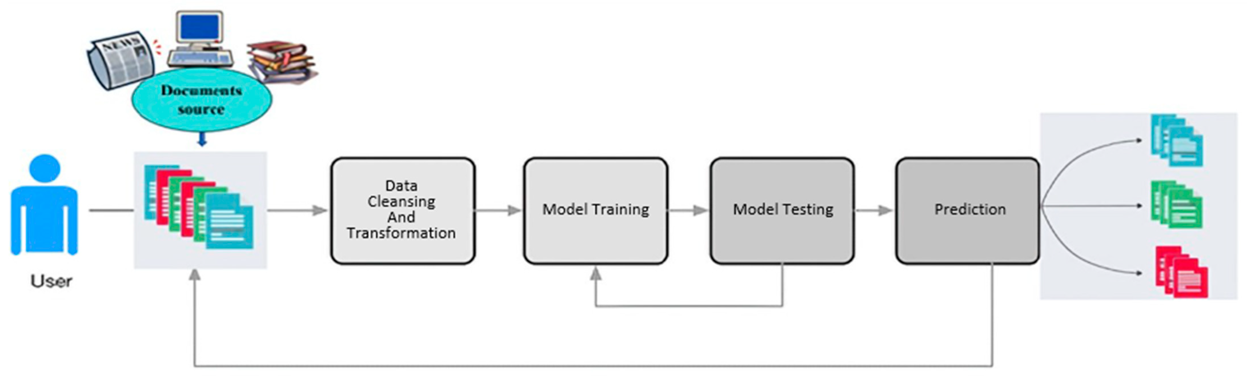
In supervised learning, a computer algorithm trains input data labeled for a specific output. As shown in Figure 1, the model is trained until it can detect the underlying patterns and relationships between the input data and the output labels, enabling it to yield accurate labeling results when presented with never-before-seen data [7]. A user can tag new and old data if the model correctly categorizes it [8]. Classification and regression problems, especially those involving binary classification, are well-suited to supervised learning [8].

The typical approach to evaluating an information retrieval system is distinguishing pertinent and irrelevant documents. Then, document collection and gathering of relevancy scores decide the system’s effectiveness. Although, for example, a researcher may assign zero to irrelevant and one to pertinent documents, the collection and feature extraction process of the documents can affect the system’s effectiveness.

2. Literature Review

Several papers have proved that data preprocessing can help change performance metrics that affect imbalanced classification. Goudjil et al. introduce an innovative active learning method for text categorization, aiming to minimize labeling effort while maintaining classification accuracy by intelligently selecting appropriate samples [9]. Kadhim’s paper evaluates various text preprocessing tools for English text classification, including raw text, tokenization, stop words removal, and stemming; results show that preprocessing enhances feature extraction methods, especially for small threshold values [10]. Mali et al. paper explores the impact of preprocessing steps on text classification, revealing improvements in accuracy in various classifiers, mainly when applied to unstructured data, despite the vast amount of digital information available [11].

Likewise, similar works focused on different subsampling strategies and training size variations to change performance measures. Imberg et al. propose an active sampling strategy that iterates between estimation and data collection with optimal subsamples, guided by machine learning predictions on unseen data [12]. Kumar et al. study addresses challenges in mental health NLP by using the Anno-MI dataset for counseling quality classification. It employs data augmentation to improve reliability, reduce bias, and address data scarcity and imbalance [13]. In transmitter classification applications, Oyedare and Park explored the relationship between training dataset size and classification accuracy, suggesting that users should choose how much training data is required to offer the optimum performance metrics [14].

Three papers focusing on various text classification methodologies can address various classification challenges. First, Li et al. propose a paper that reviews text classification approaches from 1961 to 2021, focusing on traditional models and deep learning. It provides a taxonomy, technical developments, benchmark datasets, comparisons, evaluation metrics, and critical implications [15]. Mubjata et al. review measures the performance of SML and rule-based approaches, presenting open research issues and challenges from nine types of clinical reports, four data sets, two sampling techniques, and nine pre-processing techniques [16]. Finally, Kamath et al. compared the accuracy of four machine learning classifiers and one convolutional neural network on raw and cleaned datasets [17].

Some research articles have proven inefficient and practical approaches to analyzing imbalanced sample difficulties. Kim & Hwang et al. evaluated a combination of seven sample strategies and eight machine learning classifiers on 31 datasets with varying degrees of imbalance and discovered that some sampling procedures could have been more efficient and helped classifier performance. In contrast, others were more successful [18]. Agarwal et al. developed a novel sampling strategy to increase classification task performance and a custom-based sampling method to determine which methods affect the performance [19]. Gaudreault et al. research investigates performance assessment and predictive modeling in machine learning applications dealing with imbalanced domains. It explores metrics and implementations for class-specific performance, aiming to provide recommendations for optimal performance [20].

Researchers conduct trials using various statistical methodologies to aid in evaluating performance measurements. Mishra et al. show Student’s t-test, ANOVA, and ANOVA are statistical methods used to compare means between groups, with ANOVA showing significant differences using multiple comparisons. These methods are crucial for small sample sizes due to outliers [21]. To better display data, Nordmann et al. advocate employing exploratory data analysis techniques such as bar charts, histograms, converting or aggregating data, density plots, and box plots [22]. Aust et al. explores how to translate default priors from linear mixed models to corresponding aggregate analyses in repeated measures ANOVA and paired t-tests [23]. Moscarelli’s paper examines exploratory data analysis (EDA) to describe a comprehensive procedure, including the importation, cleansing, potential transformation, analysis, and subsequent visualization of data to enhance comprehension of its underlying characteristics [24]. Future research may reimplement similar ideas or introduce new methods from this paper. The results demonstrate the efficacy of machine and deep learning algorithms in evaluating various training sizes.

3. Methodology

The dataset is a total of 1000 PDF documents. Five machine learning labels exist (Immune, Problems in China, Risk Factors, Transmission, and Testing). Furthermore, 25% of the PDF documents are open-access COVID-19 research papers from the World Health Organization COVID-19 Downloadable Articles Database to have a positive class [25]. The WHO COVID-19 Downloadable Articles Database supplies free access to open-access documents and includes a bibliography of documents in CSV format.

A user can manually download a specific kind of PDF document from the COVID-19 research database to help serve as a dataset for the positive class. The other 75% of PDF documents are non-related COVID-19 research papers from the PubMed Central database to have a negative class [26]. Both the positive and negative class has papers relevant to biomedical literature. The documents in the positive class are particularly related to COVID-19; however, the negative class includes papers relevant to any medical subject, excluding COVID-19. A user can obtain the PDF documents from PubMed Central using the PubMed Central Open Access Subset, which maintains a repository of open-access paper archives suitable for reproducing research [27]. One user creates the dataset used for the experiment.

Both approaches require using the Python libraries Scikit-learn, NumPy, and Pandas to perform feature engineering, imbalanced classification, and text classification on raw text data [28]. R script and Xpdf command line tools convert all portable document format (PDF) documents into text files in a directory. The goal of combining the text files is to make the classifier’s processing easier. The first approach uses the text files in the MEDFULL folder as the first dataset. The combining process creates two combined text files (such as Immune-pos.txt and Immune-neg.txt) for both positive and negative classes based on a single label. Even though each label has the same number of document or text files, the class has different samples and file sizes.

The methodology’s second approach requires a user to convert the individual raw text files for each labeled in the MedText folder to a CSV file so that the sentences can have the source code automatically annotate keywords based on regular expressions. The keywords are terms based on the data origin close to COVID-19 (such as clinical, isolation, respiratory, disease, spread, PMC, symptomatic, epidemic, endemic, outbreak, quarantine, and others) [29]. The metacharacters and characters associated with regular expressions are best associated with an example like “(?i)(?i:C|c)lincial|(?i:I|i)nfectious|(?i:C|c)ornavirus|(?i:D|d)isease|(?i:C|c|o|O|v|V|i|I|D)|(?i:p|P)ositive|(?i:C|c)ommunity|(?i:C|c)ase(?i:N|n)egative|(?i:A|a)rea|(?i:e|E)pidemic|(?i:E|e)ndemic|(?i:O|o)utbreak|(?i:I|i)solation|(?i:R|r)espiratory|(?i:S|s)pread|PMC|(?i:S|s)ymptomatic”. This regular expression matches characters being words in either all lowercase, all uppercase, or title case format. The regular expression matches terms like disease, Disease, Respiratory, respiratory, COVID-19. The matched terms supplied the label. Next, a script transfers the converted CSV files of each label and positive class to a COVID_ANN folder following the illustration in Figure 2. In the second approach, which entails automatically labeling documents based on regular expressions, we exclude the negative text files depicted in Figure 2 for each label. The No symbol in Figure 2 indicates that files from the negative class are not processed further. This implies that only positive documents undergo consideration for automatic labeling. Below, references to the COVID_ANN dataset refer to a complete collection of the CSV annotated files of the converted raw text documents. First, combine and merge all annotated CSV files from the Immune, Problems in China, and Risk Factors labels to form ‘COVID_Train_Set.csv,’ the Train Subset. Next, users combine and merge all annotated CSV files from the Testing label to create a file called ‘COVID_Dev_Set.csv,’ the Dev Subset. Finally, connect and merge all annotated CSV files from the Transmission label to make the Test Subset file ‘COVID_Test_Set.csv.’ These three subsets or CSV files form ‘Subset Data,’ the second dataset.

3.1. Preprocessing and Labeling

In the first approach of the experiment, a Python script conducts data preprocessing in two phases: noise removal and normalization. Noise removal removes unwanted content from the unstructured text by using the various functions from the NLTK library, such as stopwords, wordnet, WordNetLemmatizer, and word_tokenize. After removing the added noise, normalization helps process the data. A script can concatenate the two negative and positive text files of each label as sentences in a Pandas data frame and then combine them. The Pandas data frame has six columns, excluding the index column, proving the data preprocessing step process. The first step is relevant to extracting raw sentence data. In the second step, the script labels documents with 1s and 0s. The third step removes any punctuation. The fourth step involves tokenizing the sentences. The fifth step involves removing stopwords. The last step involves lemmatizing the words accordingly. All the sentences undergo a noise removal process for better-improved data reading [26].

The string.punctuation module removes all punctuation before tokenization to prevent tokenizing unwanted elements. The word_tokenize function from the NLTK library tokenizes the sentences as a data point. The stopwords module removes stopwords from the tokenized text. Finally, for machine learning models to preprocess unique data, lemmatization (using the WordNetLemmatizer and WordNet modules) must decide the base words of all dataset words and execute them in the machine learning model before the feature extraction process.

Table 1. Number of Samples for Each Label After Data Conversion.

Label	Number of Rows or Sentences in CSV File
Immune	46,727
Problems in China	47,154
Risk Factors	23,666
Testing	99,367
Transmission	43,952

shows the number of samples relevant to each label. The number of rows corresponds to the number of sentences or samples after converting the text files from MedText data to a Pandas data frame and CSV file for each label. For example, combining [label]-neg.csv and [label]-pos.csv results in a [label].csv. The machine learning model processes each label with a unique CSV file with different sentences as rows. The experiment’s first approach may have affected each classifier’s performance and imbalanced sampling technique from their intended purposes.

After processing text files for each specific label from the MEDFULL data, the method displays three different subsets in separate CSV files named COVID_Train_Set.csv, COVID_Dev_Set.csv, and COVID_Test_Set.csv.

Table 2. Number of Samples for Each Subset After Data Conversion.

Subset	Number of Samples or Sentences in CSV File
Train Set	50,427
Dev Set	14,327
Test Set	16,256

displays the number of samples or sentences from rows of CSV files relevant to each subset. After converting the text files to a Pandas data frame or a CSV file, the method considers the sentences or samples as the number of remaining rows. Each subset has a different CSV file with different sentences and rows.

The second approach of the experiment does not perform data preprocessing by using the NLTK library on the sentences. The CSV file has a ‘sentence’ column with the raw text by each sentence line, as shown in

Table 3. Labeling using Keyword Matching via Regular Expressions.

	Sentence	Label	Data	Regex
0	Research Letters	0	N/A	False
1	Table 1. Clinical characteristics of 604 patients with systemic lupus erythematosus with and without COVID-19 a Mean (standard deviation).	1	Clinical	True
2	SLE patients with COVID-19 reported a lower frequency of social isolation.	1	COVID-19	True
3	Secondary AA can be caused by infections, drugs, or various diseases.	1	Disease	True

. A user annotates the positive documents from each of the five labels. The CSV files automatically annotate the documents using regular expressions. First, annotate the documents by using regular expressions. Suppose a sentence in the sentence column has data that matches the regular expression pattern. In that case, the user can assign the number one in the ‘label’ column, showing it is positive, as shown in

Table 4. Number of Samples for Each Label Based on Subsampling.

Label	Percentage	Iteration	Number of Samples
Immune	5%	1	2336
Problems in China	10%	2	4715
Risk Factors	40%	8	9466
Testing	95%	19	94,398
Transmission	20%	4	17,580
Immune	25%	5	11,681
Transmission	30%	6	39,556

. If the sentence in the sentence column has data that does not match the regular expression used to automatically label the sentences, as shown in Table 3, the user assigns it with zero. Regular expressions extract specific keywords from each sentence’s ‘Data’ column. The ‘Regex’ column shows a Boolean expression if the regular expression matches the sentence column of a particular row, as shown in Table 4 [26]. The second approach of the experiment supplies a more authentic performance that shows imbalanced sampling techniques and classifiers work effectively.

3.2. Subsampling and Training Size Variation

Subsampling the number of samples or sentences would affect the classifier’s performance. Therefore, the subsampling intends to use only a certain number of sentences based on an interval. Subsampling requires dividing the samples or sentences of positive and negative data frames by 5% and 10% intervals. Depending on the interval percentage, the Python script selects a specific number of samples from the positive and negative data frames and labels columns to subsample the data. The selection of samples starts from zero to a specific number of samples based on percentage or interval. Finally, the script combines positive and negative data frames based on intervals for the machine learning model to perform subsampling.

Mathematical functions calculate the number of samples based on the iterations or subsample size used by the machine learning model after processing the combined CSV files or data frames for each label’s positive and negative classes, as detailed in Table 4. Again, the original MEDFULL data is necessary for this computation. The subsample size ranges from 5% to 100%, with intervals of 10%, 15%, 20%, and others, as shown in Table 3 for the first approach [26].

Table 5. Number of Samples for Each Subset Based on Subsampling.

Subset	Percentage	Iteration	Number of Samples
Train Set	10%	1	5042
Test Set	20%	2	3251
Dev Set	30%	3	4876
Dev Set	40%	4	6502
Train Set	90%	9	45,384
Dev Set	70%	7	10,028
Train Set	60%	6	30,256

shows the sample sizes based on the number of iterations or subsample sizes; the machine learning model calculates after processing the combined CSV files or data frames for each subset’s positive and negative classes. It displays the intervals used in the second approach, ranging from 10% to 100%, including 20%, 30%, 40%, and others. The first approach uses 20 subsample iterations, while the second uses 10.

Each classifier has specific parameters to execute during each iteration and subsampling size. The machine learning model sequentially adjusts the train split size to 17%, 33%, 50%, 67%, and 83% for each iteration, with the test split size being the remaining 100% minus the train split size for the first approach. The second approach uses a constant 50% training and testing size relevant to every iteration.

When subsampling occurs on the data from the first approach, iterations 1 to 13 or a subsample size initially beginning 5% to 65% increases or decreases the performance variation for all classifiers and imbalanced sampling techniques. Once iteration 13 is reached, the machine learning models provide the best or worst performance depending on each imbalanced sampling technique and classifiers. When the second approach involves subsampling, increasing the subsampling size from 10% to approximately 90% or 100% significantly improves the performance of all imbalanced sampling techniques and classifiers. The subsampling size of 50% did supply the worst performance for all imbalanced sampling techniques and classifiers.

3.3. Classification Tasks

The method uses five machine learning classifiers: Random Forest, Naïve Bayes, Support Vector Machine, XGBoost, and Decision Tree [18,19,20]. The machine learning classifiers, including the Naive Bayes module, the linear model module, the tree module, and the ensemble module, require modules from the Scikit-learn library and the XGBoost library to run. The linear model module in Scikit-learn executes classifiers that evaluate variables that show a linear relationship. XGBoost is a machine-learning library that uses gradient-based optimization, regularization methods, and weighted quantile sketch to manage massive datasets effectively. The tree module in Scikit-learn supplies tree-based models, a machine learning model that evaluates variables that show a decision-based arrangement. The Scikit-learn library’s ensemble module combines various base models of the Random Forest classifier for more efficiency. Finally, the Naïve Bayes module runs three kinds of machine learning classifiers of Naïve Bayes classifiers [26].

When there is a distortion from the allocation of classes in training data toward one class, the Imbalanced-learn library in Python can help solve imbalanced classification problems. This library has both Oversampling and Undersampling modules, with the Oversampling module supplying the SMOTE and RandomOverSampler methods and the Undersampling module featuring RandomUnderSampler, TomekLinks, and NearMiss functions. The RandomOverSampler method has settings with a random state of 42. At the same time, the parameters of the RandomUnderSampler are an arbitrary state of 42 and true replacement.

Feature Extraction involves using the TfidfVectorizer, a Scikit-learn feature extraction method that converts raw text into TF-IDF features to decide the relevance of words in a document or corpus and perform feature engineering and data preprocessing tasks. The TfidfVectorizer has an n-gram range of (1, 2) for all machine learning models. It shows that when deconstructing raw sentence data, it will include single and two-grams (pairs of consecutive words) depending on the label. In addition, the TfidfVectorizer uses lemmatized or raw sentence data from all sentences to create matrices for each classifier and sampling technique, which can either negate or promote an imbalance issue.

When subsampling is applied, it progressively enhances classifier performance until a specific subset is reached, achieving optimal performance metrics such as precision, recall, AUROC, and accuracy, after which further increases may lead to a decline. Applying variation in training size can lead to sporadic results in precision and recall. For instance, if the training size is 67% with a testing size of 33% from a subsampling size of 5%, the precision would be above 90% and recall between 35% to 45%. Now, if the training size is 33% and the testing size is 67% from the subsampling size, the precision would be around 30% to 35%, and recall between 90% to 100%. However, the expected performance for each classifier would remain the same even if it had a different subsampling technique. This means that Logistic Regression could have a lower precision score of 31% or a higher precision score of 94% depending on the training size, which would be lower than other classifiers.

3.4. Machine Learning Classifiers

The types of models used in this experiment are statistical (Logistic Regression), tree-liked (Decision Tree and Random Forest), ensemble learning (XGBoost and Random Forest), and probabilistic model (Naïve Bayes). Logistic Regression is a classifier that decides the likelihood of predicting that an instance belongs to a certain class as its main objective. Logistic regression models the likelihood of an output in terms of input characteristics, as opposed to linear regression, which predicts continuous values [30]. While it does not perform direct statistical classification, selecting a cutoff value can be employed to construct a classifier. This method commonly assigns inputs with probabilities above the cutoff to one class and those below the cutoff to the other in creating binary classifiers [30].

Predicting the category or class of a given instance is the aim of the probabilistic machine learning method Multinomial Naïve Bayes classifier based on Bayes’ theorem. It works well with data with characteristics that indicate discrete frequencies or counts of occurrences in various natural language processing (NLP) applications because it can compute the probability distribution of text data [31]. XGBoost is a machine learning algorithm that harnesses the predictions of weak models, typically decision trees, to construct a robust predictive model. Regression, classification, and ranking issues are among its common applications. Constructing a powerful classifier from a set of feeble classifiers is the aim. GPU support, a specialized data structure, goals, loss functions, cross-validation support, and APIs are all features of XGBoost [32]. The Random Forest classifier is a meta-estimating classifier that uses averaging to enhance prediction accuracy and address over-fitting. To accomplish this, the algorithm fits several decision tree classifiers on various subsamples of the dataset. It constructs these trees by randomly training them on different subsets. Subsequently, these trees participate in a “voting” process to determine the final prediction, with most trees determining the outcome. Random Forests mitigate overfitting and enhance forecast accuracy by aggregating the information of several trees [33]. Decision Tree classifier builds a flowchart-like tree structure where each internal node denotes a test on an attribute, each branch represents an outcome of the test, and each leaf node (terminal node) holds a class label [34]. Decision trees have a hierarchical structure of root nodes, branches, leaf nodes, and internal nodes. Decision trees are considered non-parametric; they make no spatial distribution or classifier structure assumptions and can handle numerical and categorical variables [35].

The features encompass sentences that undergo preprocessed or non-preprocessed treatment to eliminate and filter out undesired elements using conventional preprocessing techniques. We alternated these features to assess their impact on the performance of each classifier and imbalanced sampling technique. Additionally, it is necessary to vectorize these features for use by any machine learning classifier in the methodology. The labels consist of positives (1 s) and negatives (0 s) for each respective class of the dataset. The classifiers and imbalanced sampling techniques are all implemented similarly. The only factors that change the performance of each classifier are vectorization, training or testing size, and subsampling size. Before running the machine learning model, balance the sampling of classifiers and imbalanced sampling techniques. When employing an imbalanced sampling technique, the features undergo resampling based on the majority class (negative) and the minority class (positive). The machine learning models execute XGBoost, Naïve Bayes, and Decision Tree classifiers with default parameters. However, the machine learning models have changed parameters for Random Forest and Logistic Regression to optimize performance, considering the small size of the dataset. Logistic Regression is potentially biased to undersampling techniques used in this experiment that could have contributed to improved performance than other classifiers [36].

XGBoost has the fastest execution as an ensembling learning classifier, enabling it to supply the highest performance shown in this study. Random Forest classifier uses ensemble learning but takes the longest to execute and to supply a different performance result from other classifiers that are faster in execution. For detecting discrete features in text classification, it is suitable to use Multinomial Naïve Bayes. Logistic Regression classifier depends on binary variables that make it suitable for any binary classification problem. This study uses binary classification instead of multiclass classification, making the Logistic Regression classifier suitable for the hypothesis associated with this experiment. The Decision Tree Classifier promotes swift execution, considering its efficacy for binary and multiclass tasks. The Decision Tree classifier is the primary classifier evaluated in the machine learning model.

3.5. Statistical Analysis

For statistical analysis, the R programming language requires the following packages: the tidyverse package collection, modelr package, rstatix package, ggpubr package, hexbin package, stats package, and reshape package. Based on the concepts of tidy data, the Tidyverse collection has specific packages such as dplyr, ggplot2, tidyr, readr, purrr, tibble, and more to visualize and preprocess data [24].

A statistician can use the tidyverse collection for exploratory data analysis, notably tibble and ggplot2. In keeping columns, rows, and variable types, a tibble differs from a conventional data frame in a more readable way. The ggplot2 package uses graphics grammar to map visual components to variables and arrange them on a plot to create a wide range of visualizations [26].

The tibble package has the as_tibble function, the stats package has the pairwise_t_test function, and the rstatix package has functions such as get summary stats, anova_test, stat_pvalue_manual, and ggboxplot for hypothesis testing. The as_tibble function changes data frames to the tibble format. The pairwise_t_test function uses a paired t-test to assess the differences between two groups to evaluate a hypothesis. The get_summary_stats function produces summary statistics for a dataset, such as the central tendency, dispersion, quartiles, and interquartile ranges. Finally, the ANOVA function uses analysis of variance (ANOVA) to decide whether a statistically significant difference exists between groups [22,37].

In contrast, the F-value evaluates the variation within and between populations. This function handles showing the degrees of freedom represented by the numerator and denominator for ANOVA to compute a F-value of the Regression Mean Square divided by Mean Squared Error [38]. Bonferroni correction mitigates the possibility of bias introduced by concurrently conducting too many comparisons. The R function stat_pvalue_manual computes and shows the p-value for a hypothesis test based on two groups or conditions from a T-test, ANOVA, and Bonferroni correction [39]. Finally, the ggboxplot function generates box plot graphs that supply a visual depiction from rstatix package functions.

4. Experiment and Results

The machine learning models evaluate performance metrics from five labels specified in Section 3.1, using the Train, Dev, and Test Subsets. In the first approach, a script organizes the COVID_Iterations.csv file with specific columns, including “Label”, “Sampling”, “Technique”, “Classifier”, “Test Split Size”, “Train Split Size”, “Iteration”, “Subsampling Size”, “Precision”, “Recall”, “AUROC”, and “Accuracy”. The Label column specifies the five categories: Immune, Risk Factors, Problems in China, Testing, and Transmission. The Sampling column finds three types of sampling: Imbalanced, Oversampling, or Undersampling [39,40]. The Technique column specifies five sampling methods: Synthetic Minority Oversampling Technique (SMOTE), Random Undersampling (RUS), Random Oversampling (ROS), TomekLinks, and NearMiss [18,39]. SMOTE [40] uses a fake point to create a vector between an existing data source and one of its peers, avoiding overfitting. RUS technique replaces specific data from the majority class to create an even or compacted distribution. In contrast, ROS substitutes random samples from minority classes to create a more evenly distributed training set [41].TomekLinks are pairs of events that occur near one another but take different routes, amplifying the two groups by removing dominant members, and NearMiss is a controlled under-sampling technique that replaces members of the dominant class with negative samples to improve space and reduces data loss [42].

Then, the Python script stores the scores in the CSV files with the designated columns based on the output formatting, where the Scikit-learn library’s metrics module supplies four specific scores for classifiers: precision, recall, AUROC, and accuracy. The script categorizes scores without a sampling technique and method as ‘Imbalanced’ in the Sampling and Technique columns. The Classifier column can specify five classifiers: Logistic Regression, XGBoost, Decision Tree, Naïve Bayes, and Random Forest. Subtracting one from The Train Split Size column is 100% remaining from the Test Split Size. The Iteration and Subsample columns can range from 1 to 20 intervals by 5% up to 100% for the first approach or 1 to 10 intervals by 10% up to 100% for the second approach. Precision, Recall, AUROC, and Accuracy columns can range from 0% to 100% in decimal values [26].

The script stores the scores in NumPy arrays each time a classifier executes, depending on the sampling method, sampling technique, test split size, train split size, subsampling iteration, and subsample size. After running the classifiers based on one set of train and test split sizes, the Python script appends the scores to the earlier score in each NumPy array.

Similarly, the COVID_Subset_Iterations.csv file of the second approach defines columns such as “Subset”, “Other Subset”, “Sampling”, “Technique”, “Classifier”, “Iteration”, “Precision”, “Recall”, “AUROC”, and “Accuracy”. These files record the evaluation metrics for each model, sampling method, and iteration, enabling analysis and comparison of the results.

Each classifier has specific parameters to execute during each iteration and subsampling size. The machine learning model sequentially adjusts the train split size to 17%, 33%, 50%, 67%, and 83% for each iteration, with the test split size being the remaining 100% minus the train split size. The first approach employs five different training and testing split sizes, while the second uses a fixed training and testing size of 50%.

The train test split module from the Scikit-learn library performs training size variation. The Scikit-learn model selection function is a set of tools used for feature engineering on models. The train test split module, included in the Scikit-learn package, is valuable for splitting a dataset into two or more pieces for training and testing machine learning models. When conducting the train test split module during each subsampling iteration of the classifier, a user can specify the number of samples from each label to decide how closely the positive and negative classes match.

4.1. Results from MEDFULL Data

The MEDFULL data collection involves five labels (Immune, Problems in China, Risk Factors, Testing, and Transmission). This first approach uses data preprocessing techniques and manually assigns the document based on the content to positive and negative classes in our experiment and has shown not to have an imbalanced class issue [26].

Table 6. Highest Performance Metrics from COVID Iterations.

Label	Technique 1	Classifier 1	Test Split Size	Train Split Size	Iteration	Precision	Recall	AUROC	Accuracy
Immune	NM	LR	0.67	0.33	13	1	0.557233	0.778617	0.602797
Problems in China	NM	RF	0.67	0.33	13	1	0.618273	0.809136	0.691296
Immune	NM	NB	0.67	0.33	13	0.999266	0.584622	0.791048	0.64464
Risk Factors	NM	XG	0.67	0.33	13	0.998252	0.620652	0.808094	0.69405
Problems in China	NM	DT	0.67	0.33	13	0.996917	0.578932	0.78391	0.635826

¹ The technique used is only relevant to Undersampling techniques. Full words for abbreviations: NM—NearMiss, LR—Logistic Regression, RF—Random Forest, NB—Naïve Bayes, XG—XGBoost, DT—Decision Tree.

shows the highest precision at 100% from an iteration of 13 or 65% subsampling size. The precision scores are between 99.6% to 100%. The recall scores are around 55% up to 85%. It shows that the best subsample size at 65%, or iteration 13 when the test split size is at 67% or 83%, and the train split size is at 17% to 33%, provides only sufficient data to get the highest performance from the classifiers and imbalanced sampling techniques.

Table 7. Lowest Performance Metrics from COVID Iterations.

Label	Technique 1	Classifier 1	Test Split Size	Train Split Size	Iteration	Precision	Recall	AUROC	Accuracy
Testing	NM	LR	0.5	0.5	13	0.093478	0.014517	0.436867	0.436867
Testing	NM	XG	0.5	0.5	13	0.120879	0.00945	0.470361	0.470361
Testing	NM	NB	0.5	0.5	13	0.139394	0.013046	0.466251	0.466251
Transmission	NM	DT	0.5	0.5	13	0.188406	0.02054	0.466834	0.466834
Testing	NM	RF	0.5	0.5	13	0.142857	0.01	0.47495	0.474562

¹ The technique used is only relevant to Undersampling techniques. Full words for abbreviations: NM—NearMiss, LR—Logistic Regression, RF—Random Forest, NB—Naïve Bayes, XG—XGBoost, DT—Decision Tree.

shows the lowest precision and recall scores found from an iteration of 13 or 65% subsampling size when the test and train split sizes are 50%. The results demonstrate that iteration 13 has sporadic results.

Table 8. Average Performance Metrics Based on Label for MEDFULL Data.

Label	Precision	Recall	AUROC	Accuracy
Immune	0.73670	0.70131	0.67559	0.66176
Problems in China	0.66540	0.63147	0.67900	0.66442
Risk Factors	0.73396	0.72982	0.68216	0.67627
Testing	0.72046	0.68546	0.67397	0.65945
Transmission	0.75239	0.69499	0.67528	0.66179

summarizes the label’s average scores regardless of sampling method and technique, classifier, train split size, test split size, iteration, and subsampling size. Again, Risk Factors supply the best scores, while the Testing label provides the worst scores.

Table 9. Average Performance Metrics Based on Classifier for MEDFULL Data.

Classifier	Precision	Recall	AUROC	Accuracy
Logistic Regression	0.69871	0.65753	0.64769	0.63780
Decision Tree	0.71524	0.68682	0.67128	0.65943
Naïve Bayes	0.72550	0.69172	0.68216	0.66924
XGBoost	0.73302	0.70026	0.68971	0.67609
Random Forest	0.73641	0.70673	0.69517	0.68113

summarizes each classifier’s average precision, recall, AUROC, and accuracy scores regardless of sampling method, sampling technique, label, train split size, test split size, iteration, and subsampling size. Again, the XGBoost classifier supplies the best scores, while the Logistic Regression classifier supplies the worst.

Table 10. Average Performance Metrics Based on Sampling for MEDFULL Data.

Sampling	Precision	Recall	AUROC	Accuracy
Imbalanced	0.73295	0.69637	0.66433	0.66619
Oversampling	0.71301	0.68496	0.68092	0.66251
Undersampling	0.68846	0.68846	0.67902	0.66574

summarizes the sampling method’s average precision, recall, AUROC, and accuracy scores regardless of classifier, sampling technique, label, train split size, test split size, iteration, and subsampling size. Again, the scores from imbalanced data outperform the other types of sampling methods (Oversampling and Undersampling).

Table 11. Average Performance Metrics Based on Technique for MEDFULL Data.

Technique	Precision	Recall	AUROC	Accuracy
Imbalanced	0.73295	0.69636	0.66432	0.66618
NearMiss	0.71225	0.68521	0.67541	0.65667
ROS	0.71283	0.68693	0.68151	0.66313
RUS	0.72433	0.68984	0.68834	0.66945
SMOTE	0.71319	0.68299	0.68026	0.66189
TomekLinks	0.73521	0.69033	0.67333	0.67109

summarizes the average sampling technique’s precision, recall, AUROC, and accuracy scores regardless of sampling method, label, classifier, train split size, test split size, iteration, and subsampling size. When the machine learning models use imbalanced sampling techniques, they have shown slight effectiveness than simply running machine learning models on the imbalanced dataset. TomekLinks has the best scores in comparison to other imbalanced sampling techniques. NearMiss has the worst scores.

Table 12. t-test Statistics of Precision Based on Classifiers for MEDFULL Data.

Metric	Group 1 1	Group 2 1	p	p.signif 1	p.adj 1	p.adj.signif 1
Precision	DT	LR	1.09 × 10−3	**	1.09 × 10−2	*
Precision	DT	NB	4.26 × 10−2	*	4.26 × 10−1	ns
Precision	LR	NB	1.21 × 10−7	****	1.21 × 10−6	****
Precision	DT	RF	2.89 × 10−5	****	2.89 × 10−4	***
Precision	LR	RF	9.85 × 10−14	****	9.85 × 10−13	****
Precision	NB	RF	3.11 × 10−2	*	3.11 × 10−1	ns
Precision	DT	XG	4.44 × 10−4	***	4.44 × 10−3	**
Precision	LR	XG	1.25 × 10−11	****	1.25 × 10−10	****
Precision	NB	XG	0.137	ns	1.00	ns
Precision	RF	XG	0.503	ns	1.00	ns

¹ The classifiers are compared based on 3000 observations. Full words for abbreviations: LR—Logistic Regression, RF—Random Forest, NB—Naïve Bayes, XG—XGBoost, DT—Decision Tree, ns—non-significance level. ns means p > 0.05, * means p ≤ 0.05, ** means p ≤ 0.01, *** means p ≤ 0.001, and **** means p ≤ 0.0001. p.signf means the significance level of p-values, p.adj means adjusted p-value, and p.adj.signif means the significance level of the adjusted p-value.

displays the ANOVA t-test results for classifiers based on precision. The p-values represent the statistical significance of the variations in accuracy between algorithm pairings. Significant variations (****) in accuracy between Decision Tree and Naive Bayes, Decision Tree and Random Forest, Decision Tree and Random Forest, Logistic Regression and XGBoost, and Logistic Regression and XGBoost are among the noteworthy results. The adjusted p-values show that these significant differences hold even after correcting for multiple comparisons. On the other hand, several comparisons, such as Random Forest with XGBoost, Naive Bayes with Random Forest, and Random Forest with XGBoost, have p-values over the standard cutoff of 0.05 and do not demonstrate any discernible changes.

The ANOVA t-test of classifiers based on recall is shown in

Table 13. t-test Statistics of Recall Based on Classifiers for MEDFULL Data.

Metric	Group 1 1	Group 2 1	p	p.signif 1	p.adj 1	p.adj.signif 1
Recall	DT	LR	6.33 × 10−8	****	6.33 × 10−7	****
Recall	DT	NB	3.65 × 10−1	ns	1.00	ns
Recall	LR	NB	2.72 × 10−10	****	2.72 × 10−9	****
Recall	DT	RF	2.32 × 10−4	***	2.32 × 10−3	**
Recall	LR	RF	1.08 × 10−19	****	1.08 × 10−18	****
Recall	NB	RF	5.52 × 10−3	**	5.52 × 10−2	ns
Recall	DT	XG	1.30 × 10−2	*	1.30 × 10−1	ns
Recall	LR	XG	3.06 × 10−15	****	3.06 × 10−14	****
Recall	NB	XG	1.14 × 10−1	ns	1.00	ns
Recall	RF	XG	2.31 × 10−1	ns	1.00	ns

¹ The classifiers are compared based on 3000 observations. Full words for abbreviations: LR—Logistic Regression, XG—XGBoost, DT—Decision Tree, RF—Random Forest, ns—non-significance level. ns means p > 0.05, * means p ≤ 0.05, ** means p ≤ 0.01, *** means p ≤ 0.001, and **** means p ≤ 0.0001. p.signf means the significance level of p-values, p.adj means adjusted p-value, and p.adj.signif means the significance level of the adjusted p-value.

. The p-values reflect the statistical significance of differences in recall between the algorithm pairs. Several noteworthy findings emerge vital statistical significance (****) is observed in the comparisons between Decision Tree and Logistic Regression, Decision Tree and Naive Bayes, Logistic Regression and Random Forest, Decision Tree and Random Forest, Logistic Regression and XGBoost, and Logistic Regression and XGBoost. These results remain significant even after adjusting for multiple comparisons, indicated by the adjusted p-values. Conversely, some comparisons, such as Naive Bayes with Random Forest and Naive Bayes with XGBoost, show no significant differences, as evidenced by p-values above the conventional threshold of 0.05.

The graph in Figure 3, titled ‘MEDFULL—Precision & Classifier’, shows an F-value of 18.14 with an overall p-value less than 0.0001, meaning a slight variation of sample means between the two groups. Logistic Regression has lower values and the lowest outlier distinctively from other classifiers in this box plot. The Logistic Regression classifier has a significant value, given that it has lower importance than other classifiers of precision scores. XGBoost has two non-significant values meaning the performance of the XGBoost classifier is closely like different classifiers (particularly Naive Bayes and XGBoost). Logistic Regression has a significant level than other classifiers.

The ‘MEDFULL—Recall & Classifier’ graph shows an F-value of 24.64, which offers a slight variation of sample means based on all classifiers. Again, the recall scores differed more considerably than the same precision (categorical variable). Furthermore, in this case, Logistic Regression has shown lower values in the boxplot to justify its p-value significance, like precision scores. In this figure, Naïve Bayes has the most closely non-significant papers in various groups of classifiers. Again, Logistic Regression has the lowest p-values that show a highly significant level in the p-value column.

The ‘MEDFULL—Precision & Sampling’ graph displays slight variations in all box plots between the two groups, with an F-value of 27.64 and an overall p-value less than 0.0001. In this figure, they are all significant when comparing each sampling method, and Oversampling supplies a higher significance level than other methods.

The graph titled ‘MEDFULL—Recall & Sampling’ shows an exceptionally low F-value of 2.46, which proves poor variation between the groups. The overall p-value of 0.086, meaning there is little or no significance when comparing two groups against each other. This figure provided Imbalanced when compared with Oversampling supply, a significantly low level of 0.0268 that cannot deny a null hypothesis. Other comparisons are insignificant, meaning the groups have little or non-existent difference.

The ‘MEDFULL—Precision & Technique’ graph shows an F-value score of 7.19 and an overall p-value less than 0.0001, meaning all sampling techniques and Imbalanced data will partially have differences in performance metrics compared to other groups. However, every sampling technique supplies non-significant and significant results compared to other groups.

The ‘MEDFULL—Recall & Technique’ graph shows an F-value of 1.25 and a p-value of 0.28, meaning there is no or slight variation among the sample means for recall scores. The only comparison of a sampling technique is significant with Imbalanced and SMOTE at p-value at 0.0245. Other comparisons are insignificant.

The ROC curves shown in Figure 4 show the performance of different classifiers depending on the training size, as depicted in Figure 4. The Naïve Bayes has the highest AUC values in all the graphs, from 0.74 to 0.78. Logistic Regression and Random Forest have the second highest values between 0.72 to 0.77. Decision Tree and XGBoost performed similarly at 0.66 and 0.70 when the training size was 16% and 33%. Decision Tree has the second lowest performance of 0.72 and XGBoost has the most inferior performance of 0.71.

Figure 5 shows precision and recall in different facets that compare each sampling technique for MEDFULL data. These facets show that all imbalanced sampling processes and imbalanced data have a similar performance, which does not address the imbalanced problem.

Figure 6 shows a scatter plot of precision and recall in a two-dimensional graph comparing the MEDFULL data sampling technique. The MEDFULL data has more observations for analysis of the performance metrics from CSV rather than Subset data. However, the scatter plot shows that the Imbalanced data performs similarly to other imbalanced sampling techniques.

Figure 7 shows a heatmap of precision and recall for MEDFULL data. Again, the MEDFULL data shows much variability due to more scores and observations. In this heatmap, the highest values are when the recall and precision are around 60%. In this heatmap, even with imbalanced sampling techniques, the classifiers supply the lowest recall and precision scores compared to the Subset data.

4.2. Results from Subset Data

The Subset data collection involves three subsets (Train Set, Dev Set, and Test Set). This second approach uses regular expressions to decide whether a sentence matches a keyword and label it positive or negative. The Subset data collection has addressed the imbalanced issue [26].

Table 14. Highest Performance Metrics from Subset Iterations.

Subset	Other Set	Technique 1	Classifier 1	Iteration	Precision	Recall	AUROC	Accuracy
Train_Set	Test_Set	ROS	XG	9	0.991202	0.936199	0.961843	0.961836
Train_Set	Test_Set	ROS	RF	9	0.991104	0.939023	0.963742	0.963584
Train_Set	Test_Set	ROS	LR	10	0.99074	0.935225	0.96111	0.961088
Train_Set	Test_Set	ROS	NB	10	0.990414	0.93441	0.960697	0.96059
Train Set	Test Set	ROS	DT	10	0.990303	0.9352	0.96712	0.96181

¹ This table only shows statistics related to Random Over Sampling. Abbreviations for Full terms: NM—NearMiss, XG—XGBoost, RF—Random Forest, LR—Logistic Regression, NB—Naïve Bayes, DT—Decision Tree, ROS—Random Over Sampling.

shows that the highest scores can be possible when the iteration is 9 or 10, or the subsample size is 90% or 100%. Therefore, the machine learning models obtain the best scores from Subset data by utilizing 90% and 100% of the dataset.

Table 15. Lowest Performance Metrics from Subset Iterations.

Subset	Other Set	Technique 1	Classifier 1	Iteration	Precision	Recall	AUROC	Accuracy
Train_Set	Test_Set	NM	LR	5	0.541509	0.988519	0.597201	0.58692
Train_Set	Test_Set	NM	DT	5	0.578896	0.989391	0.647256	0.641251
Train_Set	Test_Set	NM	XG	5	0.594941	0.993838	0.665787	0.662264
Train Set	Test Set	NM	RF	5	0.598006	0.982636	0.66621	0.663715
Train Set	Test Set	RUS	NB	6	0.676887	0.989792	0.762975	0.760883

¹ This table only shows statistics related to undersampling techniques. Abbreviations for Full terms: NM—NearMiss, LR—Logistic Regression, DT—Decision Tree, XG—XGBoost. RF—Random Forest, and NB—Naïve Bayes, RUS—Random Under Sampling.

shows that the lowest scores are possible when the dataset has a 50% and 60% subsampling size or iterations of 5 and 6. The results show that only half of the samples from the Train Set, Dev Set, and Test Set can obtain the lowest scores from the dataset.

Table 16. Average Performance Metrics Based on Label for Subset Data.

Other Set	Precision	Recall	AUROC	Accuracy
Dev Set	0.87700	0.89124	0.90969	0.93094
Test Set	0.88963	0.92072	0.91150	0.92239

shows the average scores from the Test Set supply better in the precision, recall, and AUROC columns. However, Dev Set was only superior in the accuracy scores column.

Table 17. Average Performance Metrics Based on Classifier for Subset Data.

Classifier	Precision	Recall	AUROC	Accuracy
Logistic Regression	0.87255	0.90081	0.90472	0.92019
Decision Tree	0.87802	0.89721	0.90504	0.92357
Naïve Bayes	0.88158	0.90666	0.91178	0.92795
XGBoost	0.88811	0.90934	0.91281	0.92854
Random Forest	0.89632	0.91591	0.91861	0.93306

summarizes each classifier’s average precision, recall, AUROC, and accuracy scores regardless of other categories. Again, Logistic Regression has the worst performance as a classifier, while Random Forest has the best performance.

Table 18. Average Performance Metrics Based on Sampling for Subset Data.

Sampling	Precision	Recall	AUROC	Accuracy
Imbalanced	0.84944	0.85076	0.89556	0.93002
Oversampling	0.92292	0.96919	0.93650	0.93646
Undersampling	0.89270	0.92173	0.91198	0.92116

summarizes the average precision, recall, AUROC, and accuracy scores for each type of sampling regardless of other categories. Again, the Oversampling methods outperform the imbalanced data and Undersampling methods.

All imbalanced sampling techniques perform more effectively than imbalanced data in three types of metrics (precision, recall, and AUROC), excluding accuracy, as shown in

Table 19. Average Performance Metrics Based on Technique for Subset Data.

Technique	Precision	Recall	AUROC	Accuracy
Imbalanced	0.84944	0.85076	0.89556	0.93002
NearMiss	0.88845	0.93946	0.89687	0.89649
ROS	0.92292	0.96919	0.93650	0.93646
RUS	0.89881	0.94409	0.90935	0.90915
SMOTE	0.92631	0.97026	0.93950	0.93950
TomekLinks	0.87189	0.86592	0.90840	0.93632

. The second approach of the method using regular expressions that match keywords to label documents in values of one and zero has helped address the imbalanced class problem from the average performance metrics provided.

Table 20. t-test Statistics of Precision Based on Classifiers for Subset Data.

Metric	Group 1 1	Group 2 1	p	p.signif 1	p.adj 1	p.adj.signif 1
Precision	DT	LR	0.6380	ns	1.000	ns
Precision	DT	NB	0.7600	ns	1.000	ns
Precision	LR	NB	0.4380	ns	1.000	ns
Precision	DT	RF	0.1160	ns	1.000	ns
Precision	LR	RF	0.0414	*	0.414	ns
Precision	NB	RF	0.2050	ns	1.000	ns
Precision	DT	XG	0.3860	ns	1.000	ns
Precision	LR	XG	0.1810	ns	1.000	ns
Precision	NB	XG	0.5740	ns	1.000	ns
Precision	RF	XG	0.4810	ns	1.000	ns

¹ The classifiers are compared based on 120 observations. Full words for abbreviations: LR—Logistic Regression, XG—XGBoost, DT—Decision Tree, RF—Random Forest, ns—non-significance level. ns means p > 0.05, * means p ≤ 0.05, ** means p ≤ 0.01, *** means p ≤ 0.001, and **** means p ≤ 0.0001. p.signf means the significance level of p-values, p.adj means adjusted p-value, and p.adj.signif means the significance level of the adjusted p-value.

shows the Logistic Regression and Random Forest comparison in Group 1 and Group 2 yields a p-value of 0.0414, marked with an asterisk (*) showing significance at the 0.05 level. However, this significance disappears after adjusting for multiple comparisons (p.adj), suggesting that the observed difference may be due to chance. The results show no statistically significant differences in precision between Group 1 and Group 2.

Table 21. t-test Statistics of Recall Based on Classifiers for Subset Data.

Metric	Group 1 1	Group 2 1	p	p.signif 1	p.adj 1	p.adj.signif 1
Recall	DT	LR	0.7320	ns	1.000	ns
Recall	DT	NB	0.3700	ns	1.000	ns
Recall	LR	NB	0.5790	ns	1.000	ns
Recall	DT	RF	0.0765	ns	0.765	ns
Recall	LR	RF	0.1530	ns	1.000	ns
Recall	NB	RF	0.3800	ns	1.000	ns
Recall	DT	XG	0.2500	ns	1.000	ns
Recall	LR	XG	0.4190	ns	1.000	ns
Recall	NB	XG	0.8000	ns	1.000	ns
Recall	RF	XG	0.5330	ns	1.000	ns

¹ The classifiers are compared based on 120 observations. Full words for abbreviations: LR—Logistic Regression, XG—XGBoost, DT—Decision Tree, RF—Random Forest, ns—non—non-significance level. ns means p > 0.05, * means p ≤ 0.05, ** means p ≤ 0.01, *** means p ≤ 0.001, **** means p ≤ 0.0001. p.signf means the significance level of p-values, p.adj means adjusted p-value, and p.adj.signif means the significance level of the adjusted p-value.

shows that all the p-values, though, are higher than the usual significance level of 0.05. In this case, the recall measure does not show statistically significant changes between Group 1 and Group 2 for any classifiers provided, such as Decision Tree, Logistic Regression, Naive Bayes, Random Forest, and XGBoost. Even after considering multiple comparisons, the p.adj values indicate no significant changes. Based on the recall measure, the study shows that there needs to be a clear difference between how well the machine learning methods in Group 1 and Group 2 did with the given dataset.

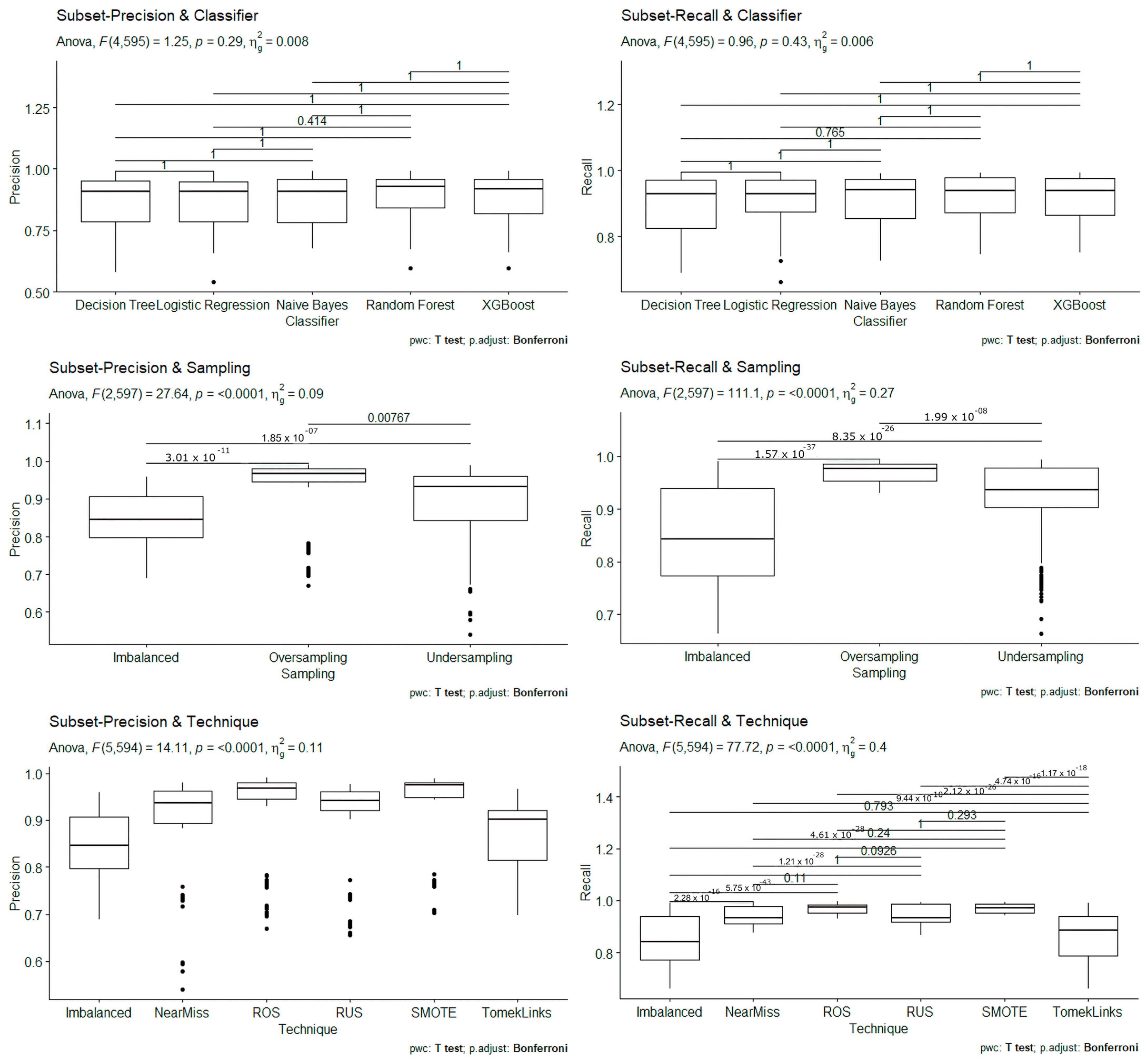
The graph titled ‘Subset—Precision & Classifier’ from Figure 8 shows an F-value of 1.25, and a p-value of 0.29 shows similar scores regardless of the classifier, specifying that all classifiers from subset data are insignificant. There is barely any variation. All the classifiers only perform similarly better than each other.

The graph titled ‘Subset—Recall & Classifier’ has an F-value of 0.96 and a p-value of 0.43, showing that all comparisons from classifiers from subset data for recall are insignificant, worse than precision for the same case. There is variation, but it is closely non-existent. All classifiers have similar scores for recall and precision.

The graph titled ‘Subset—Precision & Sampling shows that all sampling methods with precision scores have shown to be significant, with an F-value of 27.64, and all comparisons are less than the p-value of 0.0001. Oversampling offers the best performance among all the sampling methods, while Imbalanced and Undersampling perform similarly. There is a noticeable difference in scores among all the sampling methods.

The graph titled ‘Subset—Recall & Sampling’ shows that all sampling methods with recall scores have shown to be significant, with an F-value of 111.1, and all comparisons have a p-value of less than 0.0001. However, the recall scores have a more noticeable difference than the precision scores.

The graph titled ‘Subset—Precision & Technique’, for the sampling techniques, an F-value of 14.11 and a p-value less than 0.0001 show slight performance variation from all sampling techniques and Imbalanced data. Imbalanced data is significant compared to other techniques. Imbalanced data has a difference in scores compared to NearMiss, ROS, RUS, and SMOTE. The four sampling techniques have similar scores to TomekLinks and Imbalanced data. This similarity shows that four sampling techniques (NearMiss, ROS, RUS, and SMOTE) can address the imbalanced dataset problem.

The graph titled ‘Subset—Recall & Technique’ shows an F-value of 77.72 and a p-value less than 0.0001 for the sampling techniques. The Imbalanced label (being imbalanced data) and TomekLinks perform similarly to the other sampling techniques (NearMiss, ROS, RUS, and SMOTE).

The ROC Curves in Figure 9 are the highest and lowest performances possible for Subset data. The performance is closely similar for all classifiers from Iterations 5 and 10. Iteration 10 shows a slight decrease in performance from Iteration 5. The highest performance was from Iteration 5 of Random Oversampling. Iteration 10 of NearMiss records the lowest performance found in Iteration 10. Random Forest and XGBoost classifiers have the highest performance, averaging 0.99, and Naive Bayes has the most inferior performance of all classifiers.

Figure 10 presents precision and recall scores for different facets, comparing each sampling technique for subset data. Based on these facets, ROS, RUS, SMOTE, and NearMiss have data points in similar locations compared to the Imbalanced data and TomekLinks technique. By visualizing the different facets, it becomes clear that these four imbalanced sampling techniques were more effective in addressing our class’s imbalanced problem than other techniques.

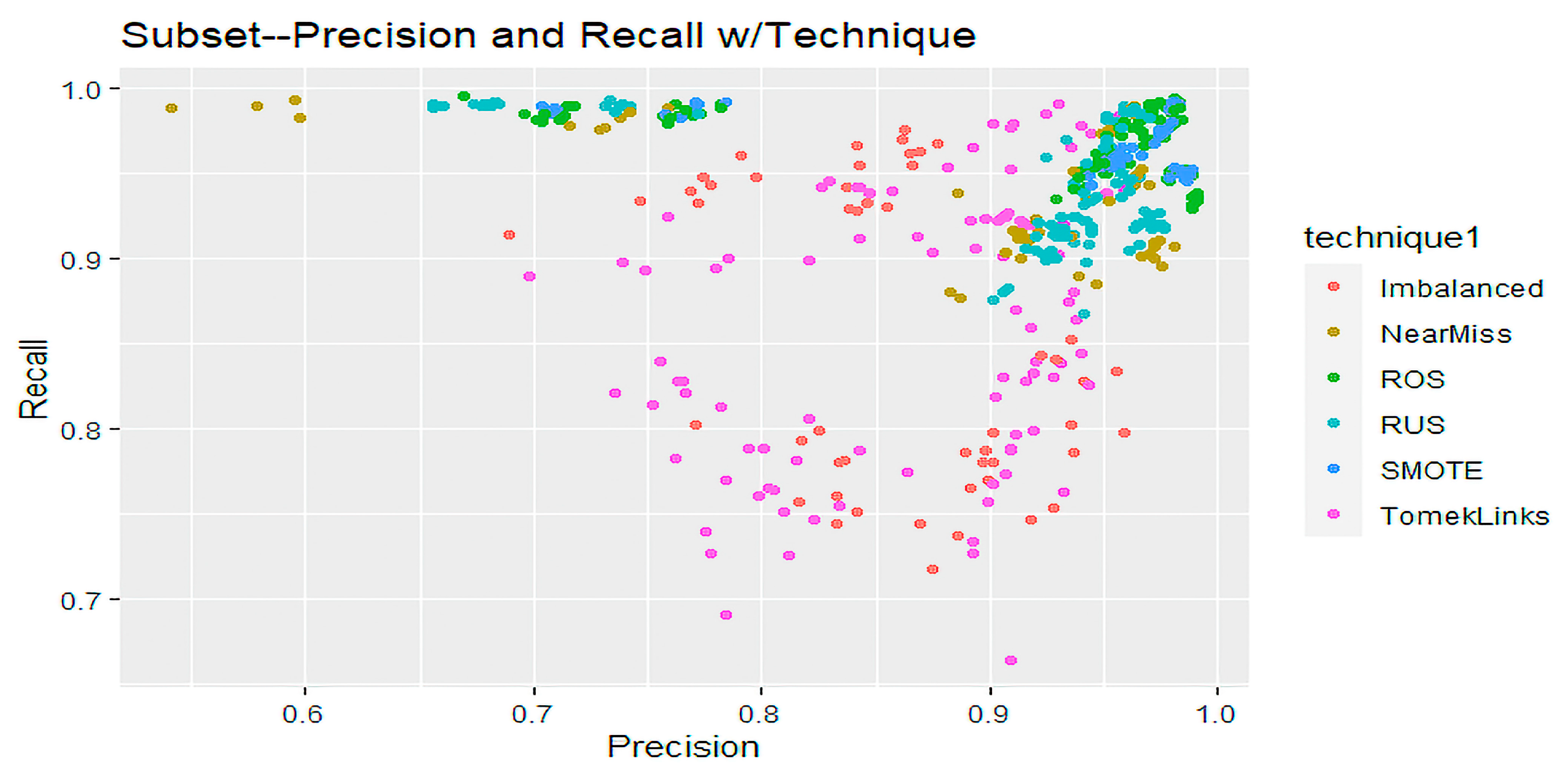
Figure 11 shows a scatter plot of precision and recall in a two-dimensional graph that compares imbalanced sampling techniques for Subset data. Fewer observations from the Subset data supply fewer plots from the MEDFULL data. TomekLinks and Imbalanced have similar patterns where precision and recall are between 69% to 98%. ROS and SMOTE show identical ways of having high recall and precision compared to other techniques, including Imbalanced data.

Figure 12 shows a heatmap of precision and recall in a two-dimensional graph for Subset data. There is a low amount of variability due to the number of observations. The lighter the color, the higher the number of values occupying a particular graph area. The highest scores for precision and recall are easier to find based on the heatmap.

4.3. Model Execution

The four Scikit-learn modules and the XGBoost library assist in executing the five classifiers. The machine learning models use no additional parameters to run the Decision Tree, XGBoost, and Nave Bayes classifiers. Multinomial Naive Bayes is the specific type of Nave Bayes classifier used. The Logistic Regression classifier runs with the following parameters: an l2 penalty, a random state of zero, the lbfgs solver, automatic multi-class, and a maximum of 500 iterations. The Random Forest Classifier runs with the following settings: 1000 estimators and a random state of zero.

To run the experiments, we used multiple workstations in a lab, each with at least 16 GB to 32 GB of RAM. The lab environment has central processing units from 2.5 gigahertz to 5 GHz. Depending on the RAM, each computer runs three to six machine-learning models simultaneously.

However, a Linux cluster with 200 to 800 gigabytes of random-access memory is the recommended environment for executing machine-learning models efficiently. This cluster should be capable of running up to 75 models concurrently in a Unix terminal.

5. Conclusions and Discussion

This work presents robust statistical and exploratory analysis to demonstrate the effects of the performance of ML classifiers and sampling techniques in document datasets; when training on the Subset data, classifiers without sampling techniques achieved an average accuracy of 84.945% and recall of 85.076%. Classifiers trained with sampling techniques achieved an average precision of 90.002% and recall of 93.335%. Without sampling techniques, classifiers on the MEDFULL data achieved an average precision of 73.296% and a recall of 69.636%. Classifiers using sampling techniques achieved an average precision of 71.954% and a recall of 68.706%. The manual document classification approach for MEDFULL data collection has shown not to have a class imbalance issue, and the automatic document classification approach for Subset Data collection has a class imbalance issue. There are fewer observations, patterns, trends, and anomalies in the Subset data. However, it has more variation or effectiveness in performance as measured by ANOVA scores compared to the MEDFULL data while doing exploratory data analysis.

Studies have shown that imbalanced classifiers could perform better on unstructured text data. However, using imbalanced sampling techniques can address the imbalanced dataset problem. However, varying the training, testing sizes, and subsampling data can unpredictably change the performance metrics. In addition, automatic and manual document classification and feature engineering methods can create unexpected results for performance metrics. By using training size variation and subsampling, this paper intends to address the shortcomings of machine learning classification from previous literature regarding performance metrics and exploratory data analysis.

Our future work involves using Deep Learning (DL) algorithms with language models with Bidirectional Encoder Representations from Transformers (BERT) and PyTorch. Adjustments are necessary for finetuning these models and require using a larger dataset that will provide more data to train with to get superior performance from deep learning algorithms. When executing the deep learning models, a researcher can apply similar subsampling, training size variation methods, and other feature engineering techniques. Also, a researcher can use statistical analysis to evaluate the performance of the different deep learning algorithms.