Social Intelligence Mining: Unlocking Insights from X

Abstract

Social trend mining, situated at the confluence of data science and social research, provides a novel lens through which to examine societal dynamics and emerging trends. This paper explores the intricate landscape of social trend mining, with a specific emphasis on discerning leading and lagging trends. Within this context, our study employs social trend mining techniques to scrutinize X (formerly Twitter) data pertaining to risk management, earthquakes, and disasters. A comprehensive comprehension of how individuals perceive the significance of these pivotal facets within disaster risk management is essential for shaping policies that garner public acceptance. This paper sheds light on the intricacies of public sentiment and provides valuable insights for policymakers and researchers alike.

1. Introduction

By harnessing the power of open-access data found on social media platforms and employing advanced analytical techniques, researchers can uncover valuable information about public sentiment and behavior across a range of topics that capture public attention [1,2,3,4,5,6].

The identification of leading and lagging trends is vital for comprehending the temporal dynamics of social phenomena. Analyzing time series data derived from social media platforms and search engines enables the detection of patterns that indicate which trends are leading or lagging [7]. This knowledge can facilitate proactive decision-making, policy formulation, and strategic planning in various domains [8].

In the age of data abundance, Social Intelligence Mining emerges as the key to unlocking a profound understanding of user behavior, preferences, and sentiments [9]. Harnessing the vast sea of online data, including insights from X (formerly twitter), businesses gain a real-time pulse on market dynamics, consumer trends, and competitive intelligence [10]. Moreover, the data hold immense potential for research in the public interest [11].

For instance, extracting pattern from X offers a dynamic lens to scrutinize the popularity of keywords and phrases. They serve myriad purposes, from analyzing public opinion and tracking information propagation to unraveling shifts in consumer behavior. Examples abound of how these data sources have been harnessed for diverse insights (see, for instance [12,13,14,15,16,17,18,19,20,21]).

The landscape of online networks has undergone a seismic shift, largely due to the advent of social media platforms [22]. These platforms, characterized by their openness, interactivity, flexibility, robustness, and creativity, have redefined the way we connect and share [23]. They’ve forged virtual links that mirror real-life social networks, a testament to their small-world charm [24].

As of the beginning of Q3 2023, a staggering 5.19 billion individuals were actively using the internet worldwide. This remarkable trend of internet usage is also on a continuous upward trajectory. Recent data reveal that the world’s online community expanded by over 100 million users in the 12-month period leading up to July 2023 [25].

X, as a prominent social media platform, plays a vital role in today’s digital landscape by providing a space where people can freely share information, express their opinions on events, policies, and other topics, thereby shaping public discourse and influencing societal trends. While X offers a vast trove of information, analyzing it effectively requires the creation of trends through time series analysis [26,27,28,29,30]. This is the core challenge we address in our research. Additionally, having various time series allows us to not only evaluate patterns but also their interactions and interconnections. The critical questions we aim to answer are: Can we assess dependencies across different frequencies within these time series? If so, are we able to discern which time series leads or lags others in terms of frequency and phase differences? Our research provides comprehensive answers to these pivotal questions.

Furthermore, our analysis extends to extracting insights from a network of keywords. This complements our lead and lag analysis, enhancing our understanding of the relationships and dynamics within the data.

The next section unveils our methodology, comprised of various sub-sections, focusing on the mathematical underpinnings of sentiment analysis and network analysis, as well as lead and lag analysis using wavelet transforms.

In the subsection on Sentiment Analysis, we delve into the mathematical formulation of sentiment analysis as a classification problem. This involves mapping textual data to sentiment scores, employing techniques such as the bag-of-words model and sentiment scoring. The classification process is based on thresholding sentiment scores, and supervised learning is used for training the models.

The Network Analysis subsection elucidates the methodology for analyzing complex systems through graphs. This encompasses the representation of networks through adjacency matrices, examining node degrees, and calculating path lengths and centrality measures. Crucial concepts like clustering coefficients and modularity, vital for understanding network structure and community dynamics, are also covered.

In the section on Lead and Lag Analysis, we introduce a novel approach using wavelet transforms to simplify complex time series data and reveal underlying periodic behaviors. This includes both univariate and bivariate cases, exploring how wavelet coherence can uncover relationships between different time series. The application of this methodology to social phenomena is highlighted, showcasing its potential to uncover cyclical patterns in social interest and activities.

Together, these methodologies provide a robust framework for analyzing and interpreting complex data sets, offering insights into sentiment trends, network dynamics, and cyclical patterns in social phenomena.

2. Methodology

2.1. Sentiment Analysis: A Brief Mathematical Perspective

Sentiment analysis, often referred to as opinion mining, entails extracting and understanding sentiments from textual data. In mathematical terms, sentiment analysis can be considered as a classification problem, where a given piece of text t is mapped to a sentiment s. This sentiment could be binary, such as positive or negative, or could span multiple classes, such as positive, negative, neutral, and so on (see, for instance, Refs. [31,32,33]).

2.1.1. Representation of Text

To conduct sentiment analysis mathematically, text first needs to be converted into a format that algorithms can understand. One common representation is the bag-of-words model.

Let D be a dataset containing N textual documents. If V represents the vocabulary of unique words extracted from D, then any text t can be represented as:

$$t=[w_1,w_2,\dots ,w_m]$$

where $w_i$ is the weight (often term frequency) of word i in the text and $m=\left|V\right|$.

2.1.2. Sentiment Scoring

Given a piece of text t, a sentiment score $S\left(t\right)$ can be computed using:

$$S\left(t\right)=\sum _{i=1}^m{w}_i\times P\left(i\right)$$

where $P\left(i\right)$ is the predefined sentiment polarity of word i. This polarity can be positive, negative, or neutral, often represented as values in the range $[-1,1]$.

2.1.3. Classification

Given the sentiment score $S\left(t\right)$ for a text t, classification can be achieved using a threshold $\theta$:

$$\mathrm{Sentiment}\left(t\right)=\left\{\begin{array}{cc}\mathrm{positive}\hfill & \mathrm{if}S\left(t\right)>\theta \hfill \\ \mathrm{negative}\hfill & \mathrm{if}S\left(t\right)<-\theta \hfill \\ \mathrm{neutral}\hfill & \mathrm{otherwise}\hfill \end{array}\right.$$

2.1.4. Training

For supervised sentiment analysis, a training set T consisting of pairs $(t_i,s_i)$ (where $t_i$ is a piece of text and $s_i$ is its corresponding sentiment) is used to learn the function f such that:

$$s_i\approx f\left(t_i\right)$$

for all i.

An optimization algorithm, such as gradient descent, is used to minimize the difference between the predicted sentiment $f\left(t_i\right)$ and the actual sentiment $s_i$.

This subsection provided a succinct mathematical overview of sentiment analysis. In practice, various sophisticated models like neural networks and deep learning architectures can further enhance the accuracy and depth of sentiment analysis.

Sentiment analysis is a complex field that faces numerous challenges, particularly in the area of weighting. Assigning appropriate importance to words or phrases can be intricate due to the nuances and subtleties of human language. Content analysis further complicates the task, as the meaning of words can vary greatly depending on their context, making it difficult to consistently interpret sentiment across diverse content types. Emojis introduce an additional layer of complexity to sentiment analysis, as their meanings are often subjective and culturally varied. In voice analysis, capturing and interpreting nuances like tone and intonation accurately can be challenging, as these aspects significantly influence the conveyed sentiment. Picture analysis involves comprehending visual cues and context, where images can convey intricate emotions and messages that are open to various interpretations. These challenges are amplified when analyzing ’X’ data, which may incorporate a mix of text, emojis, voice, and images. Each of these modalities presents unique interpretation challenges, necessitating sophisticated analysis techniques and a profound understanding of various communication modes.

2.2. Network Analysis

Network analysis is a method used to study the relationships and patterns within interconnected nodes and links in a network. It provides insights into the structure, dynamics, and functions of complex systems, ranging from social networks to transportation systems. The technique is invaluable for identifying influential nodes, clusters, and potential vulnerabilities within a network [34,35,36].

2.2.1. Graph Definition

A graph G is defined as $G=(V,E)$ where:

• V is a set of nodes (vertices). The total number of nodes is denoted as n where $n=\left|V\right|$.
• E is a set of edges (links). The total number of edges is denoted as m where $m=\left|E\right|$.

2.2.2. Adjacency Matrix

The connectivity of nodes in G can be represented by an adjacency matrix, A, of size $n\times n$. If there is an edge between node i and node j, then $A_{ij}=1$; otherwise $A_{ij}=0$.

2.2.3. Degree of a Node

The degree, $d\left(v\right)$, of a node v is the number of edges connected to it. For undirected graphs:

$$d\left(v\right)=\sum _{i=1}^n{A}_{vi}$$

For directed graphs, we can define:

• In-degree, $d_{\mathrm{in}}\left(v\right)$ as the number of edges coming into v.
• Out-degree, $d_{\mathrm{out}}\left(v\right)$ as the number of edges going out of v.

2.2.4. Path and Distance

A path in G is a sequence of nodes such that any two consecutive nodes in the sequence are adjacent. The distance, $d(v_i,v_j)$, between two nodes $v_i$ and $v_j$ is the length (number of edges) of the shortest path connecting them.

2.2.5. Centrality Measures

• Degree Centrality: $C_D\left(v\right)=\frac{d\left(v\right)}{n-1}$
• Betweenness Centrality:

$$C_B\left(v\right)=\sum _{s\ne v\ne t}\frac{{\sigma }_{st}\left(v\right)}{{\sigma }_{st}}$$

where ${\sigma }_{st}$ is the number of shortest paths from s to t, and ${\sigma }_{st}\left(v\right)$ is the number of shortest paths from s to t that pass through v.

2.2.6. Clustering Coefficient

For a node v, it is the ratio of the number of edges between the neighbors of v to the maximum possible number of edges between them. Mathematically:

$$C\left(v\right)=\frac{2e_v}{d\left(v\right)\left(d\right(v)-1)}$$

where $e_v$ is the number of edges between the neighbors of v.

2.2.7. Modularity

Used for community detection in networks. It measures the strength of division of a network into modules. Higher values indicate a strong community structure.

2.3. Lead and Lag Analysis

A wavelet transform is used to transform time series with complex periodic behaviour, to simplified signals, each of which has simple periodic behaviour (with a single period). From a mathematical point of view, a wavelet transform is a generalization of Fourier transform. A Continuous Wavelet Transform, CWT, uses a mother wavelet function $\psi (·)$, to transform a discrete-time time series ${\left\{y_t\right\}}_1^n$, to wavelet coefficients $W_{\psi }\left\{y\right\}(\tau ,s)$, for the time localizing parameter $\tau$ and the scale parameter s.

2.3.1. Univariate Case

The wavelet coefficients $W_{\psi }\left\{y\right\}(\tau ,s)$ are defined as a convolution of time series ${\left\{y_t\right\}}_1^n$ with the localized mother wavelet $\psi (·)$ (named child wavelet), localized in time and frequency space by $\tau$ and s [37]:

$$\begin{array}{c}\hfill W_{\psi }\left\{y\right\}(\tau ,s)=\sum _{t=1}^n{y}_t\frac{1}{\sqrt{s}}\overline{\psi }\left(\frac{t-\tau }{s}\right),\end{array}$$

where $\overline{\psi }(·)$ is the complex conjugate of the mother wavelet $\psi (·)$. The localization parameter $\tau$ exhibits periodic behavior over time, while the scale parameter s localizes the periodic behavior in the frequency domain. Larger values of scale parameter, s, indicates long-term periodic behavior with low frequency. On the other hand, smaller values of the scale parameter s reveal details in short-term periodic patterns with higher frequencies. One commonly used choice for the mother wavelet is the Morlet wavelet [38], which is formulated as follows:

$$\begin{array}{c}\hfill \psi \left(t\right)=c_{\omega }{\pi }^{-\frac{1}{4}}\exp \left\{-\frac{t^2}{2}\right\}\left(e^{i\omega t}-{\kappa }_{\omega }\right),\end{array}$$

where $\omega$ is the angular frequency, and ${\kappa }_{\omega }$ and $c_{\omega }$ are constants defined as:

$$\begin{array}{c}\hfill c_{\omega }={\left(1+e^{-{\omega }^2}-2{\mathrm{e}}^{-\frac{3}{4}{\omega }^2}\right)}^{-\frac{1}{2}},{\kappa }_{\omega }={\mathrm{e}}^{-\frac{1}{2}{\omega }^2}.\end{array}$$

The $\omega =6$ is a proper choice for the angular frequency, since it makes the Morlet wavelet approximately analytic [37]. Large absolute values of $W_{\psi }\left\{y\right\}(\tau ,s)$ indicate powerful periodic pattern in time $\tau$ and period s. The wavelet coefficients can be used to construct the wavelet power spectrum of time series ${\left\{y_t\right\}}_1^n$:

$$\begin{array}{c}\hfill Powe{r}_{\psi }\left\{y\right\}(\tau ,s)=\frac{1}{s}{\left|W_{\psi }\left\{y\right\}(\tau ,s)\right|}^2.\end{array}$$

The wavelet power spectrum, denoted as, $Powe{r}_{\psi }\left\{y\right\}$, is a valuable tool for mapping periodic patterns in a given time series over time. To assess the significance of the wavelet power spectrum, it can be compared against the white noise spectrum using either the asymptotic chi-square statistic [39] or Monte Carlo simulation [40]. The Monte Carlo simulation approach is employed for evaluating the significance of the wavelet power spectrum.

2.3.2. Bivariate Case

Let us now consider time series ${\left\{x_t\right\}}_1^n$ and ${\left\{y_t\right\}}_1^n$ as the bivariate case. A cross wavelet transform can be used to investigate the relation between ${\left\{x_t\right\}}_1^n$ and ${\left\{y_t\right\}}_1^n$ [37]:

$$\begin{array}{c}\hfill W_{\psi }\left\{xy\right\}(\tau ,s)=\frac{1}{s}{W}_{\psi }\left\{x\right\}(\tau ,s){\overline{W}}_{\psi }\left\{y\right\}(\tau ,s),\end{array}$$

where $\overline{W}$ denotes a complex conjugate and $W_{\psi }\left\{x\right\}(\tau ,s)$ and $W_{\psi }\left\{y\right\}(\tau ,s)$ are the wavelet coefficients in CWT of ${\left\{x_t\right\}}_1^n$ and ${\left\{y_t\right\}}_1^n$, respectively. The wavelet cross power spectrum, as modulus of wavelet coefficients, can be used to map the similarities between two time series’ periodic behaviour:

$$\begin{array}{c}\hfill Powe{r}_{\psi }\left\{xy\right\}(\tau ,s)=\left|W_{\psi }\left\{xy\right\}(\tau ,s)\right|.\end{array}$$

The ${Power}_{\psi }\left\{xy\right\}(\tau ,s)$, like covariance, depends on the underlying time series’ unit of measurement and may not properly interpret the degree of association between two series. Wavelet Coherence between two time series ${\left\{x_t\right\}}_1^n$ and ${\left\{y_t\right\}}_1^n$ is defined as the local cross-correlation between the series, localized at time $\tau$ and scale s:

$$\begin{array}{c}\hfill W_{\psi }\left\{xy\right\}(\tau ,s)=\frac{{\left|s{W}_{\psi }\left\{xy\right\}(\tau ,s)\right|}^2}{sPowe{r}_{\psi }\left\{x\right\}(\tau ,s)·sPowe{r}_{\psi }\left\{y\right\}(\tau ,s)},\end{array}$$

where prefix s behind $W_{\psi }$ and ${Power}_{\psi }$ indicates smoothing is required. Similar to the power spectrum, the wavelet coherence between two series can also be examined using Monte Carlo simulation [41,42]. Monte Carlo simulation provides a robust approach for testing the significance of wavelet coherence and assessing the presence of coherent relationships between the two series under investigation.

The continuous wavelet transform (CWT) reveals localized periodic patterns in a given time series ${\left\{y_t\right\}}_1^n$. The wavelet phase indicates the local displacement of the periodic behavior relative to the localization parameter $\tau$, which is shifted across the time domain when $\tau$ is set as the origin. The wavelet phase is typically represented as an angle within the interval [−$\pi$, $\pi$]:

$$\begin{array}{c}\hfill {\Phi }_{\psi }\left\{y\right\}(\tau ,s)={\tan }^{-1}\left(\frac{\mathrm{Im}\left(W_{\psi }\left\{y\right\}(\tau ,s)\right)}{\mathrm{Re}\left(W_{\psi }\left\{y\right\}(\tau ,s)\right)}\right),\end{array}$$

where $\mathrm{Im}(·)$ and $\mathrm{Re}(·)$ are imaginary and Real parts of wavelet coefficient $W_{\psi }\left\{y\right\}\left(\tau ,s\right)$.

Using the cross-wavelet coefficients, one can calculate the difference between wavelet phase from two time series:

$$\begin{array}{c}\hfill {\Phi }_{\psi }^{dif}\left\{xy\right\}(\tau ,s)={\tan }^{-1}\left(\frac{\mathrm{Im}\left(W_{\psi }\left\{xy\right\}(\tau ,s)\right)}{\mathrm{Re}\left(W_{\psi }\left\{xy\right\}(\tau ,s)\right)}\right),\end{array}$$

where ${\Phi }_{\psi }^{dif}\left\{xy\right\}(\tau ,s)$ represents the angular phase difference between two time series ${\left\{x_t\right\}}_1^n$ and ${\left\{y_t\right\}}_1^n$. ${\Phi }_{\psi }^{dif}\left\{xy\right\}(\tau ,s)$ can be used to determine which time series start the periodic pattern first and which one is following, for a given time and frequency interval. Figure 1 shows the simplified interpretation of phase difference between time series ${\left\{x_t\right\}}_1^n$ and ${\left\{y_t\right\}}_1^n$.

Once angular phase difference between two series is in hand, it can be translated to time lag between periodic patterns in two series:

$$\begin{array}{c}\hfill H_{\psi }\left\{xy\right\}(\tau ,s)=\frac{l_s}{2\pi }{\Phi }_{\psi }^{dif}\left\{xy\right\}(\tau ,s),\end{array}$$

where $H_{\psi }\left\{xy\right\}(\tau ,s)$ is temporal phase difference between two series, measured by time unit, $l_s$ is the period length corresponding to scale s and ${\Phi }_{\psi }^{dif}\left\{xy\right\}(\tau ,s)$ is angular phase difference measured in radian.

Various social phenomena can exhibit cyclical patterns [44]. By applying wavelet analysis to the social data, we can uncover the underlying periodic patterns in these phenomena. For example, analyzing people’s interest in a subject through chat discussions or online searches can reveal if there are cycles where this subject becomes popular in society. Similarly, examining the number of participants in a social activity can expose the cycles of outbursts in that particular activity.

3. Results

3.1. Data

A total of 10,053 tweets containing the keyword “Earthquake” were extracted from the X platform (formerly Twitter) between 8:05 AM and 10:30 AM on 9 September 2023, the morning immediately following the Morocco earthquake. Among these, 1060 tweets that were unrelated to the earthquake were filtered out from the dataset. Figure 2 displays word clouds and bar charts showcasing the most frequently used words in the remaining relevant tweets.

In this study, specific search terms and engagement metrics were selected based on their relevance to the research objectives. A careful review of the literature and consultation with domain experts helped identify the key search terms and engagement metrics to be considered. Search terms included relevant keywords and phrases associated with the research topic, ensuring comprehensive coverage of the subject matter. These metrics provided a comprehensive understanding of user behaviour and the level of engagement with the topic of interest. Prior to analysis, the collected data underwent a rigorous cleaning and preprocessing phase to ensure data quality and reliability. This involved removing duplicates, eliminating irrelevant or spam-like content, and addressing any inconsistencies or inaccuracies within the dataset. A newly developed tool was utilized to have a comprehensive overview of gathered data. During the preprocessing stage, data were transformed and structured to facilitate subsequent analysis. Techniques such as text normalization, tokenization, stemming, and removing stop words were employed to standardize the textual data and make them suitable for analysis. Additionally, techniques like data aggregation, segmentation, and filtering were applied to focus on specific subsets of the data or specific time-frames, as relevant to the research objectives. Overall, the methodology employed a combination of data collection, cleaning, and analysis techniques to ensure a robust and systematic approach to examining the internet search and engagement data. This comprehensive methodology facilitated the extraction of valuable insights and trends from the dataset, contributing to a deeper understanding of user behaviour and preferences related to the research topic.

3.2. Sentiment Analysis

Two distinct libraries are utilized for sentiment analysis of extracted tweets. The first library in use is the Microsoft Azure Text Analytics library, while the second library is Sentimentr, which is an advanced version of the “Stanford CoreNLP” library, designed to strike a balance between accuracy and processing speed.

The time series resulting from sentiment analysis is segmented into three distinct components (Figure 3): positive, negative, and neutral, which enhances its informativeness. Additionally, an overall sentiment score is included.

As observed, it is evident that the relative frequency of positive sentiment tweets is notably lower than that of negative sentiment tweets in both sentiment analysis libraries.

The results indicate that both Sentimentr and the Microsoft Azure sentiment libraries demonstrate a greater number of tweets with negative sentiment being posted in a minute compared to those with positive sentiments.

Despite the higher relative frequency of tweets with negative sentiment, the bar charts representing words and key phrases reveal that these negative sentiment tweets predominantly revolve around news-related content and condolences.

3.3. Tweet Trend Index

Here we introduce the Tweet Trend Index (TTI). The Tweet Trend Index is a metric that offers insights into the relative popularity of tweeted terms on X over a specified period of time. It provides data on how often particular keywords or topics have been tweeted over the time and when the interest in tweeting on those keywords is in the peak. The data are typically presented as a relative index, with the highest point of tweeted interest during the specified time frame being assigned a value of 100, and other data points are scaled relative to this peak.

The Tweet Trend Index (TTI) at time t is then calculated as follows:

$$TT{I}_t=\frac{N_t}{max\left(N_t\right)}\times 100,t=1,...,T,$$

where $N_t$ is the number of tweets or mentions related to a specific keyword or topic during time period t (i.e., during tth time interval) and T is the total number of observed time periods.

Figure 4 illustrates TTI for tweets categorized by sentiment, including neutral, positive, and negative sentiments. This graph provides a valuable perspective on how the TTI fluctuates over time, and it is evident that the sentiment peaks vary significantly. Furthermore, this visualization emphasizes that the choice of sentiment analysis tools or methods can lead to variations in the TTI outcomes.

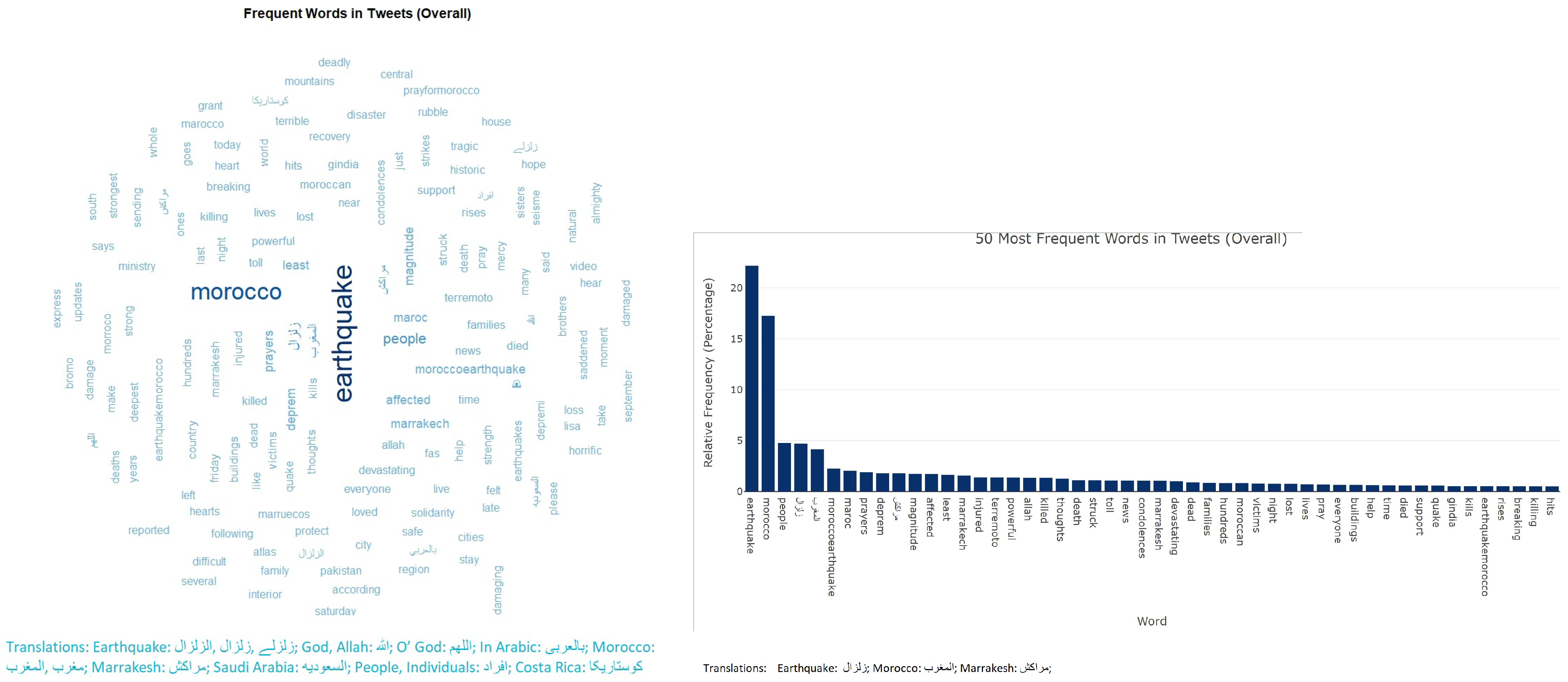
3.4. Coherence Analysis

To explore the connection between periodic patterns in tweets with positive, negative, and neutral sentiments, we applied continuous wavelet transform using the Morlet mother wavelet function. The wavelet power spectrum of the three time series from the Microsoft Azure sentiment library, the first three rows of Figure 5 suggest that the negative sentiment time series exhibits the strongest wavelet power. Moreover, a majority of the significant periodic patterns have periods shorter than 16 min. Interestingly, both the negative and neutral sentiment time series display notable periodic patterns with longer periods.

Conversely, results obtained using the Sentimentr package indicate that the neutral sentiment time series boasts the highest wavelet power. Once again, a significant proportion of these periodic patterns have periods shorter than 16 min. Intriguingly, in the positive and neutral sentiment time series, we observe the presence of substantial periodic patterns with longer periods.

To examine the significant relationships between periodic behaviors in sentiment time series from different sentiment libraries, we computed the wavelet coherence for each pair of sentiment time series.

As illustrated in Figure 5 (the last three rows), for the Microsoft Azure results, the sentiment time series exhibit significant coherence across various periods. However, our focus should be on periods with significant periodic patterns in both series for each sentiment pair.

• In the top panel:

Positive and negative sentiment time series display substantial coherence, particularly in periodic patterns with durations shorter than 16 min. Before 9 AM, the negative sentiment’s periodic pattern predominates, while after 9 AM, the positive sentiment’s periodic pattern takes the lead.

• In the middle panel:

Positive and neutral sentiment time series exhibit significant coherence, primarily in periodic patterns lasting between 4 and 16 min. Notably, most of this coherence occurs after 9 AM. Between 9 and 10 AM, the neutral sentiment time series leads, but after 10 AM, the behavior of cyclical patterns with different period lengths diverges. In patterns with longer periods (lower frequency), the positive sentiment time series leads, while in patterns with shorter periods (higher frequency), the neutral sentiment time series leads. Interestingly, in most periods with significant coherence between positive and neutral sentiment time series, they are out of phase, indicating a negative correlation at those frequencies.

• In the bottom panel:

Negative and neutral sentiment time series demonstrate significant coherence, mainly in periodic patterns lasting between 8 and 16 min, as well as patterns around 32 min. However, significant coherence in longer periods (low-frequency cycles) tends to occur after 9 AM. Before 9 AM, the negative sentiment time series leads in mid-range periodic patterns (periods between 8 and 16 min), while the neutral sentiment time series leads in shorter and longer-range periods. After 9 AM, when coherence between the two series is significant, the neutral sentiment time series predominates.

The same analysis can be interpreted for the Sentimentr library. In the top panel, for instance, the majority of arrows indicate that in cyclical patterns with shorter durations, the positive sentiment time series takes the lead, while in longer periods, the negative sentiment time series leads the way.

The overall findings suggest that all sentiment time series exhibit significant periodic patterns with varying period lengths. In essence, the number of posted tweets with positive, negative, or neutral sentiments follows distinct periodic patterns.

Interestingly, even though the negative sentiment time series consistently has higher values compared to the positive sentiment time series, it does not consistently lead the periodic behavior of the two time series.

It’s noteworthy that the periodic behavior of the three sentiment time series and their interrelation undergo substantial changes over time.

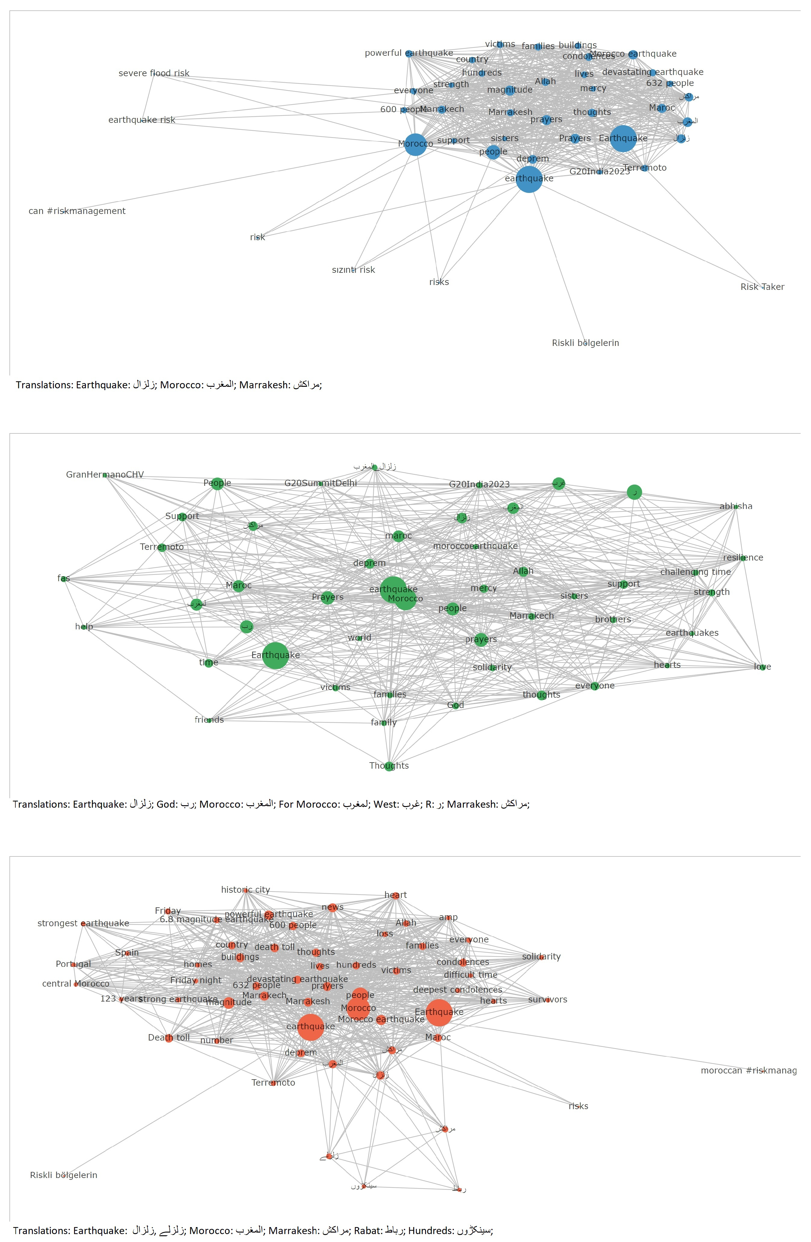
3.5. Network Analysis

In our increasingly interconnected world, network analysis has emerged as a vital tool for uncovering hidden patterns, relationships, and valuable insights. It goes beyond individual entities to explore the intricate web of connections that shape our modern existence.

Figure 6 provides a visual representation of the network analysis conducted on the extracted tweets related to Morocco and earthquake data. In this analysis, we have taken into account tweets categorized as positive, negative, neutral, and overall sentiments to gain a comprehensive understanding of the conversation.

Upon closer examination, several intriguing patterns emerge. Notably, we observe a connection between keywords such as “risk” and “risk management” and the term “earthquake.” This linkage indicates that while citizens express their concerns about earthquakes and their potential impacts, there is also an awareness of the importance of risk management strategies to mitigate these risks effectively.

Additionally, the network analysis allows us to distinguish between positive, negative, and neutral tweets. This differentiation provides valuable insights into the sentiment of the discussions surrounding earthquakes in Morocco. Positive tweets may reflect resilience, preparedness, or hope, while negative ones might signify anxiety, fear, or frustration. The neutral tweets offer a balanced perspective, often containing factual information.

By leveraging network analysis, we can uncover the intricate web of connections between words and sentiments within the Twitter data, shedding light on the multifaceted nature of conversations around earthquakes in Morocco. This deeper understanding of the online discourse can inform disaster management strategies, community engagement efforts, and public awareness campaigns to ensure a more informed and prepared society in the face of seismic events.

4. Discussion

The research leveraging open-access data from social media platforms can substantially benefit a diverse array of groups, including policy makers, businesses, public health officials, academics, NGOs, media, and public relations professionals. For policy makers and governmental organizations, it provides deep insights into public sentiment, aiding in informed decision-making and policy formulation. Businesses and marketers can harness the data to understand consumer behavior and tailor their strategies accordingly. Public health officials can use these insights for effective communication and monitoring of health campaigns, while academics gain valuable data for sociological and psychological research. NGOs can leverage this information to drive social change initiatives and engage communities more effectively. Media and journalists can utilize these insights to track trending topics and create resonant content, while PR professionals can use the data for reputation management and strategic communication. this research offers a comprehensive understanding of societal trends and online behavior, essential for various sectors to respond proactively to public needs and changes in the digital landscape.

When discussing the limitations of various analytical methods, including sentiment analysis, network analysis, and coherence analysis using wavelet transforms, it’s essential to acknowledge their respective constraints to provide a balanced perspective.

4.1. SentimentAnalysis

A notable limitation of sentiment analysis is its reliance on predefined algorithms and lexicons, which may not fully capture the nuances and context of language, leading to potential inaccuracies in interpreting sarcasm, idioms, or culturally specific expressions.

4.2. Network Analysis

Network analysis, while powerful in uncovering relationships and patterns within data, can be constrained by its dependency on the quality and completeness of the underlying data; inaccuracies or missing information can lead to incomplete or skewed understanding of the network dynamics.

4.3. Coherence Analysis Using Wavelet Transforms

Coherence analysis through wavelet transforms, although effective in identifying periodic patterns and correlations in time series data, is limited by its sensitivity to non-stationarities in the data and the subjective nature of choosing appropriate wavelet functions and parameters, which can impact the interpretation of results.

Each of these sentences acknowledges critical aspects where the methods might fall short, emphasizing the need for careful consideration and complementary approaches in data analysis.

Furthermore, combination of sentiment analysis, network analysis, and coherence analysis using wavelet transforms can offer a multi-dimensional approach to disaster risk management, particularly for earthquakes. Each method brings unique insights that, when integrated, provide a comprehensive understanding of public perception, communication patterns, and temporal dynamics related to earthquake risks.

4.4. Sentiment Analysis for Understanding Public Reaction and Awareness

(a)

Sentiment analysis of social media data, especially around the time of an earthquake, can provide real-time insights into public emotions, concerns, and awareness levels.

(b)

Identifying shifts in sentiment (e.g., fear, confusion, or relief) can guide emergency services in tailoring their communication and support strategies to address public concerns effectively.

4.5. Network Analysis for Mapping Communication Patterns

(a)

Network analysis can identify key influencers, communication hubs, and information dissemination patterns within social networks.

(b)

Understanding how information about earthquakes spreads through networks enables authorities to identify misinformation and target outreach efforts more effectively. It also helps in leveraging influential nodes (like popular social media accounts) to disseminate accurate information quickly.

4.6. Coherence Analysis for Temporal Dynamics

(a)

Coherence analysis using wavelet transforms can uncover temporal patterns in public discussions and sentiments about earthquakes.

(b)

This can help predict when public interest or concern might peak, allowing for timely interventions, like public education campaigns or readiness drills.

4.7. Integrated Application in Disaster Risk Management

1.

Pre-Disaster: By analyzing sentiment and network structures, authorities can assess public preparedness and tailor educational campaigns to improve readiness. Coherence analysis can indicate optimal times for releasing information.

2.

During a Disaster: Real-time sentiment analysis can gauge public mood and needs, guiding immediate response strategies. Network analysis can help manage the flow of information, ensuring accurate and efficient communication.

3.

Post-Disaster: Continued analysis aids in monitoring public morale and the spread of information about aftershocks, relief efforts, and recovery resources. It can also help in understanding community resilience and long-term recovery needs.

Combining these methods offers a holistic view of how the public perceives and reacts to earthquake risks and how information circulates before, during, and after an event. This integrated approach can significantly enhance disaster risk management strategies, from preparedness to recovery phases.

5. Conclusions

In the age of information abundance, harnessing the wealth of open-access data from social media platforms is instrumental in deciphering public sentiment and understanding evolving social phenomena. This study delved into the temporal dynamics of social trends, unearthing valuable insights from data derived from X (formerly Twitter). The application of advanced analytical techniques allowed us to reveal significant patterns and trends in online conversations. By dissecting the temporal dynamics of social trends and employing wavelet analysis, we were able to distinguish leading and lagging trends across a variety of sentiment categories. This knowledge is essential for proactive decision-making, policy formulation, and strategic planning in diverse domains.

The results of our analysis revealed that the relative frequency of negative sentiment tweets surpassed that of positive sentiment in both sentiment analysis libraries. These negative sentiments often revolved around news-related content and condolences. This insight offers a nuanced understanding of how users express their emotions and engage with social issues during significant events, such as earthquakes.

Furthermore, our coherence analysis illuminated the relationships between periodic patterns in tweets with positive, negative, and neutral sentiments. These results are essential for understanding how different sentiments interplay in online conversations, offering valuable insights for communication strategies and community engagement during critical events.

Lastly, our network analysis provided a comprehensive view of conversations related to earthquakes in Morocco. Notably, keywords such as “risk” and “risk management” were linked to “earthquake”, emphasizing public awareness of risk mitigation strategies during seismic events. By differentiating between positive, negative, and neutral tweets, we gained a deeper understanding of the emotional spectrum surrounding this topic.

In conclusion, this study demonstrates the power of social media data analysis in uncovering temporal dynamics and user sentiments in online conversations. It provides a foundation for proactive decision-making, informed disaster management, and community engagement efforts during significant events, ultimately contributing to a more resilient and prepared society. The continuous evolution of online networks ensures that social intelligence mining remains a dynamic and valuable field for researchers and organizations alike.

It is crucial to recognize that sentiment analysis libraries may contain inherent biases, and the interpretation of sentiments can often be subjective [45]. The results presented here are based on a specific sample size extracted, and it’s important to note that changing the data, period, or extending the time horizon could alter the outcomes. Therefore, potential biases in sentiment analysis libraries should be carefully considered, as these biases might significantly impact the interpretation of the results.

References

1. Karami, A.; Shah, V.; Mammadov, T. Mining Public Opinion about Economic Issues: Twitter and the U.S. Presidential Election. Int. J. Strateg. Decis. Sci. (IJSDS) 2020, 11, 89–104. [Google Scholar] [CrossRef]
2. Silva, E.S.; Hassani, H.; Madsen, D.Ø.; Gee, L. Googling Fashion: Forecasting Fashion Consumer Behaviour Using Google Trends. Soc. Sci. 2019, 8, 111. [Google Scholar] [CrossRef]
3. Silva, E.S.; Hassani, H.; Madsen, D.Ø. Big Data in fashion: Transforming the retail sector. J. Bus. Strategy 2020, 41, 21–27. [Google Scholar] [CrossRef]
4. Bruns, A.; Stieglitz, S. Towards more systematic Twitter analysis: Metrics for tweeting activities. Int. J. Soc. Res. Methodol. 2013, 16, 91–108. [Google Scholar] [CrossRef]
5. Negrón, J.B. EULAR2018: The Annual European Congress of Rheumatology—A Twitter hashtag analysis. Rheumatol. Int. 2019, 39, 893–899. [Google Scholar] [CrossRef] [PubMed]
6. Thakur, N. Monkey Pox 2022 Tweets: A Large-Scale Twitter Dataset on the 2022 Monkeypox Outbreak, Findings from Analysis of Tweets, and Open Research Questions. Infect. Dis. Rep. 2022, 14, 855–883. [Google Scholar] [CrossRef] [PubMed]
7. Hassani, H.; Komendantova, N.; Rovenskaya, E.; Yeganegi, M.R. Social Trend Mining: Lead or Lag. Big Data Cogn. Comput. 2023, 7, 171. [Google Scholar] [CrossRef]
8. Vosen, S.; Schmidt, T. Forecasting private consumption: Survey-based indicators vs. Google trends. J. Forecast. 2011, 30, 565–578. [Google Scholar] [CrossRef]
9. He, W.; Zha, S.; Li, L. Social media competitive analysis and text mining: A case study in the pizza industry. Int. J. Inf. Manag. 2013, 33, 464–472. [Google Scholar] [CrossRef]
10. Stieglitz, S.; Dang-Xuan, L. Social media and political communication: A social media analytics framework. Soc. Netw. Anal. Min. 2013, 3, 1277–1291. [Google Scholar] [CrossRef]
11. Fan, W.; Gordon, M.D. The power of social media analytics. Commun. ACM 2014, 57, 74–81. [Google Scholar] [CrossRef]
12. Bastos, M.T.; Travitzki, R.; Raimundo, R. Tweeting Political Dissent: Retweets as Pamphlets in #FreeIran, #FreeVenzuela, #Jan25, #SpanishRevolution and #OccupyWallSt, IPP2012; University of Oxford: Oxford, UK, 2012. [Google Scholar]
13. Bastos, M.T.; Travitzki, R.; Puschmann, C. What sticks with whom? Twitter follower- followee networks and news classification. In Proceedings of the 6th International AAAI Conference on Weblogs and Social Media—Workshop on the Potential of Social Media Tools and Data for Journalists in the News Media Industry, Dublin, Ireland, 4–7 June 2012. [Google Scholar]
14. Suh, B.; Hong, L.; Pirolli, P.; Chi, E.H. Want to be Retweeted? Large scale analytics on factors impacting Retweet in Twitter network. In Proceedings of the SOCIALCOM’10 Proceedings of the 2010 IEEE Second International Conference on Social Computing, Minneapolis, MN, USA, 20–22 August 2020; pp. 177–184. [Google Scholar]
15. Go, A.; Bhayani, R.; Huang, L. Twitter Sentiment Classification Using Distant Supervision; Technical Report, Stanford Digital Library Technologies Project; Stanford University: Stanford, CA, USA, 2009. [Google Scholar]
16. Hajibagheri, A.; Sukthankar, G. Political Polarization over Global Warming: Analyzing Twitter Data on Climate Change; Academy of Science and Engineering (ASE): Greensboro, NC, USA, 2014. [Google Scholar]
17. Jahanbakhsh, K.; Moon, Y. The predictive power of social media: On the predictability of U.S presidential elections using twitter. arXiv 2014, arXiv:1407.0622. [Google Scholar]
18. Japkowicz, N.; Shah, K. (Eds.) Evaluating Learning Algorithms: A Classification Perspective, 1st ed.; Cambridge University Press: Cambridge, UK, 2011. [Google Scholar]
19. Johnson, C.; Shukla, P.; Shukla, S. On Classifying the Political Sentiment of Tweets. 2012. Available online: https://www.cs.utexas.edu/ (accessed on 25 October 2023).
20. Kumar, S.; Morstatter, F.; Liu, H. Twitter Data Analytics; Springer: New York, NY, USA, 2014. [Google Scholar]
21. Saif, H.; He, Y.; Alani, H. Semantic sentiment analysis of twitter. In Proceedings of the 11th International Semantic Web Conference—ISWC 2012, Boston, MA, USA, 11–15 November 2012; pp. 508–524. [Google Scholar]
22. Ellison, N.B.; Steinfield, C.; Lampe, C. The benefits of Facebook “friends”: Social capital and college students’ use of online social network sites. J. Comput.-Mediat. Commun. 2007, 12, 1143–1168. [Google Scholar] [CrossRef]
23. Boyd, D.M.; Ellison, N.B. Social network sites: Definition, history, and scholarship. J. Comput.-Mediat. Commun. 2007, 13, 210–230. [Google Scholar] [CrossRef]
24. Haythornthwaite, C. Social networks and Internet connectivity effects. Inf. Commun. Soc. 2005, 8, 125–147. [Google Scholar] [CrossRef]
25. Data Portal. Global Digital Overview. Available online: https://datareportal.com/global-digital-overview (accessed on 23 October 2023).
26. Kumar, S.; Morstatter, F.; Liu, H. Twitter Data Analytics; Springer: Berlin/Heidelberg, Germany, 2014; ISBN 978-1-4614-9372-3. [Google Scholar]
27. Russell, M.A.; Klassen, M. Mining the Social Web: Data Mining Facebook, Twitter, LinkedIn, Instagram, GitHub, and More, 3rd ed.; O’Reilly Media: Sebastopol, CA, USA, 2019; ISBN 978-1491985045. [Google Scholar]
28. Liu, B. Sentiment Analysis and Opinion Mining; Morgan and Claypool Publishers: San Rafael, CA, USA, 2012; ISBN 978-1608458844. [Google Scholar]
29. Golbeck, J. Analyzing the Social Web; Morgan Kaufmann: Burlington, MA, USA, 2013; ISBN 978-0124055315. [Google Scholar]
30. Mejova, Y.; Weber, I.; Macy, M.W. Twitter: A Digital Socioscope; Cambridge University Press: Cambridge, UK, 2015; ISBN 978-1107500076. [Google Scholar]
31. Cambria, E.; White, B. Jumping NLP curves: A review of natural language processing research. IEEE Comput. Intell. Mag. 2020, 9, 48–57. [Google Scholar] [CrossRef]
32. Zhang, L.; Wang, S.; Liu, B. Deep learning for sentiment analysis: A survey. Wiley Interdiscip. Rev. Data Min. Knowl. Discov. 2018, 8, e1253. [Google Scholar] [CrossRef]
33. Giachanou, A.; Crestani, F. Like it or not: A survey of Twitter sentiment analysis methods. ACM Comput. Surv. (CSUR) 2016, 49, 1–41. [Google Scholar] [CrossRef]
34. Lu, L.; Chen, D.; Ren, X.-L.; Zhang, Q.-M.; Zhang, Y.-C.; Zhou, T. Vital nodes identification in complex networks. Phys. Rep. 2016, 650, 1–63. [Google Scholar] [CrossRef]
35. Barabási, A.-L.; Pósfai, M. Network Science; Cambridge University Press: Cambridge, UK, 2016. [Google Scholar]
36. Boccaletti, S.; Bianconi, G.; Criado, R.; Del Genio, C.I.; Gómez-Gardeñes, J.; Romance, M.; Sendiña-Nadal, I.; Wang, Z.; Zanin, M. The Structure and Dynamics of Multilayer Networks. Phys. Rep. 2014, 544, 1–122. [Google Scholar] [CrossRef]
37. Carmona, R.; Hwang, W.L.; Torresani, B. Practical Time Frequency Analysis: Gabor and Wavelet Transforms with an Implementation in S; Academic Press: San Diego, CA, USA, 1998. [Google Scholar]
38. Morlet, J.; Arens, G.; Fourgeau, E.; Giard, D. Wave propagation and sampling theory—Part I: Complex signal and scattering in multilayered media. Geophysics 1982, 47, 203–221. [Google Scholar] [CrossRef]
39. Torrence, C.; Compo, G.P. A practical guide to wavelet analysis. Bull. Am. Meteorol. Soc. 1998, 79, 61–78. [Google Scholar] [CrossRef]
40. Ge, Z. Significance tests for the wavelet power and the wavelet power spectrum. Ann. Geophys 2007, 25, 2259–2269. [Google Scholar] [CrossRef]
41. Maraun, D.; Kurths, J. Cross wavelet analysis: Significance testing and pitfalls. Nonlinear Process. Geophys. 2004, 11, 505–514. [Google Scholar] [CrossRef]
42. Ge, Z. Significance tests for the wavelet cross spectrum and wavelet linear coherence. Ann. Geophys 2008, 26, 3819–3829. [Google Scholar] [CrossRef]
43. Rósch, A.; Schmidbauer, H. WaveletComp 1.1: A Guided Tour through the R Package. 2018. Available online: http://www.hsstat.com/projects/WaveletComp/WaveletComp_guided_tour.pdf (accessed on 23 October 2023).
44. Berestycki, H.; Rossi, L.; Rodríguez, N. Periodic cycles of social outbursts of activity. J. Differ. Equ. 2018, 264, 163–196. [Google Scholar] [CrossRef]
45. Petz, G.; Karpowicz, M.; Fürschuß, H.; Auinger, A.; Stříteský, V.; Holzinger, A. Computational approaches for mining user’s opinions on the Web 2.0. Inf. Process. Manag. 2014, 50, 899–908. [Google Scholar] [CrossRef]
Figure 1. Phase difference interpretation for signals x and y [43].
Make 05 00093 g001
Figure 2. The Word Cloud and the Most Frequent Words from Key Phrases in Extracted Tweets.
Make 05 00093 g002
Figure 3. The overall sentiment of tweets categorized as neutral, positive, and negative and Frequent words in negative sentiment tweets.
Make 05 00093 g003
Figure 4. The overall Index of tweets’ sentiment categorized as neutral, positive, and negative.
Make 05 00093 g004
Figure 5. Lag and Lead Sentiment Analysis for Extracted Tweets.
Make 05 00093 g005
Figure 6. Network Analysis of Moroccan Earthquake Tweets: Insights into Sentiment and Risk Management.
Make 05 00093 g006
Disclaimer/Publisher’s Note: The statements, opinions and data contained in all publications are solely those of the individual author(s) and contributor(s) and not of MDPI and/or the editor(s). MDPI and/or the editor(s) disclaim responsibility for any injury to people or property resulting from any ideas, methods, instructions or products referred to in the content.