Article

PCa-Clf: A Classifier of Prostate Cancer Patients into Patients with Indolent and Aggressive Tumors Using Machine Learning

by
Yashwanth Karthik Kumar Mamidi
1,
Tarun Karthik Kumar Mamidi
2,3,
Md Wasi Ul Kabir
1,
Jiande Wu
4,
Md Tamjidul Hoque
1,* and
Chindo Hicks
4,*
1
Department of Computer Science, University of New Orleans, New Orleans, LA 70148, USA
2
Department of Genetics, Heersink School of Medicine, The University of Alabama at Birmingham, 720 20th Street S, Birmingham, AL 35294, USA
3
Center for Computational Genomics and Data Science, The University of Alabama at Birmingham, 912 18th Street S, Birmingham, AL 35233, USA
4
Department of Genetics and the Bioinformatics and Genomics Program, Louisiana State University Health Sciences Center, School of Medicine, 533 Bolivar Street, New Orleans, LA 70112, USA
*
Authors to whom correspondence should be addressed.
Mach. Learn. Knowl. Extr. 2023, 5(4), 1302-1319; https://doi.org/10.3390/make5040066
Submission received: 5 July 2023 / Revised: 20 September 2023 / Accepted: 25 September 2023 / Published: 27 September 2023
(This article belongs to the Special Issue Machine Learning for Biomedical Data Processing)

Abstract

:
A critical unmet medical need in prostate cancer (PCa) clinical management centers around distinguishing indolent from aggressive tumors. Traditionally, Gleason grading has been utilized for this purpose. However, tumor classification using Gleason Grade 7 is often ambiguous, as the clinical behavior of these tumors follows a variable clinical course. This study aimed to investigate the application of machine learning techniques (ML) to classify patients into indolent and aggressive PCas. We used gene expression data from The Cancer Genome Atlas and compared gene expression levels between indolent and aggressive tumors to identify features for developing and validating a range of ML and stacking algorithms. ML algorithms accurately distinguished indolent from aggressive PCas. With the accuracy of 96%, the stacking model was superior to individual ML algorithms when all samples with primary Gleason Grades 6 to 10 were used. Excluding samples with Gleason Grade 7 improved accuracy to 97%. This study shows that ML algorithms and stacking models are powerful approaches for the accurate classification of indolent versus aggressive PCas. Future implementation of this methodology may significantly impact clinical decision making and patient outcomes in the clinical management of prostate cancer.

1. Introduction

Prostate cancer (PCa) is the most common solid tumor and the second most common cause of cancer death in men in the United States [1]. Treatment decisions for PCa patients are guided by various risk stratification algorithms [2]. These stratification algorithms identify and predict patients at high risk of developing aggressive diseases [2]. Among the parameters used, the most potent predictor of PCa mortality is Gleason Grade (GG) scoring, which ranges from 6 to 10 [3,4]. The majority of PCas are indolent, presenting GG 6 [3,4]. These cancers are associated with very low cancer-specific mortality rates, even without therapy [3]. Localized high-grade PCas with lethal potential present GGs 8 to 10 [3,4]. These tumors are aggressive, progress rapidly to metastatic disease, and are often lethal [3,4]. Intermediate-grade PCas present GG 7. These cancers present a much more variable clinical course, with some behaving like GG 6 and others behaving like GGs 8–10 [3,4]. Although current stratification protocols such as GG scoring are moderately effective, significant challenges remain in classifying PCas into indolent versus aggressive tumors. Thus, a critical unmet medical need in the clinical management of PCa is the lack of algorithms to accurately distinguish indolent from aggressive tumors. There is an urgent need to develop algorithms that can accurately distinguish indolent tumors from aggressive tumors, which could be prioritized for treatment.
PCa screening using prostate-specific antigen (PSA) has led to earlier detection of PCa, with fewer men today being diagnosed with metastatic disease [5]. However, although PSA has reduced the mortality rate, it has also resulted in unintended consequences. The unintended consequences include over-diagnosis, which leads to the over-treatment of patients with indolent PCa, and the under-treatment of patients with aggressive disease with lethal potential. Concerns about PSA-based screening led to the US Preventive Services Task Force issuing a D-grade recommendation for its use in 2012 [6]. Importantly, a US Preventive Services Task Force review concluded that PSA-based screening results in either a small or no reduction in prostate cancer-specific mortality [7]. PSA screening is also associated with harms related to subsequent treatments and evaluation—some of which may be unnecessary. These concerns have heightened the need to develop novel risk stratification algorithms to identify patients at high risk of developing aggressive tumors, who could be prioritized for treatment, and the discovery of molecular markers separating indolent tumors from tumors with lethal potential.
Recently, there has been growing interest in the use of machine learning algorithms for risk stratification in PCa and other cancer patients [8,9,10]. Lei Yang et al. [8] used random walk with restart algorithm (RWRA) and graph-regularized non-negative matrix factorization (GNMF) methods for the molecular classification of PCa. They integrated somatic mutation profiles and molecular networks using data from The Cancer Genome Atlas (TCGA), achieving the accuracy of 82.54% [8]. Using RNA-Seq data from TCGA on breast cancer, Danaee et al. [9] applied deep learning stacking algorithms for the discovery of potential clinically actionable biomarkers in breast cancer. These investigators also explored the potential use of different ML methods, including artificial neural network (ANN), Support Vector Machine (SVM), SVM with linear kernel (SVM-LK), and SVM with radial basis function kernel (SVM-RBF) [9]. Takeuchi et al. [10] implemented deep learning with a multilayer artificial neural network (ANN) to predict PCa. They found that improvements needed to be made before the algorithms could be considered suitable for clinical applications [10]. Wulczyn et al. [11] designed an AI-based system to forecast mortality specific to prostate cancer using Gleason grading. They later assessed this system’s efficacy in categorizing risk using a separate retrospective study of 2807 prostatectomy cases. However, algorithms for the accurate classification of PCa patients with indolent versus aggressive PCas to guide clinical decision making are lacking. The development and application of accurate risk classification of PCa patients into those with truly indolent tumors and those with truly aggressive tumors have the promise of improving the clinical management of PCa by eliminating the dilemma faced by clinical oncologists of over-treating individuals with indolent tumors and undertreating individuals diagnosed with aggressive tumors.
To address this critical unmet medical need, we propose using machine learning (ML) models to classify PCa patients into two groups: those with genuinely indolent tumors, which could be safely monitored, versus those with aggressive tumors, which could be prioritized for treatment. The rationale and scientific premise are that implementing ML promises to stratify patients more accurately and thus could guide therapeutic decision making and eliminate the unintended consequences resulting from current protocols. Our working hypothesis posits that genomic alterations in patients diagnosed with indolent and aggressive tumors may result in measurable changes capable of accurately distinguishing indolent tumors from aggressive ones. We addressed this hypothesis using gene expression data linked with clinical information on patients diagnosed with indolent and aggressive PCas from The Cancer Genome Atlas (TCGA). Differential Expression Analysis and Genetic Algorithm techniques were used to identify the number of features/genes associated with the two diseases and to distinguish the two types of PCa used in model development and validation. We then utilized various ML classifiers and 10-fold cross-validation to minimize misclassification rates and enhance accuracy compared with previous research efforts. Additionally, the use of a stacking-based ML approach was investigated, combining different ML classifiers with 10-fold cross-validation to improve model performance. For this study’s purposes, the terms features and genes are used interchangeably throughout the investigation.

2. Experimental Materials and Methods

2.1. Source of Transcriptome and Clinical Datasets

We used publicly available gene expression data linked with clinical information on indolent and aggressive PCas from TCGA generated using RNA sequencing [12]. The dataset was downloaded from the Genomics Data Commons portal using the data transfer tool [13]. Because the same TCGA barcode structure was used for both clinical data and transcriptome data, we used the barcode structure to integrate patient-based clinical data with sample-based genomic data [13]. The original gene expression dataset included N = 547 samples distributed as follows: N = 45 samples as indolent (GG = 6), 246 samples as intermediate (GG = 7), 204 as aggressive with lethal potential (GGs 8–10), and 52 control samples. After annotating gene expression data with clinical information, the American Urological Association classification protocol [14] was used to verify and validate tumor classification according to GG. We used the protocol to assign the tumors to either the indolent or aggressive category, consistently with the guidelines [14]. Because GG7 follows a variable clinical course, the tumor samples from GG7 were either classified as 3 + 4 (primary + secondary) and assigned to GG = 6 as indolent, or as 4 + 3 (primary + secondary) and assigned to GGs = 8–10 as aggressive, consistently with current classification guidelines [14]. The overall project design and execution workflow are shown in Figure 1. This visual representation provides an overview of the key steps and processes involved in the project’s methodology and execution.

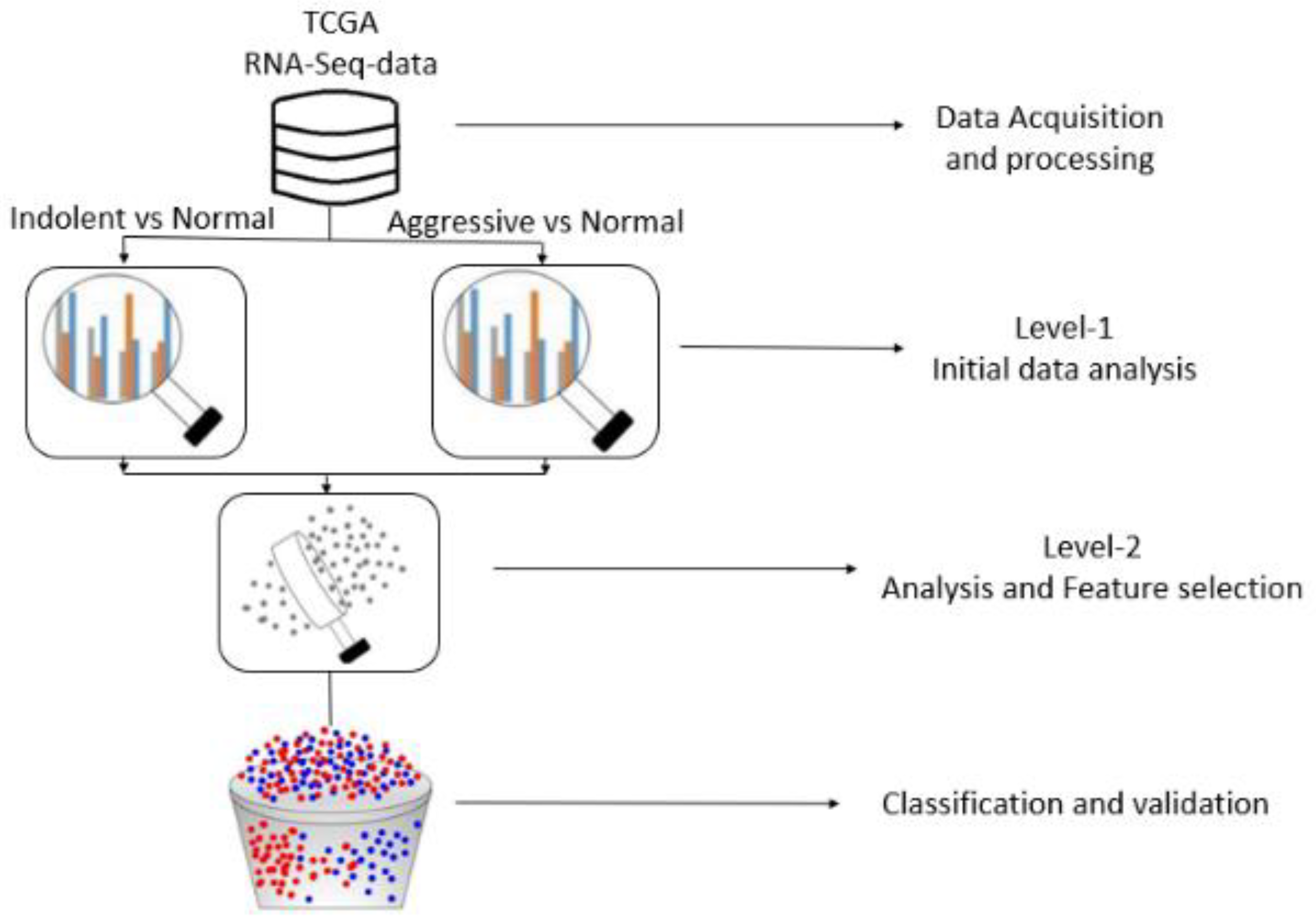
2.2. Data Processing and Analysis for Gene Selection

We performed data quality control and processing steps for gene expression data containing 60,483 probes across 547 samples. The counts per million (CPM) filter (>0) was implemented in R (version 3.5.1) using the edgeR library to remove the rows with missing data (i.e., zero or very low gene expression values), such that each row had at least ≥30% of data [15,16]. After applying the filter, the resulting dataset had 34,956 probes across 547 samples. As shown in Supplementary Figure S1, all the library sizes of samples in TCGA data were expressed using a bar plot to determine if there were any major discrepancies among samples. This analysis aimed to identify any significant disparities among the samples. Subsequently, it became evident that the data quality was suboptimal and deviated from a normal distribution. To mitigate this issue, we performed an initial normalization step by applying a logarithmic scale transformation to the count matrix. This scaling technique is commonly used to address gene expression data’s inherent variability and dynamic range in RNA-Seq experiments [15,16]. By applying the log transformation, we aimed to achieve a more balanced and comparable distribution of gene expression values across samples. Box plots were used to check the read count distribution on the log2 scale. To address variations in library sizes among the samples containing gene expression data, we employed the CPM function to correct the data. This function calculates the log2 counts per million (log2 CPM) values, considering each sample’s total library size [15,16]. Additionally, a small offset was added to the log2 CPM values to mitigate the issue of excessive zeros in the dataset [15,16]. Supplementary Figure S2 represents the boxplots of logCPM (log counts per million) before normalization.
Composition biases were eliminated among libraries and generated a set of normalization factors (the product of the library sizes and factors defining the effective library size) using the Trimmed Mean of M-values (TMM) [15,16]. We then performed a Voom transformation and generated a mean–variance trend plot, as shown in Supplementary Figure S3, using R. For data analysis, we used the Limma package implemented in R, which offers the Voom function that transforms the read counts into logCPM and has been successfully used by our group and others [17,18]. Then, the multi-level data analysis was performed as described below.

2.2.1. Level 1 Analysis

Using normalized data, we performed level 1 analysis comparing gene expression levels between tumor samples and controls for indolent and aggressive PCas separately using the Limma package in R [17,18]. This baseline was used for analysis to discover the signature of genes/features significantly (p < 0.05) associated with each type of disease. A volcano plot was used to visualize the results. We used the false discovery rate (FDR) procedure to correct for multiple-hypothesis testing [16]. The probes were ranked on p-values and −log fold change (−log FC). Significantly differentially expressed genes/features between tumors and controls were associated with each type of PCa.

2.2.2. Level 2 Analysis

Following the discovery of genes associated with each subtype of PCa from level 1 analysis, we created a new gene expression dataset containing genes significantly associated with indolent and aggressive PCas. Then, several analysis strategies were performed on the combined dataset to identify significantly differentially expressed genes to distinguish indolent from aggressive PCas. First, we compared gene expression levels between patients with GG 6 and GGs 8–10. Second, because GG 7 follows a variable clinical course, we compared gene expression levels between patients with GGs 6 and 7 (3 + 4), and patients with GGs 8–10 and 7 (4 + 3). (Note that individuals with GG 7 assigned a pathological score of 3 + 4 were considered GG6; similarly, individuals with GG 7 assigned a pathological score of 4 + 3 were considered GGs 8–10 [14]). Thirdly, we compared gene expression levels between patients presenting with GG 7 assigned a pathological score of 3 + 4 and patients with GG 7 assigned a pathological score of 4 + 3. We computed the p-values and the –log fold change (−logFC) for each analysis. The FDR procedure was used to correct multiple-hypothesis testing [16]. The genes/features were ranked on p-values and –logFC. Sets of significantly differentially expressed genes between indolent and aggressive PCas from each analysis were used as the features in the development and implementation of classification algorithms.

2.2.3. Feature Selection and Implementation of ML and Genetic Algorithms

Developing, applying, and evaluating ML classifiers involved selecting genes or features from gene expression data analysis using different cutoffs. The cutoffs were determined according to the p-values and logFC values of significant genes identified in the analyses. We selected features at different threshold levels based on −logFC > 0.5, 0.7, 1, 1.5, and 2 to test and validate the classification algorithms. Because ML algorithms can perform differently, we selected five different classifiers implemented with different fundamental approaches: Logistic Model Tree (LMT), MultiClassClassifier, Stochastic Gradient Decent (SGD), Sequential Minimal Optimization (SMO), SimpleLogistic [19]. We used Weka 3.8.2 software to implement the algorithms [19]. A 10-fold cross-validation technique was used on all mentioned subsets to prevent overfitting, with metrics averaging over all 10 folds and being tested on each classifier. Apart from traditional feature selection using logFC and p-value, we also implemented a Genetic Algorithm (see Supplementary Figure S4) to extract important features from a subset (abs(logFC) > 0.5). Using the set of identified features, we tested the seven classifiers listed and described below [19,20]:
(1)
Support Vector Machine (SVM).
(2)
Logistic Regression (LR).
(3)
Random Decision Forest (RF).
(4)
Extra Tree Classifier (ETC).
(5)
Gradient Boosting Classifier (GBC).
(6)
K-Nearest Neighbors (KNNs).
(7)
eXtreme Gradient Boosting (XGB).
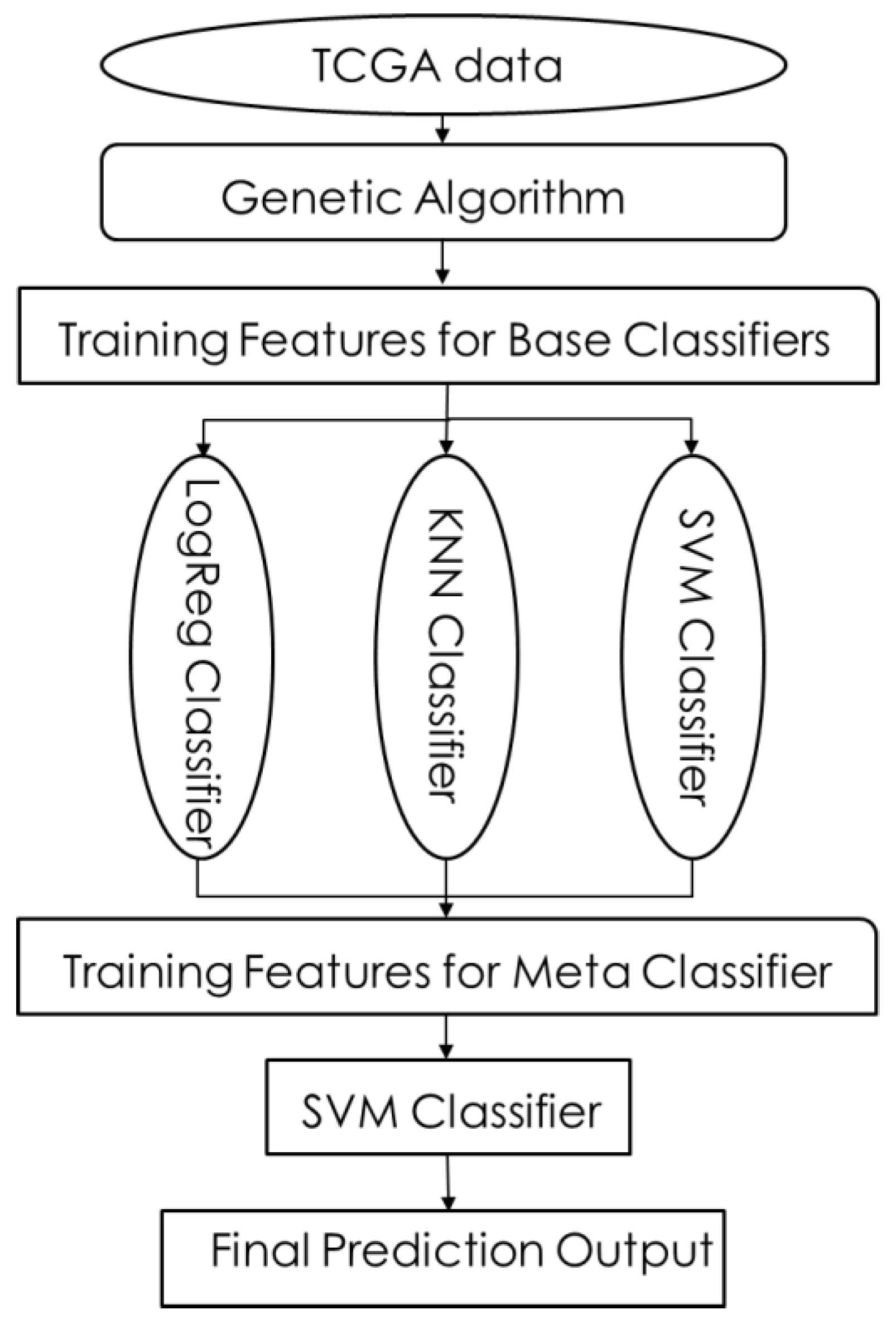
(i) Support Vector Machine (SVM): SVM [21] is a machine learning classifier, which is defined by a separating hyperplane in an N-dimensional space that classifies each data point (where N is the number of features). Hyperplanes help in classifying data points and depend upon the number of features. If the number of features in a dataset is 2, then the hyperplane is just a line. If the number of features in a dataset is 3, then the hyperplane is a plane. If the number of features is greater than 3, then it would be difficult to imagine a hyperplane.
(ii) Logistic Regression (LR): Logistic Regression [22] is a technique for analyzing data that determines the dependent output (outcome) when there are one or more independent variables. In several cases, the outcome variable (dependent) is a dichotomous variable in which there are only two possible outcomes. The goal is to find the best-fitting model to describe the relationship between the dependent variable and the set of independent variables. The logistic sigmoid function is used to return a probability value by transforming the output, which can be mapped to discrete classes. Regularization techniques are used to avoid overfitting (any modification made to a learning algorithm is intended to reduce the generalization error).
(iii) Random Decision Forest (RF): Random Decision Forest [23] is a supervised machine learning algorithm that randomly creates and merges more than one decision tree into a forest. During training time, the RF algorithm operates by constructing a multitude of decision trees and outputting the class that is a classification or mean prediction (regression) of individual trees. It adds additional randomness to the model by growing trees. The best feature is searched among a random subset of features instead of searching for the most crucial feature while splitting a node. Random Decision Forest is an effective approach for mitigating the issue of overfitting the training dataset. This technique addresses overfitting by constructing multiple decision trees on different subsets of the dataset. The collective predictions of these trees are then combined to form a mean prediction, which improves the overall accuracy of the forest and helps prevent overfitting.
(iv) Extra Tree Classifier (ETC): The Extra Tree [24] method is also known as extremely randomized trees. An Extra Tree Classifier’s main objective is to randomize the input features of a tree, where the large proportion of the variance of the induced tree depends on the choice of the optimal cut-point. It constructs randomized decision trees from the original learning samples and uses the above-average decision to improve accuracy and avoid overfitting. The method selects a cut-point at random and drops the idea of using bootstrap copies of the training sample. Cut-point randomization often reduces the variance when the bootstrapping idea is dropped and can also lead to an advantage in terms of bias. This method has yielded state-of-the-art results in high-dimensional complex problems.
(v) Gradient Boosting Classifier (GBC): GBC [25] is a machine learning technique used for classification and regression problems. It builds a model in a forward-stage-wise fashion like other boosting methods. It allows for the optimization of arbitrary differentiable loss functions. It involves three elements: (a) a loss function to be optimized, (b) a weak learner to make predictions, and (c) an additive model to add weak learners to minimize the loss function. Gradient Boosting Classifier’s main objective is to minimize the model’s loss by adding weak learners in a stage-wise fashion using a procedure similar to that of gradient descent. While adding a new weak learner, the existing weak learners in the model remain unchanged. To correct or improve the final output, the output of a new learner is added to the existing sequence of learners.
(vi) K-Nearest Neighbors (KNNs): K-Nearest Neighbors [26] is an algorithm that classifies new cases based on a similarity measure of all stored available instances. It has been used as a non-parametric statistical estimation and pattern recognition technique. A case is assigned to the common class among the K-Nearest Neighbors, measured by a distance function, and classified by a majority vote of its neighbors. If k = 3, then the class is assigned to a class of its three nearest neighbors.
(vii) eXtreme Gradient Boosting (XGB): The implementation of eXtreme Gradient Boosting [27] offers several advanced features for model tuning, algorithm enhancement, and computing environments. It can perform in three different forms of gradient boosting (Gradient Boosting (GB), Stochastic Gradient Boosting (GB), and Regularized Gradient Boosting (GB)). It is strong enough to support fine tuning and the addition of regularization parameters. It uses regularized model formalization to avoid overfitting and results in better performance. Moreover, XGB trains faster compared with other methods.
The following table (Table 1) shows the important parameters that are used to train the models using the seven classification algorithms.

2.2.4. Stacking

In addition to the above-described ML algorithms, we employed the stacking model explained below [28,29,30,31,32] to address the limitations of individual classification algorithms. The approach reduces the generalized error rate and increases accuracy by combining the prediction probabilities of the individual classification models [30,31,32]. Figure 2 shows the workflow for implementing the stacking approach. Two stages of learners were used to implement the stacking model. In the first stage of classifiers, base classifiers were used. In the second stage, meta-classifiers were used. To find the base and meta-classifiers for the first and second stages of the stacking framework, we examined the seven different machine learning algorithms described above, whose characteristics are defined below, and performed the five different stacking models listed below. The models were built and optimized using Scikit-learn [33]. We used three different models, as explained earlier in this section. The below-mentioned stacking models (SM-1, SM-2, SM-3, SM-4, and SM-5) were performed using two different datasets:
(1)
SM-1: LR, KNNs, SVM as base classifiers; SVM as meta-classifier.
(2)
SM-2: LR, SVM, KNNs, XGB as base classifiers; XGB as meta-classifier.
(3)
SM-3: LR, KNNs, SVM as base classifiers; XGB as meta-classifier.
(4)
SM-4: RDF, LR, KNNs as base classifiers; GBC as meta-classifier.
(5)
SM-5: RDF, LR, GBC as base classifiers; KNNs as meta-classifier.

2.3. Model Selection and Validation by Correlating ML Algorithm with GGs

To address our working hypothesis that genomic alterations in patients diagnosed with indolent and aggressive tumors could lead to measurable changes distinguishing the two patient groups, including GG 7, we implemented 3 models to find the best classifier. In Model 1, we selected all the samples with Gleason Grades 6 and 3 + 4 indolent versus Gleason Grades 8–10 and 4 + 3 aggressive at different threshold levels for all the log-fold change values of 0.5, 0.7, 1, 1.5, and 2. This model was based on the current classification protocol where samples with Gleason Grade 7 assigned with a pathological score of 3 + 4 are classified as indolent, whereas samples with Gleason Grade 7 assigned with a pathological score of 4 + 3 are classified as aggressive PCas, consistently with the American Urological Association guidelines [14]. Using features selected based on this model, we applied the seven ML methods described above to evaluate the classification of GGs. In Model 2, we used the samples with Gleason Grades 6 and 8–10 for all log-fold change values (0.5, 0.7, 1, 1.5, 2). Here, the samples with GG = 7 were removed, and the model was trained on Gleason Grade 6 (indolent) versus Gleason Grades 8, 9, and 10 (aggressive) tumors using the seven ML classifiers. In Model 3, we used samples with Gleason Grade 7 for all log-fold change values (0.5, 0.7, 1, 1.5, 2). The model was trained on Gleason Grade 7 (3 + 4) indolent versus Gleason Grade 7 (4 + 3) aggressive tumors using the seven ML classifiers. Because GG 7 follows a variable clinical course, we used Model 2 for training and correctly classified samples with GG 7 as a test set.

2.4. Performance Evaluation

We evaluated the performance of ML classifiers based on the results using two approaches. In the first approach, we created a set of classifier performance evaluation metrics, with their names and definitions being mentioned in Table 2 below. In the second approach, principal component analysis (PCA) plots were used to check if the samples were correctly classified as indolent and aggressive. We should see a clear separation of samples in the plot if the classifiers predicted them correctly. The evaluation metrics used are presented in Table 2.

3. Results

3.1. Discovery Genes Associated with Indolent and Aggressive PCas

To address the hypothesis that genomic alterations could lead to measurable changes associating gene expression to indolent and aggressive PCas, we separately compared gene expression levels between indolent tumors and controls, and between aggressive tumors and controls, as described in the Methods section under Level 1 Analysis. Comparing gene expression levels between indolent tumors and controls produced a signature of 18,215 (p < 0.05) differentially expressed genes. Repeating the same analysis comparing gene expression levels between aggressive tumors and controls produced a signature of 21,042 significantly (p < 0.05) differentially expressed genes.

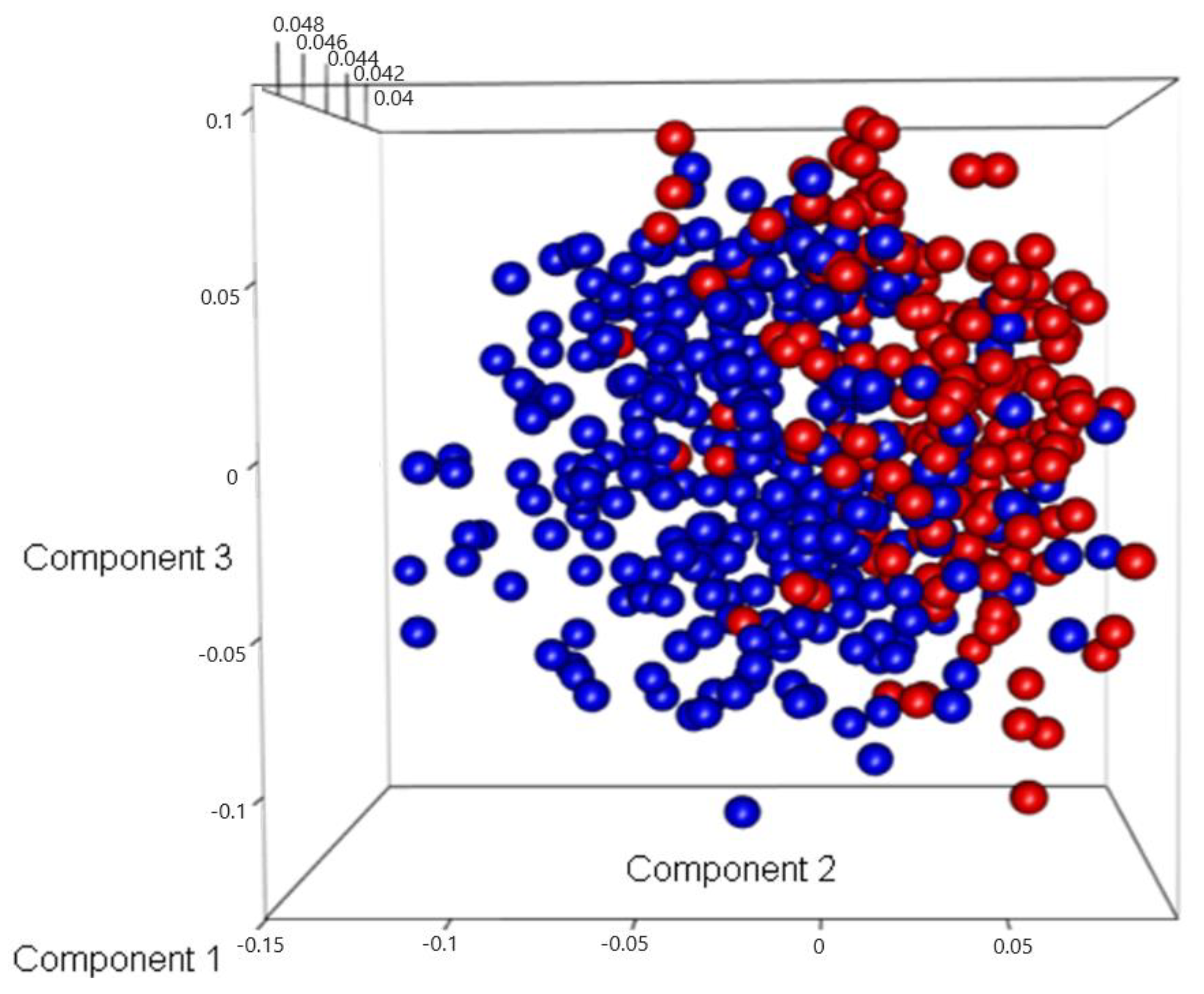
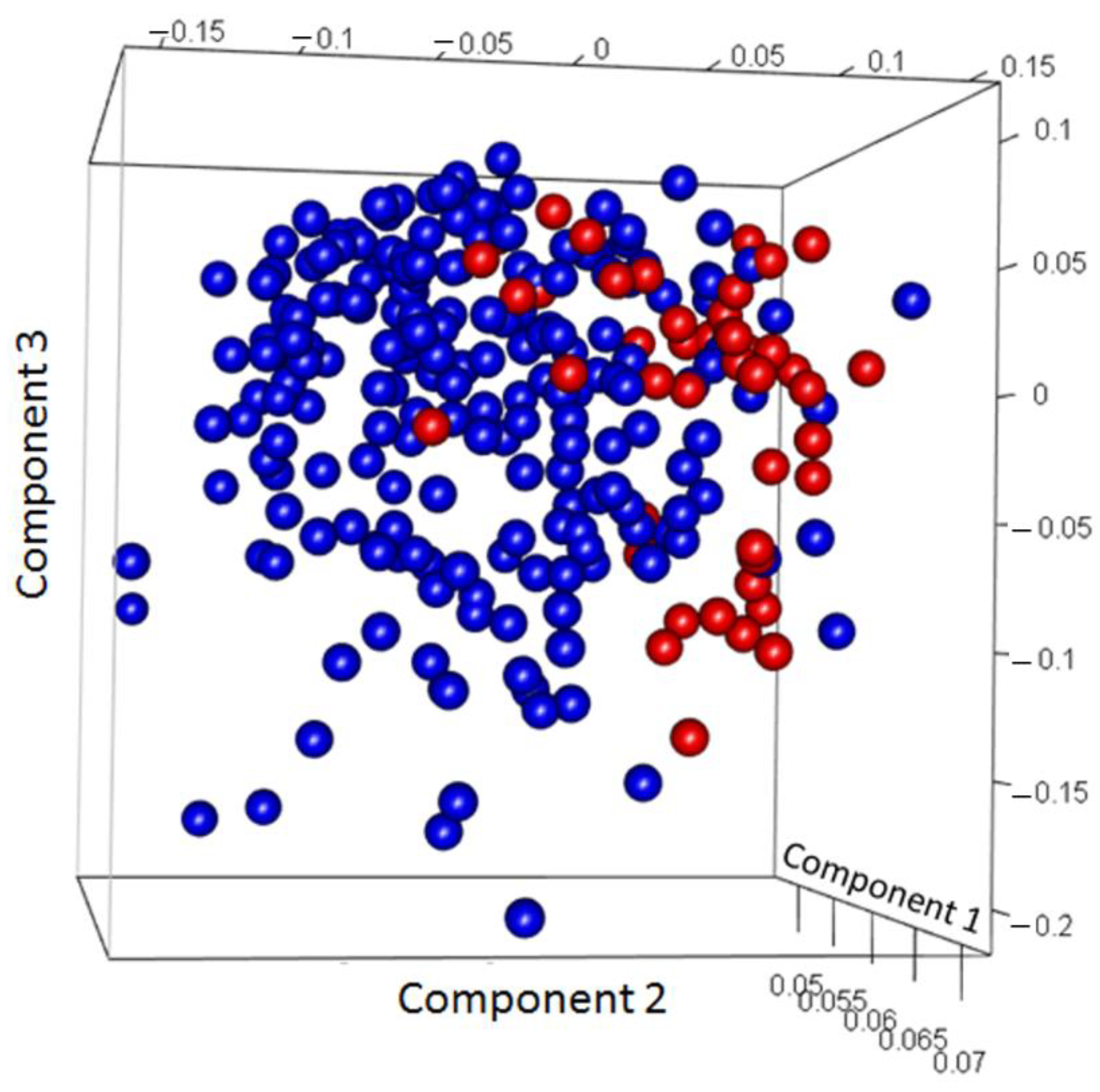
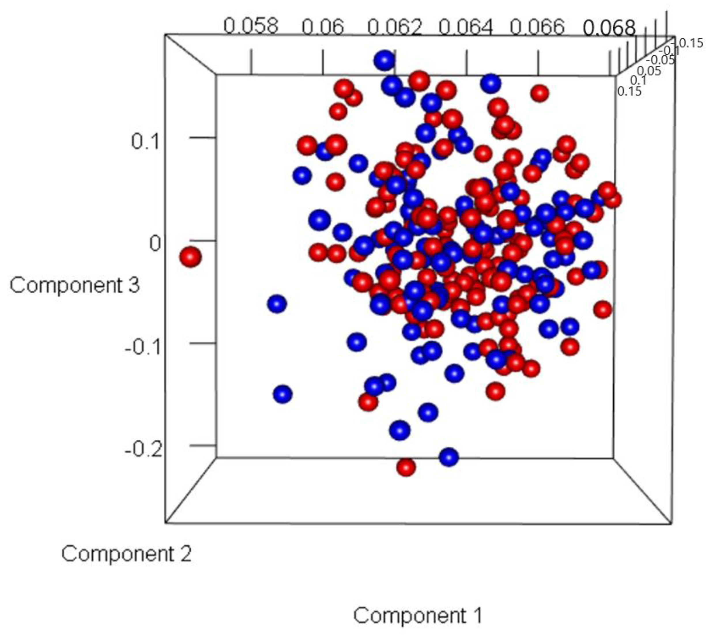
3.2. Discovery of Genes or Features Associated with the Two Types of PCa Used in ML Algorithms

To discover genes/features used in developing and validating classification algorithms, we performed a subgroup analysis based on three models as explained in the Methods section under Level 2 Analysis. In Model 1, we compared gene expression levels between patients with GG 6 and GGs 8–10 using the genes associated with the two diseases. The analysis conducted in Model 2 yielded 15,105 significantly (p < 0.05) and 20,712 significantly (p < 0.05) differentially expressed probes associated with indolent and aggressive PCas, respectively. We used volcano plots (Supplementary Figures S5–S7) to discover a signature of genes significantly (p < 0.05) associated with each disease state. In Model 2, because GG 7 follows a variable clinical course, we compared gene expression levels between patients with GGs 6, 7 (3 + 4) and patients with GGs 8–10, 7 (4 + 3). As described earlier in the Data Analysis section, individuals with GG 7 assigned a pathological score of 3 + 4 were considered GG6, and individuals with GG 7 assigned a pathological score of 4 + 3 were considered GGs 8–10 [14]. This model produced xx genes. In Model 3, we compared gene expression levels between patients presenting with GG 7 assigned a pathological score of 3 + 4, and patients with GG 7 assigned a pathological score of 4 + 3. This yielded 5220 significantly (p < 0.05) and 3352 significantly (p < 0.05) differentially expressed probes associated with indolent and aggressive tumors, respectively. We then compared indolent and aggressive PCas using the differentially expressed probes from the earlier analysis and used volcano plots to discover a signature of genes significantly (p < 0.05) associated with each disease state. A summary of genes or features discovered with Model 1–3 Differential Expression Analysis on indolent and aggressive diseases used in algorithm development and validation at different threshold levels as determined according to logFC is presented in Table 3.

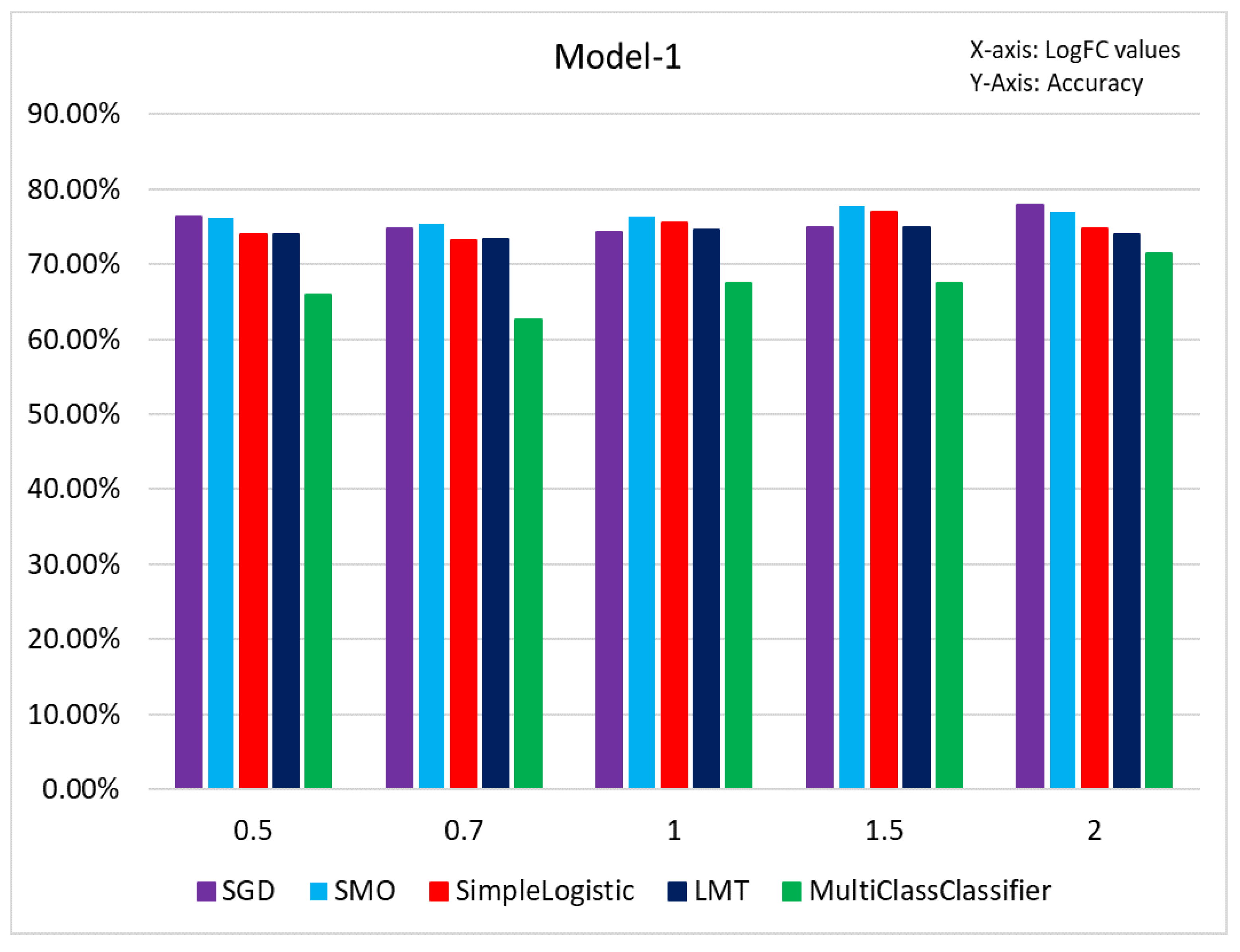
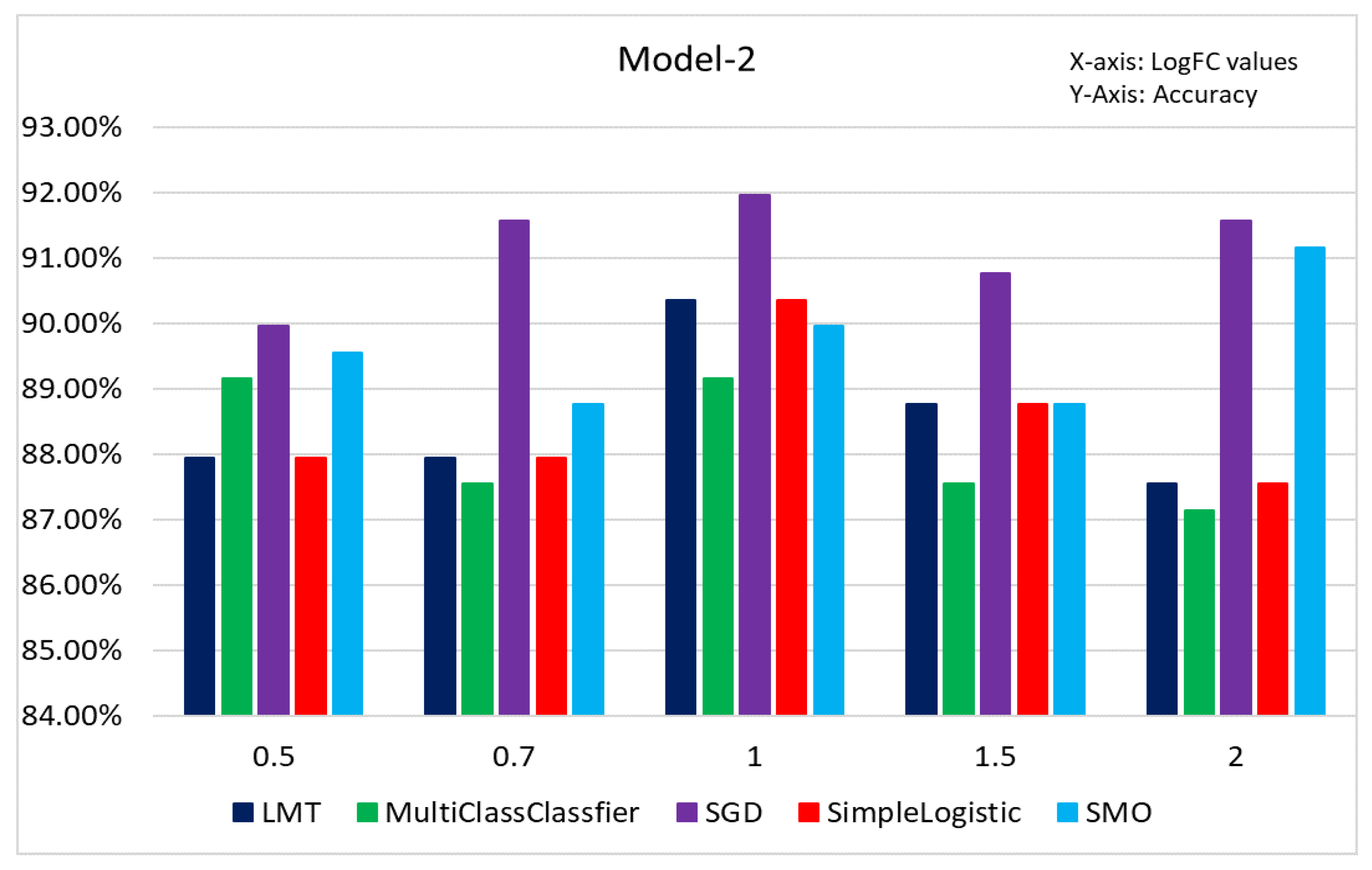
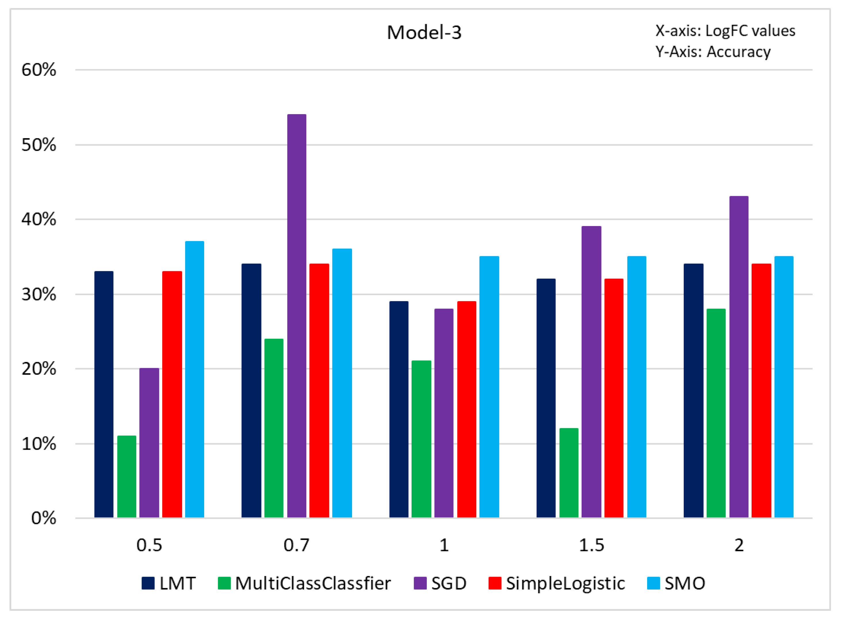
3.3. Results of Classification Based on Different Models

The object of this study was to evaluate the efficacy of ML algorithms for the classification of PCa patients into indolent versus aggressive PCas using gene expression data from TCGA. To address this objective, we evaluated different ML classification algorithms under different models (Models 1–3) using different sets of features selected using different threshold levels as determined with −logFC. ML classifiers included SVM, LR, RF, ETC, GBC, KNNs, and XGB. The results are summarized below.
In model 1 (full model), we considered all the samples with Gleason Grades 6–10 and applied ML classifiers at different threshold levels, abs(logFC) > 0.5, 0.7, 1, 1.5, and 2. The results of this investigation are presented in Figure 3 for the classification algorithms and in Figure 4 for principal component analysis, showing the separation between indolent and aggressive tumors. As shown in Figure 3, the SGD classifier achieved the highest accuracy at LogFC 2, 78.18%. MultiClassClassifier achieved the lowest accuracy at LogFC 0.7, 62.63%. Using a PCA plot to check if the samples were correctly represented as indolent and aggressive revealed a mixture and misclassification of samples (Figure 3). Most of the misclassification was attributed to GG 7.
In model 2, we removed the samples with GG 7 and applied machine learning classifiers to the remaining samples (GG 6 versus GGs 8–10) with different LogFC cutoffs. Here, we sought to address misclassification resulting from the inclusion of data from individuals diagnosed with GG 7. The results of this investigation are presented in Figure 5. The classification accuracy improved significantly, and the misclassification error was reduced. The SGD classifier obtained the highest accuracy at LogFC 1, 91.97%, and MultiClassClassifier obtained the lowest accuracy at LogFC 2, 87.15%. PCA analysis (Figure 6) revealed that most of the samples with GGs 6, 8–10 were correctly classified. Model 2 achieved significantly higher accuracy and lower misclassification rates than Model 1.
Because GG 7 follows a variable clinical course, in model 3, we examined an additional classification approach to further address the misclassification problem for samples with GG 7. Under this approach, we applied ML classifiers to 3 + 4 versus 4 + 3 samples using the same cutoffs as those used in Model 1 and Model 2. The results of this investigation are presented in Figure 7. The accuracy was significantly lower, and the misclassification rate increased significantly. PCA analysis (Figure 8) revealed that most of the samples with GG 7 were misclassified. Overall, the results of Model 3 achieved significantly lower accuracy and higher misclassification rates compared with Models 1 and 2, further confirming the part of our hypothesis that high misclassification was attributable to GG 7.
Having discovered that including GG 7 causes high misclassification rates, we applied 10-fold cross-validation to all the ML classifiers for samples with GG 7 at different threshold levels, abs(logFC) > 0.5, 0.7, 1, 1.5, and 2. The highest and lowest accuracy values were obtained with the SGD classifier at LogFC 0.7, 54%, and MultiClassClassifier at LogFC 0.5, 11%, respectively. Figure 9 shows that Model 3 was misclassified compared with Model 1 and Model 2.
We implemented a supervised machine learning method to classify Model 3 by treating it as the test set and Model 2 as the training set. The accuracy significantly improved at all LogFC values for all the five different classifiers. According to Figure 10, the highest and lowest accuracy values were obtained with MultiClassClassifier at LogFC 1.5, 87.55%, and the SimpleLogistic classifier at LogFC 2, 73.74%, respectively. According to Table 4, we can discern that the highest accuracy obtained by an individual classifier (SVM) using Scikit-learn was 86%.

3.4. Stacking Results

We increased the accuracy to 86% by correctly classifying samples with GG 7. A Genetic Algorithm (GA) was implemented to reduce the number of features to identify the genes/features that contribute to the disease. GAs are metaheuristics that gradually refine solutions using natural selection, where the best individuals are selected to produce offspring for the next generation. GAs are used to generate high-quality solutions to optimization by relying on operators such as selection, crossover, and mutation. In the optimization using the GA, the parameters were set as (i) population size of 50, (ii) elite rate of 5%, (iii) crossover rate of 90%, and (iv) mutation rate of 50%. Figure 2 represents the stacking method. After applying the Genetic Algorithm, the resulting models contained 1020 (Model 1) and 1681 (Model 2) genes. Later, we assumed that classifying with all the samples could increase our accuracy using both models.
Using stacking in Model 1, we evaluated different combinations of base classifiers and meta-classifiers using our stacking technique. Table 5 represents the performance metric of Model 1, and the highest accuracy was obtained with Stacking Model 1 (SM-1), 96%. Then, we used a principal component analysis (PCA) plot to check if the samples were correctly represented as indolent versus aggressive PCas. In Figure 11, we observe that most of the samples were correctly classified.
For the stacking method under Model 2, we removed the samples with GG 7 and applied the stacking technique with different combinations for the rest of the samples. The results are presented in Table 6. Model 2 is now more comparable to Model 1, and the highest accuracy was obtained with Stacking Model 1 (SM-1), 97%. Almost all the samples were classified correctly (Figure 12). Due to our model’s inability to achieve 100% accuracy, a few misclassified samples persisted within our models. Figure 9 shows the number of misclassified samples in GG7 and Model 1 at different threshold levels, abs(logFC) > 0.5, 0.7, 1, 1.5, and 2.

4. Discussion

The accurate classification of individuals diagnosed with PCa into those with indolent tumors that could be put under surveillance and those with aggressive diseases requiring immediate medical attention remains an unresolved challenge. Clinical oncologists face the dilemma of over-treating individuals with indolent tumors and under-treating individuals with aggressive tumors, with the potential consequence of bad clinical outcomes in either case. This study was undertaken to investigate the potential utility of ML algorithms for classifying PCa patients into patients with indolent tumors that could be safely monitored and patients with aggressive tumors with lethal potential that require immediate therapeutic intervention. Our investigation shows that using the current protocol based on GG scoring alone could lead to high misclassification errors. The practical consequence is that this could lead to unnecessary treatment of men with indolent tumors, a practice that could impair their quality of life and potentially their economic well-being. Likewise, under-treatment due to misclassification could lead to loss of life in those who could otherwise be saved. Our investigation shows that implementing ML algorithms could accurately classify cancer patients into patients with indolent and aggressive PCas. Our investigation also shows that while ML algorithms vary in their accuracy, using stacking methods that combine different ML algorithms could significantly increase the accuracy and reduce misclassification errors and could be used to complement current protocols based on GGs.
In our study, we used Differential Expression Analysis and a Genetic Algorithm to reduce the number of features to identify the probes contributing to the disease. We also performed different ML classifiers using 10-fold cross-validation to minimize the misclassification rate and improve accuracy compared with previous studies. Later, we used a stacking-based ML technique using a different combination of ML classifiers with 10-fold cross-validation and yielded better results (Model 1: 96% with SM-1; Model 2: 97% with SM-1). To validate and compare the performance of our stacking models, we compared their performance with that of existing methods. The following table (Table 7) compares the proposed method with the existing methods. As shown in Table 7, our proposed Model 1 at 96% and Model 2 at 97% were significantly superior to the existing ones.
Some limitations of the study: Transcriptomics, the study of gene expression, in prostate cancer (Gleason Grades) provides valuable insights into gene activity [5]. However, it is crucial to acknowledge that transcriptomics alone may not fully capture the complexities of prostate cancer and effectively characterize patients. Prostate cancer is a heterogeneous disease with diverse underlying molecular mechanisms [1]. While transcriptomics reveals gene expression patterns, other data types, such as mutations and epigenetics, are equally vital to shaping cancer development and progression [2]. Mutations in the DNA sequence can lead to abnormal protein functions, contributing to tumor formation. Identifying specific mutations associated with different Gleason Grades can offer valuable diagnostic and prognostic information. Epigenetic alterations, modifications in DNA without sequence changes, profoundly influence gene expression and impact prostate cancer cell behavior and treatment response. Understanding epigenetic patterns in various Gleason Grades can provide insights into the disease’s biology and potentially lead to targeted therapies [13]. An integrated approach is necessary to comprehensively understand prostate cancer, combining data from multiple sources, including transcriptomics, mutations, and epigenetics. This approach allows researchers to gain a more nuanced understanding of the disease, enabling improved patient characterization based on the underlying molecular features of their tumors. However, in this study, we did not consider these features. Moreover, working with TCGA data presents challenges due to its unbalanced-design nature, causing technical difficulties in managing data dimensionality and fitting models to a large number of variables. Many studies have encountered similar issues when working with TCGA datasets. Addressing these challenges is essential to ensure robust and reliable analyses and advance our prostate cancer knowledge. These areas will be the focus of future investigations.

5. Conclusions

Our research highlights the significance of genomic alterations in distinguishing patients with indolent and aggressive tumors. Machine learning (ML) has emerged as a powerful toolset, providing precision, specificity, and sensitivity in accurately identifying truly indolent tumors that can be safely monitored and aggressive tumors requiring immediate treatment. With a unique combination of ML classifiers, the stacking-based ML technique demonstrated remarkable accuracy, surpassing 96% in 10-fold cross-validation. While the classification accuracy is commendable, there is potential for further improvement by incorporating additional features derived from mutation and epigenetic data, which would enhance patient characterization. While transcriptomics provides valuable insights into gene activity in prostate cancer, it is equally important to consider other genetic factors, such as mutations and epigenetics. By integrating these additional data points, we can gain a more comprehensive understanding of the disease, ultimately enhancing our ability to characterize patients and guide personalized treatment strategies. In addition, we plan to assess the effectiveness of neural network models in our future research. These models could prove valuable in integrating genomic data with somatic mutation information to classify indolent and aggressive prostate cancers and identify the driving factors behind disease aggression using machine learning. We believe that the tool we have developed will be useful in advancing our understanding of prostate cancer.

6. Patents

No patents resulted from the work reported in this manuscript.

Supplementary Materials

The following supporting information can be downloaded at: https://www.mdpi.com/article/10.3390/make5040066/s1. The following supplementary figures for data analysis are included.

Author Contributions

Data collection and processing: Y.K.K.M. and T.K.K.M. Conception and design of the experiments: M.W.U.K., J.W., C.H. and M.T.H. Performing of experiments: Y.K.K.M. Data analysis: Y.K.K.M., T.K.K.M., M.W.U.K. and C.H. Contribution of reagents/materials/analysis tools: Y.K.K.M., M.W.U.K., C.H. and M.T.H. Writing of the paper: Y.K.K.M., T.K.K.M., M.W.U.K., J.W., C.H. and M.T.H. All authors have read and agreed to the published version of the manuscript.

Funding

This research was supported by internal funds from LSUHSC-School of Medicine Startup funds, and external funds from National Institute of Health and National Institute of General Medical Sciences USA (grant numbers 2U54GM104940-07 and 2P20GM121288-06), and National Center for Advancing Translational Sciences USA (grant number UL1TR003096). All the views expressed in this manuscript are those of the authors and do not represent the funding sources or agency.

Data Availability Statement

The code and data related to the development of PCa-Clf can be found here: http://cs.uno.edu/~tamjid/Software/PCA_Predict/PCa-Clf.zip (accessed on 26 September 2023). All the original DNA methylation data and clinical information used in this investigation are publicly available in TCGA (https://www.cancer.gov/about-nci/organization/ccg/research/structural-genomics/tcga) and downloadable via the Genomics Data Commons (https://gdc.cancer.gov/). Data generated from the analysis supporting the findings of this study are provided in supplementary tables in the Supplementary Materials accompanying this report.

Acknowledgments

The authors thank Louisiana State University Health Sciences Center School of Medicine and University of New Orleans for providing the environment and laboratory space used to execute this project. The authors also thank Anthony Michael Marchiafava and Dixon James Wingrove for thoroughly reviewing the manuscript.

Conflicts of Interest

The authors declare no conflict of interest.

References

  1. Rodney, S.; Shah, T.T.; Patel, H.R.; Arya, M. Key papers in prostate cancer. Expert Rev. Anticancer Ther. 2014, 14, 1379–1384. [Google Scholar] [CrossRef] [PubMed]
  2. Watson, M.J.; George, A.K.; Maruf, M.; Frye, T.P.; Muthigi, A.; Kongnyuy, M.; Valayil, S.G.; Pinto, P.A. Risk stratification of prostate cancer: Integrating multiparametric MRI, nomograms and biomarkers. Future Oncol. 2016, 12, 2417–2430. [Google Scholar] [CrossRef] [PubMed]
  3. Epstein, J.I.; Allsbrook, W.C., Jr.; Amin, M.B.; Egevad, L.L.; ISUP Grading Committee. The 2005 International Society of Urological Pathology (ISUP) Consensus Conference on Gleason Grading of Prostatic Carcinoma. Am. J. Surg. Pathol. 2005, 29, 1228–1242. [Google Scholar] [CrossRef] [PubMed]
  4. Epstein, J.I.; Allsbrook, W.C., Jr.; Amin, M.B.; Egevad, L.L.; ISUP Grading Committee. The 2014 International Society of Urological Pathology (ISUP) Consensus Conference on Gleason Grading of Prostatic Carcinoma: Definition of Grading Patterns and Proposal for a New Grading System. Am. J. Surg. Pathol. 2016, 40, 244–252. [Google Scholar] [CrossRef]
  5. Lavi, A.; Cohen, M. Prostate cancer early detection using psacurrent trends and recent updates. Harefuah 2017, 156, 185–188. [Google Scholar]
  6. Moyer, V.A.; U.S. Preventive Services Task Force. Screening for prostate cancer: U.S. Preventive Services Task Force recommendation statement. Ann. Intern. Med. 2012, 157, 120–134. [Google Scholar] [CrossRef]
  7. Lin, J.S.; O’Connor, E.A.; Evans, C.V.; Senger, C.A.; Rowland, M.G.; Groom, H.C. US Preventive Services Task Force evidence syntheses, formerly systematic evidence reviews. In Screening for Colorectal Cancer: A Systematic Review for the U.S. Preventive Services Task Force; Agency for Healthcare Research and Quality: Rockville, MD, USA, 2016. [Google Scholar]
  8. Yang, L.; Wang, S.; Zhou, M.; Chen, X.; Jiang, W.; Zuo, Y.; Lv, Y. Molecular classification of prostate adenocarcinoma by the integrated somatic mutation profiles and molecular network. Sci. Rep. 2017, 7, 738. [Google Scholar] [CrossRef]
  9. Danaee, P.; Ghaeini, R.; Hendrix, D.A. A deep learning approach for cancer detection and relevant gene identification. In Pacific Symposium on Biocomputing 2017; World Scientific: Singapore, 2017; pp. 219–229. [Google Scholar]
  10. Takeuchi, T.; Hattori-Kato, M.; Okuno, Y.; Iwai, S.; Mikami, K. Prediction of prostate cancer by deep learning with multilayer artificial neural network. Can. Urol. Assoc. J. 2019, 13, E145–E150. [Google Scholar] [CrossRef]
  11. Wulczyn, E.; Nagpal, K.; Symonds, M.; Moran, M.; Plass, M.; Reihs, R.; Nader, F.; Tan, F.; Cai, Y.; Brown, T.; et al. Predicting prostate cancer specific-mortality with artificial intelligence-based Gleason grading. Commun. Med. 2021, 1, 1–8. [Google Scholar] [CrossRef]
  12. Liu, J.; Lichtenberg, T.; Hoadley, K.A.; Poisson, L.M.; Lazar, A.J.; Cherniack, A.D.; Kovatich, A.J.; Benz, C.C.; Levine, D.A.; Lee, A.V.; et al. An integrated TCGA pan-cancer clinical data resource to drive high-quality survival outcome analytics. The Cancer Genome Atlas Research Network. Cell 2018, 173, 400–416.e11. [Google Scholar] [CrossRef]
  13. The Genomics Data Commons. Available online: https://portal.gdc.cancer.gov/ (accessed on 26 September 2023).
  14. Bekelman, J.E.; Rumble, R.B.; Chen, R.C.; Pisansky, T.M.; Finelli, A.; Feifer, A.; Nguyen, P.L.; Loblaw, D.A.; Tagawa, S.T.; Gillessen, S.; et al. Clinically Localized Prostate Cancer: ASCO Clinical Practice Guideline Endorsement of an American Urological Association/American Society for Radiation Oncology/Society of Urologic Oncology Guideline. J. Clin. Oncol. 2018, 36, 3251–3258. [Google Scholar] [CrossRef] [PubMed]
  15. Robinson, M.D.; Oshlack, A. A scaling normalization method for differential expression analysis of RNA-seq data. Genome Biol. 2010, 11, R25. [Google Scholar] [CrossRef] [PubMed]
  16. Li, J.; Witten, D.M.; Johnstone, I.M.; Tibshirani, R. Normalization, testing, and false discovery rate estimation for RNA-sequencing data. Biostatistics 2012, 13, 523–538. [Google Scholar] [CrossRef]
  17. Mamidi, T.K.K.; Wu, J.; Hicks, C. Interactions between Germline and Somatic Mutated Genes in Aggressive Prostate Cancer. Prostate Cancer 2019, 2019, 4047680. [Google Scholar] [CrossRef]
  18. Doyle, M.; Phipson, B.; Ritchie, M.; Doyle, M.; Dashnow, H.; Law, C. RNA-Seq Analysis in R. Available online: http://combine-australia.github.io/2016-05-11-RNAseq/ (accessed on 26 September 2023).
  19. Brownlee, J. How to Run Your First Classifier in Weka. Mach. Learn. Mastery. 2020. Available online: https://machinelearningmastery.com/how-to-run-your-first-classifier-in-weka/ (accessed on 26 September 2023).
  20. Kuchi, A.; Hoque, M.T.; Abdelguerfi, M.; Flanagin, M.C. Machine learning applications in detecting sand boils from images. Array 2019, 3–4, 100012. [Google Scholar] [CrossRef]
  21. Vapnik, V.N. An overview of statistical learning theory. IEEE Trans. Neural Netw. 1999, 10, 988–999. [Google Scholar] [CrossRef]
  22. Szilágyi, A.; Skolnick, J. Efficient Prediction of Nucleic Acid Binding Function from Low-resolution Protein Structures. J. Mol. Biol. 2006, 358, 922–933. [Google Scholar] [CrossRef]
  23. Ho, T.K. Random decision forests. In Proceedings of the Proceedings of 3rd International Conference on Document Analysis and Recognition, Montreal, QC, Canada, 14–16 August 1995; Volume 271, pp. 278–282. [Google Scholar]
  24. Geurts, P.; Ernst, D.; Wehenkel, L. Extremely randomized trees. Mach. Learn. 2006, 63, 3–42. [Google Scholar] [CrossRef]
  25. Friedman, J.H. Greedy function approximation: A gradient boosting machine. Ann. Stat. 2001, 29, 1189–1232. [Google Scholar] [CrossRef]
  26. Altman, N.S. An Introduction to Kernel and Nearest-Neighbor Nonparametric Regression. Am. Stat. 1992, 46, 175–185. [Google Scholar]
  27. Chen, T.; Guestrin, C. XGBoost: A Scalable Tree Boosting System. In Proceedings of the 22nd Acm Sigkdd International Conference on Knowledge Discovery and Data Mining, San Francisco, CA, USA, 13–17 August 2016. [Google Scholar]
  28. Gattani, S.; Mishra, A.; Hoque, T. StackCBPred: A stacking based prediction of protein-carbohydrate binding sites from sequence. Carbohydr. Res. 2019, 486, 107857. [Google Scholar] [CrossRef] [PubMed]
  29. Hu, Q.; Merchante, C.; Stepanova, A.N.; Alonso, J.M.; Heber, S. A Stacking-Based Approach to Identify Translated Upstream Open Reading Frames in Arabidopsis Thaliana. In Book A Stacking-Based Approach to Identify Translated Upstream Open Reading Frames in Arabidopsis Thaliana; Springer International Publishing: Berlin/Heidelberg, Germany, 2015; pp. 138–149. [Google Scholar]
  30. Iqbal, S.; Hoque, M. PBRpredict-Suite: A Suite of Models to Predict Peptide Recognition Domain Residues from Protein Sequence. Bioinformatics 2018, 34, 3289–3299. [Google Scholar] [CrossRef]
  31. Mishra, A.; Pokhrel, P.; Hoque, T. StackDPPred: A stacking based prediction of DNA-binding protein from sequence. Bioinformatics 2018, 35, 433–441. [Google Scholar] [CrossRef] [PubMed]
  32. Flot, M.; Mishra, A.; Kuchi, A.S.; Hoque, T. StackSSSPred: A Stacking-Based Prediction of Supersecondary Structure from Sequence. Protein Supersecondary Struct. Methods Protoc. 2019, 1958, 101–122. [Google Scholar]
  33. Pedregosa, F.; Varoquaux, G.; Gramfort, A.; Michel, V.; Thirion, B.; Grisel, O.; Blondel, M.; Prettenhofer, P.; Weiss, R.; Dubourg, V.; et al. Scikit-learn: Machine Learning in Python. J. Mach. Learn. Res. 2012, 12, 2825–2830. [Google Scholar]
  34. Casey, M.; Chen, B.; Zhou, J.; Zhou, N. A machine learning approach to prostate cancer risk classification through use of RNA sequencing data. In International Conference on Big Data; Springer International Publishing: Cham, Switzerland, 2019; pp. 65–79. [Google Scholar]
Figure 1. Flowchart depicting study design and execution workflow. Only the genes significantly differentially expressed between tumors and controls discovered in the level 1 analysis were considered in the level 2 analysis.
Make 05 00066 g001
Figure 2. The flowchart represents the implementation of the stacking approach incorporating different combinations of ML algorithms.
Make 05 00066 g002
Figure 3. The figure represents the accuracy percentage of Model 1 before classification.
Make 05 00066 g003
Figure 4. Three-dimensional principal component analysis (PCA) plot of Model 1. (Here, blue represents indolent samples, and red represents aggressive samples).
Make 05 00066 g004
Figure 5. The figure represents the accuracy percentage of Model 2 before classification.
Make 05 00066 g005
Figure 6. Three-dimensional principal component analysis (PCA) plot of Model 2. (Here, blue represents indolent samples, and red represents aggressive samples).
Make 05 00066 g006
Figure 7. The figure represents the accuracy percentage samples with GG 7 before classification. Here, the x-axis represents log fold change values, and the y-axis represents accuracy.
Make 05 00066 g007
Figure 8. Principal component analysis (PCA) plot of Model 3. (Here, blue represents indolent samples, and red represents aggressive samples).
Make 05 00066 g008
Figure 9. Figure representing the misclassified instances in samples from both datasets (samples with GG 7 and samples with GGs 6–10).
Make 05 00066 g009
Figure 10. After classifying only samples with GG 7 with 5 different classifiers at different log-fold change values, the figure represents all the samples’ accuracy.
Make 05 00066 g010
Figure 11. The figure represents the principal component analysis of Model 1.
Make 05 00066 g011
Figure 12. The figure represents the principal component analysis of Model 2.
Make 05 00066 g012
Table 1. Selected hyperparameters of machine learning methods.
SVMLRRFETCGBCKNNsXGB
C = 1.0penalty = “l2”n_estimators = 100n_estimators = 100n_estimators = 100n_neighbors = 5n_estimatorst = 100
kernel = “rbf”tol = 1 × 10⁻⁴ criterion = “gini”criterion = “gini”loss = “log_loss”weights = “uniform”learning_rate = 0.3
gamma = “scale”C = 1.0max_depth = Nonemax_depth = Nonelearning_rate = 0.1algorithm = “ball_tree”max_deptht = 10
Table 2. Names and definitions of the evaluation metrics.
Name of MetricDefinition
True positive (TP)Correctly predicted positive samples
True negative (TN)Correctly predicted negative samples
False positive (FP)Incorrectly predicted positive samples
False negative (FN)Incorrectly predicted negative samples
Recall/sensitivity/true positive rate (TPR) T P T P + F N
Specificity/true negative rate (TNR) T N T N + F P
Fall-out rate/false positive rate (FPR) F P F P + T N
Miss rate/false negative rate (FNR) F N F N + T P
Accuracy (ACC) T P + T N F P + F P + T N + F N
Balanced accuracy (Bal_ACC) 1 2 ( T P T P + F N + T N T N + F P )
Precision T P T P + F P
F1 score (harmonic mean of precision and recall) 2 T P 2 T P + F P + F N
Mathews correlation coefficient (MCC) ( T P × T N ) ( F P × F N ) ( T P + F N ) × ( T P + F P ) × ( T N + F P ) × ( T N + F N )
Table 3. Distribution of the number of genes according to −logFC values for Models 1–3.
LogFC CutoffNo. of Genes
Model 1Model 2Model 3
0.520743513513
0.78212028381
1213836174
1.52418625
23525
Table 4. Performance of various classifiers in Model 1 after classifying samples with GG 7. The best score values are bold-faced.
Metric/
Method
LRETCKNNsSVMGBCRFXGB
Sensitivity0.850.930.860.910.910.920.90
Specificity0.670.490.590.690.540.510.67
Bal. acc.0.760.720.720.900.720.710.80
Accuracy0.800.820.790.860.820.820.85
Precision0.880.840.860.900.860.850.89
F1 score0.870.880.860.900.880.880.89
MCC0.500.840.450.610.490.490.61
Table 5. Performance of various stacking methods for Model 1. The best score values are bold-faced.
Method/
Metric
SensitivitySpecificityAccuracyPrecisionF1 ScoreMCCBalanced
Accuracy
SM-10.990.850.960.950.970.880.92
SM-20.960.830.930.950.950.810.87
SM-30.970.840.930.950.960.840.91
SM-40.980.680.910.900.940.740.83
SM-50.940.810.910.940.940.740.87
Table 6. Performance of various stacking methods for Model 2. The best score values are bold-faced.
Method/
Metric
SensitivitySpecificityAccuracyPrecisionF1 ScoreMCCBalanced
Accuracy
SM-10.980.900.970.990.980.870.94
SM-20.950.790.940.970.960.720.91
SM-30.960.790.950.970.970.720.92
SM-40.980.620.940.950.960.660.80
SM-50.980.590.930.950.960.640.78
Table 7. Performance comparison with existing methods.
MethodAccuracy
Yang et al. [8]82.54%
Danaee et al. [9]89.13%
Casey et al. [34]85.00%
Proposed Method (SM1) 96.00%
Proposed Method (SM2) 97.00%
Disclaimer/Publisher’s Note: The statements, opinions and data contained in all publications are solely those of the individual author(s) and contributor(s) and not of MDPI and/or the editor(s). MDPI and/or the editor(s) disclaim responsibility for any injury to people or property resulting from any ideas, methods, instructions or products referred to in the content.

