Identifying the Regions of a Space with the Self-Parameterized Recursively Assessed Decomposition Algorithm (SPRADA)

Abstract

This paper introduces a non-parametric methodology based on classical unsupervised clustering techniques to automatically identify the main regions of a space, without requiring the objective number of clusters, so as to identify the major regular states of unknown industrial systems. Indeed, useful knowledge on real industrial processes entails the identification of their regular states, and their historically encountered anomalies. Since both should form compact and salient groups of data, unsupervised clustering generally performs this task fairly accurately; however, this often requires the number of clusters upstream, knowledge which is rarely available. As such, the proposed algorithm operates a first partitioning of the space, then it estimates the integrity of the clusters, and splits them again and again until every cluster obtains an acceptable integrity; finally, a step of merging based on the clusters’ empirical distributions is performed to refine the partitioning. Applied to real industrial data obtained in the scope of a European project, this methodology proved able to automatically identify the main regular states of the system. Results show the robustness of the proposed approach in the fully-automatic and non-parametric identification of the main regions of a space, knowledge which is useful to industrial anomaly detection and behavioral modeling.

1. Introduction

The fourth industrial revolution, known as Industry 4.0, proposes to rethink the way the industrial sector is managed and controlled [1], by extending the areas of the Internet of Things (IoT) [2] and Artificial Intelligence (AI) [3] to traditional industry. Now, large, specialized machines are being replaced by smaller, possibly versatile production units, whilst the supply chain trades its conveyor belts for small, highly mobile robots [4]. The addition of intelligence to a hyper-connected system is expected to improve the autonomy of the units [5], and global efficiency more broadly [6], by making them react automatically in case of need (e.g., in case of disruption, change in the production schedule, etc.).

The most noticeable aspect of Industry 4.0 is the Industrial Internet of Things (IIoT), a topic which consists of connecting many systems within a wireless network, and investigating how to make them communicate. This can be achieved by using classical IoT tools (self-sufficient systems on chip, low-energy communication protocols, etc.) [7], or through a dedicated interface, for instance by using a Cyber-Physical System (CPS) [8].

Moreover, having many free-moving, possibly autonomous robots performing their tasks in parallel makes the investigation of solutions to manage them all at the same time a necessity. Such tools may allow them to collaborate [9], to decide which path to take to reach a place without injuring any system or people [10], to avoid collisions [11], etc.

Additionally, another major challenge of Industry 4.0 is the virtualization of systems, called digital twin, which aims to build an accurate and faithful representation of them [12]. Such tool can serve many purposes: modeling for anomaly detection [13], simulation for predictive maintenance [14], pure modeling and prediction for simulation [15], etc.

Actually, all these areas of research are different sides of the same challenge: the deep understanding of the industrial systems, so as to ameliorate their management and control. Indeed, intelligence often relies on information [16], for instance in the form of knowledge, which may be derived from the system’s processes, and especially their time series [17]. With real industrial systems, it may be automatically extracted from the processes’ historical data or human expertise by data-driven, machine learning-based approaches [18]. In that context, the extraction of knowledge seems to constitute the very first step of the emergence of a true intelligence [19]. Such knowledge can take many shapes: smart scheduling of the production orders to improve efficiency [20], modeling and prediction of time series for simulation [21], behavioral modeling to better understand and predict systems [22], etc.

In industry, in the scope of the predictive maintenance [23], a major challenge is the detection and diagnosis of anomalies [24], which, if not handled and corrected rapidly, may cause a more severe disruption or a true failure thereafter [25]. In industrial contexts, anomaly detection is often performed by machine learning or deep learning [26], especially using supervised algorithms, i.e., data must be labeled in some fashion upstream; however, obtaining such prior knowledge is often difficult, tedious and costly, since it typically requires manual investigation. On the contrary, data mining deals with the automatic extraction of knowledge from raw, unlabeled data, which makes it appealing as a possible candidate for anomaly detection [27]. In particular, unsupervised clustering may be greatly useful in such a context; clustering is commonly used in exploratory data analysis to find the main regions of a space [28], and can be applied to industrial contexts to isolate both the anomalies and the regular states of real unknown systems [29]. Indeed, this technique of statistical data analysis aims to regroup data sharing similarities with each other, whilst isolating the so-build groups from one another; with real system’s feature space, both the regular states and the historically-encountered anomalies should form compact groups, likely isolated from one another: clustering appears to be a relevant tool to separate the different groups automatically. Once the groups are isolated, they can easily be tagged as either anomalies or true regular states (that one may call the regular system’s “behaviors”), and can later on be used to feed any supervised classifier or predictive tool [30].

Although unsupervised clustering performs the task of separating the different groups of data within a space well, most of the related techniques are parametric: they require some prior information to correctly set the parameters before they can be performed [31]. Correctly setting them is essential to obtain a meaningful partitioning of the space [32]. Particularly, a parameter which is often required is the objective number of clusters to build: it greatly impacts the accuracy of the partitioning, and the relevance of the groups. Nevertheless, it is generally hard to set without accessing any prior knowledge on the system, thus, manual expertise is typically performed upstream [33]. Some clustering algorithms do not require that knowledge directly, by building the clusters one after the other until every data has been processed. However, such algorithms generally trade the number of clusters to be built by another parameter, which typically takes the form of a threshold, which determines the number of clusters issued, and thus the meaningfulness of the partitioning.

In order to accurately separate the different groups, one should feed the clustering algorithms with the correct objective number of clusters; nonetheless, there is no true solution to estimate that value without upstream manual processing. Additionally, the grain of the desired partitioning (i.e., comprising only the regular states, or also the anomalies within smaller groups) will affect that value: it is difficult to answer the question “how many behaviors and anomalies are contained within this N-month long dataset?” with absolute certainty, and especially in a fully automatic and blind fashion.

For that reason, this paper introduces a new unsupervised clustering methodology, specifically crafted to answer the above-mentioned difficulty of setting the objective number of clusters. This method consists of recursively splitting a space according to a split criterion: the space is partitioned a first time, then each cluster is analyzed using an integrity criterion, and, if it obtained a bad score, the cluster is itself split, and so on until the integrity of every issued cluster is acceptable. Once all the clusters are built, a final, small step of cluster merging is operated to fuse the smallest groups (especially that with one single data) into the largest ones. This method is self-parameterized, and is therefore named SPRADA, standing for Self-Parameterized Recursively Assessed Decomposition Algorithm. Notice that the objective number of clusters still matters, but considerably less, since if this value is not correctly set, then a dedicated step of clustering will be applied to compensate it.

The proposed method is applied to real industrial data, obtained in the context of an Industry 4.0-oriented European project; it proved to be accurate in identifying the main regions of the feature space, while also isolating the historical anomalies. These observations make the SPRADA method appealing for future work in the scope of predictive maintenance, alongside the development and deployment of Industry 4.0 solutions.

The manuscript is composed as follows: Section 2 is a detailed review of the literature on anomaly detection, the techniques to estimate the number of clusters of a dataset and the clustering techniques which do not require it. Then, the tools necessary for the proposed methodology are presented in Section 3, and the proposed SPRADA method is introduced and detailed in Section 4, and it is applied to a real industrial dataset in Section 5 to assess its accuracy and representativeness, and the findings are discussed in Section 6. Finally, Section 7 concludes this study.

2. State-of-the-Art

First, a short review of recent works about anomaly detection in industrial contexts is worth exploring to set the background of this study. To that end, several data-driven techniques were used, mostly based on deep learning, and especially on Convolutional Neural Networks (CNNs). For instance, Ref. [34] proposed to feed labeled anomalies of real solar plants into a CNN to learn and predict them; the study was then extended in [35] to many more Artificial Neural Networks (ANNs). Similarly, Ref. [36] learned the modes of a real hydro-power turbine by using Variational Modal Decomposition (VCM) and used CNN-oriented auto-encoders to detect unusual behaviors. Moreover, Ref. [37] used Root Cause Analysis (RCA) to identify the root causes of defects in a real steel industry hot strip mill, and then semi-automatically labeled the identified events to feed them in more classical machine learning-based ANNs. Eventually, some works used the real-time data collected by a Supervisory Control and Data Acquisition (SCADA) system to detect possible measurement intrusion, by using a classical Long Short-Term Memory (LSTM) [38], or by using supervised classification to identify both normal and abnormal activities, and finally learn the possible intrusions using supervised machine learning-based approaches [39].

All these techniques perform well, achieving promising results in the identification and prediction of anomalies, but they are computationally demanding, require a significant amount of data (a typical limitation in deep learning), and are supervised. Therefore, they are not suited to the fully-automatic and blind identification of the distinct anomalies—and behaviors—of industrial systems. That being said, the proposed SPRADA methodology may serve as a first fully-automated and non-parametric pre-processing tool to identify the historical anomalies, which may later on be fed to the works mentioned in the previous paragraph, whence the necessity of such a tool, and the correct estimation of the true number of groups (both anomalies and behaviors) in real industrial processes’ datasets.

Several attempts were made to estimate the “optimal” number of clusters to build to obtain the most representative partitioning as possible. Actually, the optimal value is not always that which optimizes an integrity criterion (e.g., cluster’s variance, density, etc.), since, with most quantifiers, the best partitioning method would be that where every single datapoint is contained in a unique cluster (for instance, the variance of every cluster would be zero); nevertheless, this partitioning would be positively useless, for it brings no information on the system’s feature space. Therefore, the techniques aiming to estimate the optimal number of clusters endeavor to provide a value which optimizes the integrity criterion of the clusters, whilst also maximizing the information brought by the partitioning (its meaningfulness).

Most of the techniques operate in an experimental fashion, by operating clustering several times, then evaluating the relevance of the partition (according to any criterion), and eventually estimating the optimal number of clusters to build as the value which provides a good trade-off between the accuracy and the size/number of clusters.

Among the techniques of the literature, probably the most widespread, albeit aging, is the Elbow method [40], which operates a given clustering algorithm several times, each time with a different value for the number of clusters, plots the explained variance of the clusters against the objective number of clusters, and eventually provides as optimal value that at the curve’s knee (or “elbow”), i.e., the point where the slope significantly changes. For instance, the Elbow method was used in [41] to automatically categorize the headlines from one thousand websites, and led to the identification of 7–8 major types of news, a pertinent piece of information to ease the research for readers. Nonetheless, the problem with this method is twofold: first, the curve’s knee is only an estimate, not an optimum, and a debate about the relevance of this point is discussed [42]; then, this method is essentially empirical, and not efficient, since the clustering algorithm must be executed several times to draw the curve whose knee must be found. Therefore, the Elbow method is essentially a sophisticated fashion to select the best partitioning among several of them, and not truly a way to provide an estimate for the optimal number of clusters.

Similarly, some methods trade the explained variance to more elaborated indicators, while keeping the same methodology than the Elbow method (i.e., finding the number of clusters which best maximizes the integrity of the clusters, while also providing a meaningful and representative partition of the feature space) [43]. Among others, some greatly popular criteria are the silhouette coefficients, which are integrity indicators providing, for every datapoint, a score indicating how close it is from its same cluster’s neighbors and how distant it is from the other clusters’ data. This approach gave birth to a dedicated clustering method, named silhouette clustering [44], which proposes to converge toward an optimal clustering (in the sense of the silhouette coefficients) by exhaustively and iteratively swapping the clusters’ barycenters and any other data to see if any improvement is obtained by this swap [45]. An example of application can be found in [43], who simulated a dataset composed of a certain number of noisy Gaussian distributions, and endeavored to retrieve the number of groups using the silhouettes-based version of the Elbow method; they obtained very good results, but the main problem with this method is its computational heaviness [46], since the silhouette coefficients themselves take a long time to compute ($\mathcal{O}\left(N^2\right)$, with N the number of data), and the comparisons to every pair barycenter-data ($\mathcal{O}\left(kN\right)$, with k the number of clusters) are numerous. Therefore, the complexity of the algorithm is in $\mathcal{O}\left(k{N}^{3}i\right)$, with i the number of iterations before convergence, which does not make it well-suited to large datasets such as industrial ones.

In addition, another well-known method is the Gap statistic [47]. This exploratory analysis technique relies on a simulated ground truth, obtained by generating a reference dataset under the null hypothesis, i.e., with the same statistical characteristics than the original one. Then, both the original and simulated datasets are clustered with a same algorithm, with the same value set for the number of clusters, and the average dispersion (for instance the mean distance between any possible pair of points) of the clusters for both partitions are compared. This procedure is repeated for several values as number of clusters, and that leading to the lowest difference between the mean dispersion of both partitions is chosen as the optimal number of clusters to build. An example of their application is presented in [48], where the authors aimed to retrieve the number of groups in real reference datasets using the Gap statistic method; they obtained mitigated results though, mostly due to the parameters to set: when correctly setting the parameters, they were able to retrieve the correct number of groups, but, when the parameters slightly differed from their optimal values, they obtained poorer results, mostly due to close and overlapping groups. Nonetheless, although being deemed reliable [49], this technique suffers from two major drawbacks: its computational heaviness, and its empirical approach. Since several values of the number of clusters must be tested, it could be considered a more sophisticated method to select the best partitioning among others, rather than a true way to estimate the number of clusters in a dataset.

Finally, in order to estimate the number of clusters, the authors of [50] proposed the ECD test, a semi-empirical approach which operates in a split-and-merge fashion. To that end, the authors began by creating a cluster dataset (only once) using a large value for the number of clusters, resulting in possibly very small groups, which are later characterized by their Empirical Cumulative Distributions (ECDs), which are finally compared using the Hausdorff distance and linked to one another using region-growing clustering. By comparing the ECDs of the different groups, the idea is to regroup the clusters in the same region of the feature space (which are assumed to have similar features, and therefore close ECDs), which are eventually merged to empirically estimate the borders of the distinct regions of the space. The ECD test aims to estimate the true number of regions of the feature space, value which serves as an estimate for the optimal number of clusters. This technique has the advantage of performing the clustering only once, is computationally efficient, since it relies on simple comparisons (the ECDs and the Hausdorff distance), and proved to be accurate in the identification of the borders of the feature space of a real industrial dataset.

All these works aim to estimate the “optimal“ number of clusters for a clustering algorithm to build, either by following a semi-empirical approach or by a simpler selection of the best partitioning among a set; they are summarized in

Table 1. Recapitulation of the methods to estimate the number of clusters for unsupervised clustering.

Name	Advantages	Limitations
Elbow method [40]	Reference method; statistical analysis of the information provided by the clusters.	Curve’s elbow not always easy to find; requires to execute the clustering algorithm several times.
Silhouettes Elbow [43]	Silhouette coefficients accurate and representative; provides a good estimate of the number of clusters.	Idem Elbow method + silhouette coefficients very long and expensive to compute.
Gap statistic [47]	Very good estimates when correctly parameterized.	Computationally heavy; requires to execute the clustering algorithm several times.
ECD test [50]	Simple and efficient; good results with industrial processes; requires to execute clustering only once.	The threshold conditions the grain of the merging, thus the number of regions identified.

to provide an overview of their advantages and limitations. However, some unsupervised clustering techniques are specifically crafted to perform without this parameter, in order to avoid the intrinsic difficulty one may encounter in estimating it.

Probably the most common category of unsupervised clustering techniques which build the clusters automatically is Hierarchical Clustering [51,52]. Such algorithms typically regroup data, or groups of data, by proximity or similarity in a hierarchical fashion. For instance, with a given dataset, the distance between every pair of data is computed, and the data of the pair with the lowest distance are linked together, forming the very first cluster; then, the procedure is repeated, but this time replacing the two previous data by their mean. As a consequence, all data are linked to each other in a hierarchical fashion, and the clusters can be obtained by stopping the linkage procedure somewhere. Knowing where to cut the link between the data/groups is the major drawback of hierarchical clustering, since it relies on a threshold (cut when two data/groups are at a distance higher than this threshold). In practice, Hierarchical Clustering was used in [53] to extract the manufacturing bottlenecks of a real-world production system from the event logs only, allowing the operators to identify the corresponding bottlenecks in the real system; it was also used by [54] in a more Industry 4.0-oriented context to propose a hybrid cut criterion in the scope of the design of a Decision Support System (DSS) for 3D printers.

Another relevant unsupervised clustering algorithm which does not require the number of clusters to build is Region Growing [55]. The general approach of such techniques is to draw a point from the database, aggregate its neighbors to it, thus forming a true cluster, and repeat the aggregation with any data contained within; once there is no more data close enough to any data in the cluster, it is considered fully built and another one is started following the exact same procedure, starting from any yet-unprocessed data. Region growing often achieves good results, but it is highly sensitive to initialization, and a threshold is required to characterize what “neighborhood” means, i.e., what is the maximal distance between two datapoints to consider them neighbors. It is popular in the segmentation of regularly spaced data, in particular images [56] and point clouds [57], since the data representing a same object are often similar, and a sudden change in values likely means an actual change of objects; for instance, when operating in the color space of an image, if two neighboring pixels belong to a same object, they should have approximately the same colors, but if they represent different objects, their colors should greatly differ. Nonetheless, with industrial processes, data are generally evolving continuously: sudden changes are rare, except when a shutdown or a power-on order is executed; as such, region growing may not be the most appropriate solution for real, dynamic industrial processes.

Another very popular algorithm is the Density-Based Spatial Clustering of Applications with Noise (DBSCAN) [58] algorithm, which operates somehow by region growing, but with a dedicated initialization procedure. Indeed, according to this method, the density of a cluster is defined as the number of data contained within a given topology ball. Therefore, the algorithm searches for local groups of data whose density meets a given parameter (e.g., if a datapoint has enough neighbors at a distance below this parameter, then it is assimilated as the cluster’s seed), regroups all of them to form a “proto-cluster”, before expanding it step-by-step by considering the neighborhood of the added data. Among other applications, DBSCAN was used in [59] to detect and segment the planar objects of a 3D point cloud, and it obtained good results on both academic and real datasets. It was also used in more industrial-related contexts, such as in [60], in which they compared it to the K-Means in the automatic detection of the different types of tasks performed by automated guided vehicles; DBSCAN proved able to better pinpoint the real tasks historically executed by the vehicles, knowledge which may serve for anomaly detection as a possible future refinement.

DBSCAN generates good results, but has the disadvantage of relying on a threshold as the first clusters’ radius (delineating the neighborhood of the seeds), and can only use one value for the density. To compensate that limitation, another algorithm, the Ordering Points To Identify the Clustering Structure (OPTICS) [61] replaces the fixed value for the neighborhood by a maximal value, thus every cluster smaller than this maximal threshold is considered (resulting in possibly varying densities). The counterpart is that this leads more to hierarchically connected groups of data rather than a true partitioning. Moreover, even though the impact of the threshold is leveled, it still must be set. As examples, OPTICS was used in [62] to localize the defects of the rolling parts of real systems, obtaining fairly encouraging results, and was also applied to Wireless Sensor Networks to detect the outliers, to serve as a semi-automatic pre-processing tool [63].

All these techniques of unsupervised clustering do not require the objective number of clusters to perform; nonetheless, they all have their own drawbacks. Some are highly sensitive to initialization, some others trade the number of clusters of the more traditional clustering methods for a neighborhood threshold, which sill needs to be provided upstream, and conditions the number of clusters issued, and some others are more a way to build a network of clusters, whose inter-distances would be represented by the length of the edges, rather than a true partitioning. The main methods of unsupervised clustering introduced in this section are summarized in

Table 2. Recapitulation of the algorithms which do not require the number of clusters as parameter.

Name	Acronym	Advantages	Limitations
Hierarchical Clustering [51,52]	HC	Simple and intuitive; provides a good representation of the data distribution.	Not a true space partitioning; requires the threshold of where to cut the links.
Region Growing [55]	RG	Simple and efficient; performs well in image segmentation.	Sensitive to initialization; needs the maximal distance delineating the neighborhood of data.
Density-Based Spatial Clustering of Applications with Noise [58]	DBSCAN	Intuitive and generic; provides good results in real situations.	Idem RG + slightly higher complexity and fixed density threshold.
Ordering Points To Identify The Clustering Structure [61]	OPTICS	Improvement of DBSCAN with a dynamic density threshold.	Closer to a hierarchically ordered set of clusters than a true partitioning.

, where their advantages and limitations are shortly mentioned to provide an overview of these methods.

This detailed literature review shows that many methods exist to, on the one hand, estimate the optimal number of groups present in a given dataset, and, on the other hand, to propose clustering algorithms which would overcome that limitation, by operating in an iterative fashion. Nonetheless, most of the already-existing techniques are either a sophisticated manner to select the best partitioning among others (e.g., the Elbow method), are computationally heavy (e.g., the silhouette coefficients), or replace that knowledge by another as of a threshold. As such, there currently exists no reliable and non-parametric solution to automatically identify and extract the true regular states (the behaviors) of real unknown systems, whence the proposal of the SPRADA method.

3. Required Already-Existing Materials for the Proposed Methodology

The proposed methodology, the SPRADA method, aims to identify the main region of an unknown feature space, by using a recursive and self-assessed approach. The proposed solution does not introduce new concepts sensu stricto, for it is essentially a methodology, i.e., how to use already-existing tools to carry out the proposed behavioral identification. As a consequence, in order to carry out this study, some concepts must be introduced, in particular unsupervised clustering and the metrics to quantify the integrity of the clusters. These topics are the matter of the two following subsections.

In all the following, d refers to any mathematical distance (e.g., Euclidean), the data instances are represented by x, and the database is denoted as $\mathcal{D}$ and is defined by (1),

$$\mathcal{D}={\left\{x_i\right\}}_{i\in \left[\right[1,N\left]\right]},$$

(1)

with $N=\left|\mathcal{D}\right|$ the cardinal (size) of the dataset, the final set of clusters is defined by (2),

$$\mathcal{C}={\left\{{\mathcal{C}}_k\right\}}_{k\in \left[\right[1,K\left]\right]},$$

(2)

where K is the total number of clusters, with any cluster ${\mathcal{C}}_k$ typically defined by (3),

$${\mathcal{C}}_k=\left\{x\in \mathcal{D}|\underset{k^{\prime }\in \left[[1,K]\right]}{argmin}\left(d(x,p_{k^{\prime }})\right)=k\right\},$$

(3)

where $p_k$ is the representative of cluster ${\mathcal{C}}_k$, outputted by the learning stage.

3.1. Unsupervised Clustering

Unsupervised clustering is the task which consists in regrouping data sharing similarities with each other, while also separating those which do not. For instance, the data contained within a same cluster should be no more distant than a given value, but two data from two distinct clusters should be more distant. Notice that any mathematical distance may be used, possibly leading to small variations in the results; typically, it is the Euclidean distance which is used. Additionally, the notion of “closeness”, or “similarity“, depends on the space where clustering is being operated; typically, it is the feature space which is chosen for that purpose. In the case of a real industrial system, the feature space may be that spanned by the basis formed by all the sensors of the system.

Probably the most well-known unsupervised clustering algorithm is the K-Means (KM) [64] algorithm. Albeit naive, it is also the most intuitive fashion to regroup data. It starts by drawing K points from the database, the barycenters, then it associates any point of the database to the closest barycenter to form the groups, the clusters. Once they are built, the barycenters are updated as the clusters’ means, and the procedure is repeated. The learning stops when any criterion is achieved, for instance a maximal number of iterations, or once the barycenters change very little from a round to the next. However, the K-Means has two limitations: it is not computationally efficient, and is only able to separate linearly separable groups (at least, in an Euclidean space).

An accurate alternative to the K-Means is the Self-Organizing Maps (SOMs) [65] algorithm, which operate similarly, but adds a notion of neighborhood to the learning. Indeed, there are still K points drawn first and assimilated to the clusters’ barycenters, but now they are virtually linked to each other in the form of a grid. Then, the learning procedure consists of statistically learning from the dataset. To that end, a datapoint is randomly drawn, and every barycenter is attracted to it, by applying a learning function updating the position of the barycenters, to bring them closer to the data drawn. The update is the strongest for the closest barycenter, and its strength diminishes as the farther away the barycenters get, and the less connected to the first one they are (i.e., the update is stronger for the direct neighbors of the closest barycenter, is weaker for the neighbors of the neighbors, and so on). Although aging, the SOMs are still very popular for their accuracy and efficiency: for instance, they found practical applications in [66] to evaluate the quality of groundwater, and in [67] to track the metaloids contained in soils. The SOMs are very accurate, are computationally efficient (due to their statistical approach), and proved able to distinguish most regular states from real industrial datasets [30], which makes them appealing for the identification of the main regions of industrial processes with the SPRADA method.

The SOMs are very general, work well in many cases, but some local adjustments may increase their accuracy and representativeness: Geographical SOM (Geo-SOM) to take into account spatial dependency [68], Time-Adaptive SOM (TASOM) to use time-adaptive parameters [69], Growing SOM (GSOM) to use a self-growing map [70], etc.

A useful alternative may be the Bi-level SOM (BSOM), proposed in [71]. This variant was originally crafted to identify the true regular states of a real industrial system, by somehow averaging several SOMs. Indeed, the main drawback of any statistical approach is that they are often sensitive to initialization: the very first points drawn will greatly affect the results, and the meaningfulness of the final partitioning; however, it is often very difficult to judge the quality of a space partition without any prior knowledge, thus there is no real way to decide which SOM is the most representative, and even if there is any. Nonetheless, in general, two SOMs will result in close partitioning, or, at least, some motif should appear, but each may be correct to some extent if no ground truth or any knowledge is made available, especially in a blind, Data Mining-oriented context. To answer that question, a BSOM aims to take benefit from the self-organization capability of the SOMs to average several maps as one, by generating a set of several SOMs, and then projecting all of them into a final one, somehow representing a statistically averaged map. In real situations, the BSOMs proved to be more accurate than the original SOMs and the K-Means to automatically identify the regular states of a real industrial system (its behaviors) [71].

The three main methods discussed in this subsection are summarized in

Table 3. Recapitulation of the unsupervised clustering methods used in this study.

Clustering Methods	Acronym	Advantages	Drawbacks
K-Means [64]	KM	Simple and intuitive; often used as a reference algorithm.	Not efficient and unable to separate nonlinear databases.
Self-Organizing Maps [65]	SOMs	Fast, efficient and generally deal properly with nonlinearities.	Tends to split the main behaviors of industrial processes in pieces.
Bi-Level Self-Organizing Maps [71]	BSOMs	Good results when identifying the behaviors of industrial processes.	Anomalies often missed (drowned out in the main behaviors).

to provide an overview on their strengths and weaknesses. These three unsupervised clustering algorithms can all be used in the proposed SPRADA methodology, and their respective accuracy will be discussed in Section 5.4. The advantage of using fairly simple algorithms (compared to that of Table 2) is that they can be performed several times.

3.2. Quantification of the Integrity of the Clusters

Once unsupervised clustering has been applied, the issued groups can be characterized in some fashion. Several metrics may be considered to that purpose: data dispersion, cluster compactness, span, density, etc. Whilst the traditional mathematical moments (mean, standard deviation, etc.) provide good indicators, they are generally not sufficient to correctly quantify the quality of the groups; additionally, they do not take into account the possible relationship between the clusters themselves. Actually, two aspects are worth being considered: how the data contained within a given cluster are organized between each other, and how the clusters are positioned in relation to each other. Indeed, if the data contained within the same cluster are very compact (e.g., low standard deviation), but that the cluster is close to another one, itself compact, therefore, both may be merged. On the contrary, if a cluster comprises a lot of data, but that are widely scattered, the cluster may be worth being split into several more compact pieces. The best case would be to obtain highly compact groups (low standard deviation of the data contained within each), but also highly distant from each other; for instance, the maximal distance between two data of any cluster would be $\epsilon$, and the minimal distance between two data of two different clusters would be several times greater, such as $10\epsilon$. In such a case, the clusters would be easily distinguishable from one another; however, this rarely happens with real systems, the clusters are never as compact, nor as distant from each other, and overlaps often occur.

A very well-known metric used to estimate the quality of a partition is the silhouette coefficients (or just silhouettes) [72]; they are now quite old, but are still in use by many works, such as by silhouette clustering. The silhouettes are normalized scores (ranging from $-1$ to $+1$) which indicate if a datapoint is close to its same cluster’s neighbors, while also being distant from the data of the other clusters. To do so, for every datapoint x, the metric computes the mean distance avg, defined by (4), to each of its neighbors, then, for every other cluster, it computes the mean distance dis, defined by (5), between x and every datapoint of that cluster, and it finally compares the two values by subtracting both and by dividing by the minimum of both to normalize the score, as expressed by (6). The closer to $+1$, the closer the data to its neighbors and the more distant from the other clusters, and vice-versa for the closer to $-1$. The silhouettes generally provide a good indicator of the integrity of the whole partitioning, but take a long time to compute (complexity in $\mathcal{O}\left(N^2\right)$), and there are too many coefficients to consider them all, thus, usually, only statistics of them are used (such as the average of the silhouettes of the data comprised by a cluster). Nonetheless, the computational complexity of the silhouette coefficients makes them ill-suited to very large datasets, such as industrial ones.

$$\begin{array}{cc}\hfill \forall x_i\in {\mathcal{C}}_k,avg\left(x_i\right)& =\frac{1}{|{\mathcal{C}}_k|-1}\sum _{x_j\in {\mathcal{C}}_k\setminus \left\{x_i\right\}}d(x_i,x_j)\hfill \end{array}$$

(4)

$$\begin{array}{cc}\hfill \forall x_i\in {\mathcal{C}}_k,dis\left(x_i\right)& =\underset{\begin{array}{c}{k}^{\prime }\in \left[[1,K]\right]\\ k^{\prime }\ne k\end{array}}{min}\left\{\frac{1}{|{\mathcal{C}}_{k^{\prime }}|}\sum _{x_j\in {\mathcal{C}}_{k^{\prime }}}d(x_i,x_j)\right\}\hfill \end{array}$$

(5)

$$\begin{array}{cc}\hfill \forall x_i\in {\mathcal{C}}_k,sil\left(x_i\right)& =\frac{dis\left(x_i\right)-avg\left(x_i\right)}{max\{dis\left(x_i\right),avg\left(x_i\right)\}}\hfill \end{array}$$

(6)

Another relevant metric to estimate the integrity of the clusters is the Average Standard Deviation (AvStd), which was the original metric used in the T-DTS [73]. It is a simple and relatively unrepresentative measure of data scattering, even though it was sufficient to test and assess the recursive decomposition principle of the method. The Average Standard Deviation is aptly named: it is defined as the average of all the standard deviations of a dataset, computed along every dimension. Indeed, when dealing with a n-dimensional space, the traditional standard deviation does not really make sense, since it is typically computed with scalar values, not vectors; nonetheless, with real systems, especially when using machine-learning-based tools, the input data are very often vectors. Therefore, the AvStd computes the standard deviation ${\sigma }^{\left(i\right)}$, defined by (7), of the data of a given set (e.g., the database $\mathcal{D}$ or any cluster ${\mathcal{C}}_k$) along every dimension i of the space, with m the dataset’s mean (or $m_k$ for cluster ${\mathcal{C}}_k$), and eventually returns the mean of all these values, as expressed by (8). As such, the AvStd is a fair indicator of data compactness.

$$\begin{array}{c}\forall k\in \left[[1,K]\right],\forall i\in \left[[1,n]\right],{\sigma }_k^{\left(i\right)}=\frac{1}{\left|{\mathcal{C}}_k\right|}\sum _{x\in {\mathcal{C}}_k}{\left(m_k^{\left(i\right)}-x^{\left(i\right)}\right)}^2\end{array}$$

(7)

$$\begin{array}{c}\forall k\in \left[[1,K]\right],{\mathrm{AvStd}}_k={\overline{\sigma }}_k=\frac{1}{n}\sum _{i=1}^n{\sigma }_k^{\left(i\right)}\end{array}$$

(8)

Eventually, in order to compensate the simplicity of the AvStd and the computational heaviness of the silhouette coefficients, another metric was proposed as a replacement, the Hyper-Density (HyDensity) [74] metric. This metric redefines the concept of density in computer science; indeed, many assimilate the density of a group of data to the number of items contained within a given radius from the barycenter. This works fine in 2- or 3-dimensional spaces, but less when the dimensions increase. Therefore, Hyper-Density proposes to use the theory of the hyper-volumes to estimate the n-dimensional volume that a group of n-dimensional data occupy, and divides this estimate by the actual number of items contained within. This is close to the Physics’ specific mass, thus, to obtain a true density, this value is eventually normalized by a reference, such as the maximal values found among all the clusters. Applied to both academic and real datasets, the Hyper-Density proved to be more accurate than the AvStd in the identification of the issuing clusters. Several hyper-volumes may be considered to estimate the volume of a group of n-dimensional data, but the hyper-sphere appears to be the most democratic one; according to [75], the hyper-volume $V^{\left(n\right)}$ of a hyper-sphere of radius r is given by (9),

$$V^{\left(n\right)}\left(r\right)=\frac{r^n.{\pi }^{n/2}}{\mathsf{\Gamma }\left(\frac{n}{2}+1\right)},$$

(9)

where $\mathsf{\Gamma }$ is the Gamma function. The radius r of the hyper-sphere may be estimated as half the span of the dataset $\mathcal{S}$ of mean m, or simply by the maximal distance from any point and that mean, as expressed by (10).

$$r_{\mathcal{S}}=\underset{x\in \mathcal{S}}{max}\left\{d(x,m)\right\}$$

(10)

The specific mass ${\rho }_{\mathcal{S}}^{\prime }$ of $\mathcal{S}$ is obtained by dividing the number $N_{\mathcal{S}}$ of data contained within by the volume $V^{\left(n\right)}$ of the hyper-sphere containing all of them, as denoted by (11),

$${\rho }_{\mathcal{S}}^{\prime }=\frac{N}{V^{\left(n\right)}\left(r_{\mathcal{S}}\right)}.$$

(11)

The final Hyper-Density is eventually given by dividing the specif mass ${\rho }_{\mathcal{S}}^{\prime }$ by a reference ${\rho }_{ref}^{\prime }$, as expressed by (12),

$${\rho }_{\mathcal{S}}=\frac{{\rho }_{\mathcal{S}}^{\prime }}{{\rho }_{ref}^{\prime }}.$$

(12)

In the case of a set of clusters $\mathcal{C}$, the reference ${\rho }_{ref}^{\prime }$ may be chosen as the maximal value found among all the clusters, as given by (13),

$${\rho }_{ref}^{\prime }=\underset{{\mathcal{C}}_k\in \mathcal{C}}{max}\left\{{\rho }_{{\mathcal{C}}_k}^{\prime }\right\}=\underset{{\mathcal{C}}_k\in \mathcal{C}}{max}\left\{{\rho }_k^{\prime }\right\}.$$

(13)

The three quantification metrics discussed in this section are summarized in

Table 4. Recapitulation of the cluster’s integrity estimators.

Name	Acronym	Advantages	Limitations
Silhouette coefficients [72]	SCs	Representative of how compact and distant from each other the clusters are.	High complexity in $\mathcal{O}\left(N^2\right)$, not suited to repetitive executions on large datasets.
Average Standard Deviation [73]	AvStd	Very simple and fairly representative of the degree of scattering of the data.	More a compactness indicator; not very representative of the integrity of clusters.
Hyper-Density [74]	HyDensity	Efficient and intuitive; representative of cluster’s density (in the sense of Physics).	Sensitive to outliers; the hyper-volume’s borders might be complex to estimate.

. In this study, the AvStd and the Hyper-Density will both be used as integrity indicators of the clusters for the recursive decomposition, and the silhouettes will be used to compare the partitionings obtained when using different clustering algorithms and quantifiers.

4. Proposed Solution: The SPRADA Methodology

The proposed methodology can be summarized as an optimizing decomposition of a space, by recursively analyzing the integrity of the clusters and deciding whether or not a new stage of partitioning could improve the results. That idea is intuitive, and was investigated about two decades ago, resulting in a multi-modeling method called the Tree-like Divide To Simplify (T-DTS) [73], whose first aim was to reduce the complexity of real, dynamic and nonlinear processes by locally splitting their feature space into smaller and more homogeneous regions [76], which was later extended in [77] to the modeling of such systems by locally modeling any of their identified regions.

This method was first crafted to approximate functions, or to model complex systems, by recursively decomposing a database, then building local models upon each cluster, and eventually connecting all of them in some fashion to provide a global model. However, it was not oriented toward anomaly detection nor behavior identification; with Industry 4.0, these two topics are very important to understand the industrial systems in depth, reason why a smart, automatized and recursive decomposition method can be of great help.

Therefore, the proposed solution, the SPRADA method, takes the recursive decomposition principle of the T-DTS, but extends its capability to the identification of the regular states (the behaviors) of real industrial processes, possibly in the scope of anomaly detection and diagnosis. As a methodology, any unsupervised clustering method may be used, and any cluster’s integrity indicator as well; nonetheless, with respect to the observations made in Section 3, the Bi-Level Self-Organizing Maps and the Hyper-Density will be used as default settings, for they both proved to be well-suited to industrial contexts in previous works. Additionally, since the main drawback of the T-DTS is its habit of issuing many groups, sometimes comprising very few data (and even a single one), groups possibly usable for modeling but less for anomaly detection (since such groups are rarely meaningful, and are hard to classify), the SPRADA method includes a merging stage based on the empirical distributions of the clusters (inspired by the ECD test), to proceed in a split-and-merge fashion. This last stage aims to clarify the contours of the clusters, which are expected to represent true industrial anomalies or behaviors.

4.1. Recursive Decomposition Principle

The proposed SPRADA method relies on a recursive decomposition of a database. To that end, a database $\mathcal{D}$ is first split into a set of several clusters using any unsupervised clustering, and the integrity of every of them is then computed using any characterizing metric. Then, every cluster whose integrity is judged as low is split, and the integrity of the so-built groups is analyzed, and a new step of split is once again applied if needed. This procedure is repeated until the integrity of any cluster is good enough, or stops when a group contains only one single data. As a consequence, the split process resembles a tree, whose root is the full database, and the leaves are the clusters. The general operating principle of the recursive decomposition is depicted in Figure 1.

The last concern is to choose the value to which set the split criterion to. To answer that question, to assume the “Self-Parameterized” property of the proposed method, one may make a weak assumption: at least one region of the feature space is salient and is correctly isolated by clustering. From experience, this is often true, even with real industrial data: there is almost always at least one state which stands out, for instance the steady state, since the system should behave this way most of the time, thus the database should comprise a lot of data pertaining to it. Therefore, since this assumption is very often true, this cluster may serve as a reference, since it should have the best integrity among all, and can as such provide an idea of what “good integrity“ means with the current database (whichever may it be). As a consequence, as a split criterion, one may consider using a percentage of that maximal value, thus providing a dynamic and self-adaptive split criterion. A good value may be around 10% in general, but it depends on the inner scattering of the database.

The pseudo-code of the recursive decomposition is given as Algorithm 1 to help the reader understand the different steps introduced until now. In this example, it is the Hyper-Density which is used as split criterion, but it may be replaced by any other metric; one should only pay attention to the “sense” of the criterion: it can be the higher or the lower, depending on the metric. For the Hyper-Density and the silhouettes, the closer to $+1$, the better, but, for the AvStd, the closer to 0, the better. Therefore, the word “higher” in the if statement on line 3 may be replaced my the word “lower” if needed.

The recursive decomposition principle is fairly intuitive, and has the advantage of greatly diminishing the impact of a wrong value set for the objective of clusters, if any. For instance, assuming the database actually features $K^{\prime }$ clear regions, and that one partitions it using the K-Means such that $K<K^{\prime }$, thus some regions will be merged (best case), or even wrongly split (worst case). Nevertheless, assuming that merging two dissimilar regions with each other will lead to a unique cluster with a low integrity is not a so strong assumption; as a consequence, the problematic cluster would be detected and split to cluster it (more) correctly. However, this may lead to numerous small clusters, and the two regions considered may be split into many pieces, leading to inconsistent groups, likely poorly meaningful. That being said, all the data of a given region should have very similar features (especially compared to that of the other regions), thus, if that region is decomposed into several groups, they should all be very similar, and thus it should be fairly possible to compare them, and then to merge them to reform the original region.

Algorithm 1. Pseudo-code of the SPRADA’s recursive decomposition principle

4.2. Merging of the Clusters

Recursive split has the bad trend of generating numerous clusters, which may comprise possibly very few data; as a consequence, it may be hard to use the results as they are, with no further refinement. Therefore, the proposed SPRADA method includes a dedicated step of merging, in order to rebuild the regions of the feature space in a split-and-merge fashion. Indeed, the appearance of very small clusters is generally due to the split of a larger, not highly compact nor consistent regular state (behavior); in such a case, i.e., when a same behavior is split into several clusters, their respective data should have close features, at least to some extent (especially compared to that of the other behaviors), and may therefore be compared and regrouped fairly easily.

To that end, the SPRADA method will use the merging procedure introduced in the ECD test [50], which proved to be accurate when comparing (and merging) clusters obtained with real industrial datasets. The ECD test computes the Empirical Cumulative Distributions (ECDs) of every cluster, along every dimension of the space, then it computes the mean of the ECDs along these different dimensions, and eventually compares the mean ECDs with each other using the Modified Hausdorff Distance (MHD) [78]. That metric was chosen for it is computationally efficient and provides good results to compare two curves, and since an ECD is somehow the empirical probability of an experimental realization of a continuous random variable, the MHD is a very good candidate to compare two of them. Finally, the ECD test proposes to link the different clusters by using a region growing clustering to rebuild the main regions of the feature space, since this approach does not require the objective number of clusters to form.

For a cluster ${\mathcal{C}}_k={\left\{x_n\right\}}_{n\in \left[[1,N_k]\right]}$, with $N_k=\left|{\mathcal{C}}_k\right|$, the empirical probability $P_k$ of a real value x is the proportion of data whose value is lower than x, as expressed by (14),

$$\forall x\in \mathbb{R},P_k\left(x\right)=\frac{1}{|{\mathcal{C}}_k|}\sum _{x_n\in {\mathcal{C}}_k}{\mathbf{1}}_{x_n\le x},$$

(14)

where ${\mathbf{1}}_{x_n\le x}$ is the indicator function defined by (15),

$$\forall x_n,x\in \mathbb{R},{\mathbf{1}}_{x_n\le x}=\left\{\begin{array}{cc}1,\hfill & \mathrm{if}{x}_n\le x\hfill \\ 0,\hfill & \mathrm{else}\hfill \end{array}\right..$$

(15)

The ECD of cluster ${\mathcal{C}}_k$ is defined as the empirical probabilities computed for every real number, as given by (16). Notice that, in fact, an ECD is generally discretized, and is therefore only computed for some values of the domain of the cluster’s data, spaced by a constant step for instance.

$$EC{D}_k={\left\{P_k\left(x\right)\right\}}_{x\in \mathbb{R}}$$

(16)

Finally, the Modified Hausdorff Distance of two discretized sets (such as curves) $P={\left\{p_i\right\}}_{i\in \left[[1,N_P]\right]}$ and $Q={\left\{q_j\right\}}_{j\in \left[[1,N_Q]\right]}$ is given by (17),

$$d_h\left(P,Q\right)=max\left\{h(P,Q),h(Q,P)\right\},$$

(17)

where h is the mean of the minimal distances from every point of a set and any point of the second set, as expressed by (18). One may notice that $h(P,Q)\ne h(Q,P)$, since h is not symmetric, whence the computation of both in $d_h$,

$$h(P,Q)=\frac{1}{\left|P\right|}\sum _{x_i\in P}\underset{x_j\in Q}{min}\left\{d(x_i,x_j)\right\}.$$

(18)

Once all the ECDs have been obtained, and the MHDs of every pair of them have been computed, the clusters can be compared to each other to know if they are close or distant in the feature space, with respect to the empirical distribution of their respective data. Although this comparison may be performed in an expert system fashion, it makes more sense to delegate the work to machine learning instead, for instance by using region growing clustering, which would compare the ECDs to each other and link the clusters to each other with respect to the closeness of their ECDs, represented by a low MHD.

4.3. Proposed Methodology for the SPRADA Method

The flowchart of the overall proposed SPRADA method is depicted in Figure 2. A few words may be worth being said to clarify some specificities of the study in Section 5.

First, any unsupervised clustering algorithm may be used, but the BSOMs are good candidates, for they are accurate, and perform well with real industrial data, especially in the identification of the regular states of industrial systems [71]. The grid’s size still must be set, but the recursive decomposition approach diminishes the importance of that value; as such, a default $3\times 3$ map is more than enough to cover almost any cases. Notice that several clustering algorithms may also be used in the different stages of the decomposition (for instance, a $3\times 3$ BSOM for the initial partitioning, then a K-Means, with K set to 2 or 3 for the recursive decomposition of the clusters to limit the number of groups generated).

Second, any metric may be used as split criterion, but the Hyper-Density seems to be a good choice, for it proved to be accurate when characterizing real industrial processes [79]. The silhouettes may also be considered, but they are long to compute, thus they may not be adapted to large industrial datasets. Notice that the Hyper-Density does not take into account the relationship between the clusters, but the recursive approach of the proposed decomposition overcomes that limit. Additionally, the split criterion may be set to 10% of the maximal Hyper-Density found among the clusters obtained at the initial partitioning.

Third, for the final merging by region growing, a similar threshold may be obtained by searching for the maximal MHD between every pair of ECDs (representing the most distant clusters), and using a ratio of this value.

Eventually, the final set of refined clusters should be representative of the main regions of the feature space, obtained in a split-and-merge fashion. Such an approach aims to obtain clear groups’ contours, may the groups be the regular states of the system (behaviors), or true anomalies historically encountered. These groups bring a greatly useful knowledge on the system, to automatically define what are its normal ways to behave, and what an anomaly is for that given system (indeed, the definition of anomaly may greatly vary from a system to another, and even from a process to another).

5. Application to a Real Industrial Dataset

Now that the SPRADA method is introduced and explained, it must be assessed over real industrial data. First, the database used to conduct this study will be presented, then the proposed methodology will be applied to it, and the obtained results will be discussed and compared to more standard unsupervised clustering techniques from literature.

5.1. Presentation of the Database

First, it should be mentioned that this work takes place within the European project HyperCOG, which aims to study the Industry 4.0-orientated cognitive plant. To that end, some of the partners develop a CPS to connect the production units and management tools with each other, whilst the others work on the automatic extraction of knowledge so as to build some form of intelligence which may help operators manage and control their systems in a semi-supervised fashion. One important topic of the project is anomaly diagnosis, i.e., detecting, identifying and investigating how to correct such anomalies. As discussed in Section 1, this can be performed using dedicated tools oriented toward (automatic) anomaly diagnosis, but also by identifying the regular behaviors of the system, since an anomaly should be any differing state, whence the proposal of the SPRADA methodology.

One of the industrialists involved in the project HyperCOG is Solvay, a chemistry plant located in La Rochelle, France, specialized in rare earth specialty products. In order to test and assess the solutions developed during the project, they provided the partners with several datasets recorded in real situations. One of them is a two-month long record of fourteen key sensors, operating at a frequency of one data every five minutes, for a total of 17,568 samples. Over that period, the processes worked correctly most of the time, although some local events occurred nonetheless (e.g., short maintenance or true anomalies). Notice that the data of two of these sensors were almost the same than that of two other sensors, which have therefore been removed to avoid redundancy. Additionally, the sensors have been normalized between 0 and 1, and their names and dimensions have been randomized for confidentiality concerns. The corresponding dataset is depicted in Figure 3.

5.2. Average Number of Clusters Issued by the Recursive Decomposition

First of all, since the unsupervised clustering algorithms considered in this study are stochastic, they may issue a different number of clusters when executed several times, and so does the overall SPRADA method, which is, by extent, itself stochastic. As a consequence, the results may change from a try to another when applying the proposed methodology, depending on the number of clusters issued. To remain as objective as possible, typical clusterings will be considered during the whole following study. Nevertheless, the concept of “typical“ is debatable: to propose a definition, a certain number of tries may be performed, and the average number of clusters of all of them may be computed, which may serve as a “typical” number of clusters issued by the recursive decomposition when using a specific unsupervised clustering method and a given quantification metric.

To estimate the number of tries to perform to obtain reliable results, one may use the Cochran equation, which provides such a number $\eta$ with a given confidence interval, as defined by (19),

$$\eta =p(1-p){\left(\frac{Z}{m}\right)}^2,$$

(19)

where m is the margin error, p is the part of the population with the desired characteristic, and Z is the standard score (Z score), directly yielded by the objective confidence level. By setting the margin error m to 3% and the confidence level to 95% (whose corresponding Z score is 1.96), and by considering the most random value for p of 0.5 (with m and Z set, $p=0.5$ is the global maximum of $\eta$, thus the less meaningful case, since it means that no information is available on the population), the Cochran equation yields $\eta \approx 1067$.

As such, the recursive decomposition of the SPRADA method is performed 1067 times, with every pair of clustering method and quantification metric, and the average number of clusters $\mu$ and the corresponding standard deviation $\sigma$ are computed, and summarized within

Table 5. Average numbers of clusters issued by the recursive decomposition using the K-Means, the SOMs, and the BSOMs, and using the Hyper-Density and the AvStd as integrity estimators, computed over 1067 iterations. Symbols $\mu$ and $\sigma$ stand for the mean and the standard deviation, respectively.

Algorithms	Parameters	Hyper-Density	AvStd
K-Means	$K=2$	$\mu =14.1/\sigma =9.2$	$\mu =13.7/\sigma =6.9$
SOMs	$3\times 3$-map	$\mu =33.0/\sigma =7.8$	$\mu =33.1/\sigma =5.5$
BSOMs	103 $\times 3$-maps	$\mu =26.8/\sigma =3.7$	$\mu =26.0/\sigma =3.2$

. The K-Means are performed with K set to 2 in order to operate a binary decomposition. The SOMs use $3\times 3$ grids, since any real system is crafted to behave in a handful of different ways (steady state, power-on and shutdown procedures, and some transient states in between), thus a set of ten objective clusters is generally more than enough, as pinpointed in [30]. The BSOMs are performed using ten SOMs of size $3\times 3$, which are generally enough to provide a reliable and meaningful averaged map [71].

A couple of remarks can be drawn from the table. First, the K-Means-based version of the recursive decomposition provides the lowest average number of clusters, due to the binary decomposition (few clusters contain very few data), and to the intrinsic operating principle of the K-Means: the data are gathered with each other with respect to their proximity in the feature space, thus the compactness of the clusters is likely fairly high, whatever the homogeneity of the data. On the contrary, the SOMs provide the largest number of clusters, due to the fairly large size of their grids (nine clusters); indeed, having as many clusters refines the partitioning, but also leads to some clusters containing very few data, whence the larger number of clusters. Eventually, due to the averaging approach of the BSOMs, the number of clusters issued is with no surprise lower than with the SOMs.

Notice also that the standard deviation is the largest for the K-Means, indicating that this algorithm can provide a highly varying number of clusters from an execution to another, making the results poorly reproducible. On the contrary, the SOMs have a slightly lower standard deviation due to the better homogeneity of the data contained within the clusters, and the averaging approach of the BSOMs makes them fairly more consistent from an execution to another (reason why the BSOM approach was originally crafted).

Finally, one may also notice that the average numbers of clusters are similar when considering both quantifying metrics, but the standard deviation is slightly lower with the average standard deviation. Indeed, the main drawback of the Hyper-Density is its sensitivity to outliers, and since the recursive approach of the SPRADA method generally issues small clusters, which can more or less themselves be assimilated to outliers, the Hyper-Density initiates a new round of recursive split.

5.3. Application of the SPRADA Method to the Real Industrial Dataset

In order to assess the proposed methodology, it is applied to the industrial dataset of Figure 3. In this subsection, in order to illustrate the operating principle of the SPRADA method, only the Self-Organizing Maps will be used for clustering, and the Hyper-Density for the quantification of the integrity of the clusters. The impact of the clustering algorithm and the quantification metric will be discussed in Section 5.4.

In this subsection, the SPRADA method is performed in the feature space spanned by the twelve sensors of the database, using all of them during every stage of clustering and quantification. The clustering method used throughout this study is a $3\times 3$ SOM, and the quantification metric is Hyper-Density with a hyper-sphere used as delimiting shape.

First, the recursive decomposition principle is illustrated by Sensor 12, as depicted in Figure 4; indeed, even though all the sensors are used, only one is depicted for the sake of conciseness. In the figure, the different stages of the recursive decomposition are represented, one row for every time a split occurs (except top row), i.e., when a cluster obtained a low Hyper-Density score; here, six splits occurred. For every row but the top, on the left column is the current state of the partitioning, with the issuing cluster in red, and on the right the clusters generated by the SOM after the split are represented; for every of these rows, the title of the left graph indicates the depth of the recursion, and the title of the right graph indicates which cluster is split. For instance, the three graphs from rows two to four are linked to each other: “Recursion 0” and “Cluster 0” of the second row indicate it is the cluster 0 of the “Initial Clustering” (right hand corner graph) which is split, and whose subclusters are represented on the right; then on the row below, “Recursion 1” means that it is one of these clusters (“Cluster 3”) which is split, and on the fourth row, “Recursion 2” means that is one of the clusters (“Cluster 6”) of “Recursion 1” which is split.

The recursion decomposition principle is efficient, but has the drawback of generating some clusters comprising very few data, especially as the recursion depth increases. For instance, on the forth row of Figure 4, which represents a recursion of depth two, the cluster split (in red in the left graph) is fairly small, thus splitting it generates several very small clusters (right graph), which may be assimilated as outliers there. However, as small as they may be, they may also be part of true regular behaviors (or anomalies), whence the second stage of the SPRADA method, i.e., the clusters merging.

To provide an idea on the possible results of the complete recursive decomposition, Figure 5 depicts the outputted set of clusters for the twelve sensors of the database. This partitioning corresponds to the six splits of Figure 4, for a total of fifty clusters.

This figure is barely explainable, for they are too many clusters (the reason why a special focus on a single sensor will be made in the next subsection); nonetheless, the will behind this is to show that the recursive decomposition tends to produce many clusters, sometimes comprising many data (as those represented by the blue, orange, green and red crosses on the figure), but many other comprise very few; as a consequence, it is generally not possible to make sense of the clusters as they currently are, for they do not really represent anything in their present format. Nevertheless, the recursive decomposition aims to produce local, compact clusters, which may be some pieces of true, wider regions of the feature space, which may be reconstituted by merging the clusters with each other, whence the second stage of clusters merging of the SPRADA method, based on the ECD test.

To illustrate the cluster merging process, the ECD test is applied to the clusters of Figure 5, with the coefficient $\epsilon$ set to 66% (cf. Algorithm 1). The results of the merging are depicted in Figure 6; the process eventually generated four clusters, two of which are very small (the green and red crosses, containing two and four datapoints, respectively), and two are large regions (the blue and orange crosses, containing 10,413 and 7149 datapoints, respectively). After having discussed the results with the experts of the industrial partner, it appears that the blue cluster distinctly corresponds to the state when the systems are running (turn-on procedure and steady state), whilst the orange cluster corresponds to the state when the systems are stopped (power-off procedure and rest mode).

Finally, with its split-and-merge approach, the SPRADA method recursively split the feature space of a real dynamic industrial system into many clusters, sometimes large, sometimes small, and then merged all of them to identify the two main regions of the feature space (the steady and rest states). These results are encouraging, since the SPRADA method is automatized (unsupervised clustering), and requires no parameter to be set (except the coefficient $\epsilon$). Notice that a similar study was carried out in [30], but using the K-Means and SOMs, which achieved poorer results (although acceptable), which underlines the usefulness of an automatized, split-and-merged-based approach such as SPRADA.

5.4. Impact of the Clustering Methods and of the Quantification Metrics

The previous section illustrated the operating principle of the SPRADA method, and showed that it works fairly well to identify the major regions of the feature space of a real industrial system. Nevertheless, only one clustering method (SOM) and one quantification metric (Hyper-Density) were considered. Therefore, this present section focuses on the study of the impact of different clustering methods, and of different quantification metrics as well. To that end, all the methods introduced in Section 3.1 and Section 3.2 will be considered, i.e., the K-Means, the SOMs and the BSOMs for clustering, and the AvStd and the Hyper-Density for the quantification, for a total of six variants. Notice that only the recursive decomposition stage should be directly affected by these changes, the merging process remains the same. As such, the SPRADA method will be applied to the dataset of Figure 3, with each of these six variants. Moreover, even though the twelve sensors are used to carry out this study, only Sensor 12 will be depicted for the sake of clarity and readability.

Notice that, since the number of clusters may differ from one test to another due to the stochastic property of unsupervised clustering, the results presented in the following have been selected so as to be compliant with Table 5. In practice, this means that, for a given pair of clustering methods and quantification metrics, the SPRADA method has been performed several times until it obtained a partitioning whose number of clusters is close to the typical number of groups one may expect when considering that pair: it is that partitioning that is presented and discussed thereafter. This is performed on purpose to ensure an objective comparison of the different variants; nonetheless, since the SPRADA methodology is very general, it works the same with any partitioning.

The results of the recursive decomposition process are depicted in Figure 7, and that of the merging process are depicted in Figure 8; notice that the position of the graphs are consistent across the figures, e.g., the clusters represented on the left hand corner of Figure 8 are the merged version of the clusters represented on the left hand corner of Figure 7. On both figures, the two graphs of the same row correspond to the same clustering technique (K-Means at the top, SOM in the middle, and BSOM at the bottom), and the three graphs of the same column correspond to the same quantification metric (Hyper-Density for the left column, ant AvStd for the right one). Additionally, the graphs on the same row share the same ordinates, and those on the same column share the same abscissa. Additionally, every cluster uses a unique pair of symbol-color for representation (all the data represented with a same scheme belong to a same cluster), and the number of clusters is indicated in the bottom right corner of every graph. The symbol-color schemes are not consistent across the graphs (they do not represent the same regions of the feature space).

In all of the following, in order to simplify notations, the abbreviation “KM” is used to designate the K-Means, and “HyDensity” for the Hyper-Density. Additionally, any variant is referred to as a pair “clustering-metric”, e.g., “KM-HyDensity” to designate the variant using K-Means as the clustering algorithm, and Hyper-Density as the quantification metric.

Regarding Figure 7, a noticeable fact is the fairly low impact of the quantification metric on the results: for the same clustering method, the main clusters (i.e., the largest ones) exist in the same region of the feature space. Nonetheless, the major difference is that some large regions have been isolated as lone clusters with a metric, but have been split into many pieces with the other one (e.g., the region covered by the blue cluster of the KM-HyDensity variant is split into the orange, green and red clusters of the KM-AvStd variant). In general, Hyper-Density led to slightly more clusters, but several contain few data, and led to a significantly better identification of the main regions of the space.

Nonetheless, having a large number of (even) small clusters may have a beneficial impact on the results when dealing with a split-and-merge approach, for the main regions can be identified correctly, but also include some outliers, or data belonging to another region. Cutting them off the major part of the original cluster, therefore issuing a possibly very small cluster, may increase the total number of clusters, and increase the scattering of the groups, but this also makes a possible fine-grained merging operation feasible.

The results of the merging process (Figure 8) tend to confirm that statement: no matter the clustering algorithm used, Hyper-Density led to the identification of the two major regions of the feature space (the steady and shutdown states), whilst the results are a little more mitigated when using the AvStd, leading to some cluster’s splits here and there. Notice that the $\epsilon$ coefficient was set to the same value, except for the BSOMs, for which it was a little increased to compensate the averaging property of that method. In any case, whatever may be the actual number of clusters obtained, another very important remark is that, for a given quantification metric, the clusters are about the same for the three clustering methods considered: this can be easily observed on the left column of the figure, corresponding to Hyper-Density, but it is also true for the right column, where the identified groups are very close to one another, give or take a few refinements (e.g., the red cluster of KM-AvStd is merged with the green one in SOM-AvStd). Notice that the final clusters may change a little depending of the value set for $\epsilon$, which is sensitive to the quantification metric; indeed, since it represents the percentage of the best value found among all the clusters, if the quantification metric is accurate, the values may greatly differ from each other, thus the coefficient $\epsilon$ may be slightly lower, and the other way around.

These two statements are very important: both metrics led to the identification of about the same regions of the feature space, and, provided a given quantification metric and a coefficient $\epsilon$, the refined versions of the clusters (i.e., after the merging process) are fairly close, no matter the clustering method used. This means that the SPRADA method is highly resilient and reliable: with its split-and-merge approach, it will likely always provide close results, no matter the clustering algorithm used nor their parameters set (i.e., K for the K-Means, the grid’s size for the SOMs, and the number of maps for the BSOMs).

Finally, the mean silhouette coefficients of the merged versions of the clusters are summarized into

Table 6. The silhouette coefficients of the clusters of the six variants under study, after the merging process (cf. Figure 8). The K-Means is referred to as “KM”, and the Hyper-Density as “HyDensity”; the symbol “X” means no value (i.e., when a cluster contains only one data).

Variant/ Cluster	clt1	clt2	clt3	clt4	clt5	clt6	clt7	clt8	clt9	Mean
KM-HyDensity	0.61	0.85	0.76	0.01	0.96	X				0.75
KM-AvStd	0.88	0.51	0.56	0.46	0.56	0.07	0.79	0.29	0.80	0.73
SOM-HyDensity	0.87	0.59	0.55	0.25	0.23					0.75
SOM-AvStd	0.85	0.47	0.47	0.92	0.96	X				0.69
BSOM-HyDensity	0.86	0.51	0.17	0.70	0.36					0.72
BSOM-AvStd	0.47	0.51	0.52	0.43	0.10	0.60	0.54	0.96	X	0.47

in order to quantify that qualitative comparison. As a reminder, there is one silhouette per data, thus the values provided are the averages of the coefficients of all the data of any given cluster, referred to as “cltX” in the table; additionally, there is no such coefficient for a single datapoint, thus the value provided for the clusters containing only one data are designated by a “X”. The results of the table underline the remarks drawn above: all the partitionings have obtained fairly good scores, indicating that the clusters are fairly compact and isolated from each other. Additionally, except BSOM-AvStd, they obtained close scores (around 0.70): neither the clustering method nor the quantification metric greatly affected them, indicating that the split-and-merge-oriented operating principle of the SPRADA method is resilient to both, and can therefore be easily parameterized.

Nevertheless, the fact that the BSOM-AvStd obtained a lower score seems to indicate that a BSOM may not be the most appropriate solution for the SPRADA method. Indeed, it was originally crafted to average several maps, in order to diminish the number of outlying clusters, and obtain more compact groups; however, that leads to a fewer number of clusters (compared to the SOMs), and thus affects the split-and-merge approach, for there are less to merge, whence the results were slightly worse than with the two other clustering techniques.

As a conclusion, in this section, the SPRADA method proved to be accurate in the identification of the major regions of the feature space, especially the steady and shutdown states, even though finer identification may have been possible by adjusting the coefficient $\epsilon$, which is the only true parameter to be set here, any others being more some local adjustments to speed up performances or slightly refine the results.

5.5. Comparison to Traditional Clustering Algorithms

The last study to assess the proposed SPRADA methodology is to compare the obtained results to those issued by more standard unsupervised clustering algorithms, in particular those discussed in Section 2 and Section 3.1. To that end, the three algorithms used during the recursive decomposition stage, namely the K-Means, SOMs and BSOMs, will be executed with an arbitrary objective number of clusters, and two other techniques which do not require such a value, namely DBSCAN and OPTICS, will be used to serve as references, for they are the closest to the proposed methodology. Notice that, among the five methods mentioned, the true closest one is OPTICS, for it truly requires no specific parameter to operate (the former three need the number of clusters, and DBSCAN needs the maximal distance to delineate its neighborhood).

These five algorithms are applied to the dataset presented in Section 5.1 (cf. Figure 3); the feature space where the algorithms operate is the twelve-dimensional space spanned by the twelve sensors. Their respective results are represented in Figure 9, where every method is performed twice (corresponding to the two graphs of a same row), each time with a different value set to the main parameter. The main parameters are the objective number of clusters for the three first algorithms (K for the K-Means, and the grid size for the SOMs and BSOMs), the maximal distance $\epsilon$ delineating the neighborhood of a data for DBSCAN, and the minimal number of samples a cluster must comprise for OPTICS. Notice that this very last parameter can apply to every method, but it was chosen specifically for OPTICS since it has no true other parameter to vary to affect the results.

For the K-Means, SOMs and BSOMs, the number of clusters was set to nine to emulate the case of the identification of the main regions of the feature space (the steady and shutdown states, the turn-on and power-off procedures, one or two anomalies, plus a couple of additional transient states) and to twenty-five to emulate the case when this parameter is set with a very too large value. For DBSCAN, the coefficient $\epsilon$ was set to 0.75 and 0.15 for arbitrary reasons, only drawn by experimentation; several values were tested, and two were selected: one leading to a favorable case (0.75, whose results are really meaningful with respect to the study carried out in Section 5.3) and the other to an unfavorable case (0.25, with a large number of clusters, not always meaningful), to emphasize the impact of a wrong value set to $\epsilon$. Similar reasoning led to set the minimal number of samples a cluster must comprise for OPTICS, with a more favorable case (250) and an unfavorable one (50), chosen in a purely experimental fashion.

Among the ten partitionings obtained, only that generated by DBSCAN with $\epsilon$ set to 0.75 gave very good results, close to that of the SPRADA method, as discussed in Section 5.3. Indeed, this partition of the space (left graph of the fourth row of Figure 9) contains five clusters, but three are very small; the two largest ones, in blue and orange, are almost the same than that of Figure 6, representing the steady and the shutdown states, respectively.

Otherwise, none of the three methods requiring the number of clusters led to a good partitioning, either when using nine or twenty-five clusters. Nonetheless, the $3\times 3$ BSOM obtained better results than the five others: the steady state was correctly identified, in blue, but the shutdown state was split in two, in orange and green; the five additional clusters comprise very few data, which are just outliers here. Notice that this was the original reason why the BSOMs were crafted, i.e., to provide a fast and efficient clustering algorithm able to delineate the main regions of a feature space by averaging several experimental partitionings. On the contrary, neither the SOMs nor the K-Means were able to correctly identified the main regions, no matter the objective number of clusters used.

Finally, the last method, OPTICS, yet deemed the most accurate one among the five approaches, obtained very poor results when the minimal number of samples is fairly low (50), and obtained mitigated results when this value increased (250). Notice that, in practice, the minimal number of samples is one for the K-Means, zero for the SOMs and BSOMs and two for DBSCAN. These results seem to indicate that OPTICS is positively not suited to the identification of the major regions of an industrial feature space. Notice also that this clustering algorithm is the heaviest one among the five others, plus the SPRADA method, which reinforces that OPTICS may not be the best solution for real industrial processes.

Additionally, the silhouette coefficients of the five graphs of the left column of Figure 9 have been computed and are gathered within

Table 7. The silhouette coefficients obtained with the five standard unsupervised clustering algorithms considered, in the most favorable case for the main parameters (left column of Figure 9).

Variant/ Cluster	clt1	clt2	clt3	clt4	clt5	clt6	clt7	clt8	clt9	Mean
K-Means	0.60	0.18	0.43	0.32	−0.03	0.33	0.12	0.19	0.72	0.33
SOM	0.34	0.34	0.63	0.28	0.33	0.77	0.15	0.16	0.11	0.40
BSOM	0.80	0.54	0.40	0.02	0.11	0.13	0.45	0.18		0.68
DBSCAN	0.87	0.59	0.59	0.60	−0.04					0.75
OPTICS	−0.54	0.90	0.97	0.87						−0.35

. Only these five ones were considered for the sake of readability; moreover, the partitionings on the right column were obtained with intentionally erroneous values set to the main parameters, thus their silhouettes will very likely be worse. The results of the table emphasize the qualitative conclusions drawn above: the best partitioning is unquestionably DBSCAN, with a mean of 0.75, which is very close to that obtained when using the SPRADA method (and is even slightly better, cf. Table 6), then the BSOM with a good mean nonetheless, then the SOM and the K-Means, and eventually OPTICS, which even obtained a negative mean, indicating that the data of clt1 are closer to other clusters than their own neighbors of clt1.

This comparative study aimed to compare the results of the SPRADA method to that obtained when using more standard unsupervised clustering algorithms. With respect to these observations, only two other methods obtained good results: the $3\times 3$ BSOM, and, especially, DBSCAN with $\epsilon$ set to 0.75. The latter one obtained very close results to that of the SPRADA method, indicating that the proposed methodology is resilient and accurate in the identification of the regions of a space, especially that of a real industrial use-case.

The main strength of the SPRADA method is its capability of being very generic, if not to say universal, since it can use any clustering algorithm and quantification metric, thus it can be adapted to the situations where a clustering technique performs better than another. For instance, region-growing clustering is very well-suited to the segmentation of images, thus the SPRADA method may use such a clustering algorithm to propose a split-and-merge variant of it. Additionally, it requires no true parameter to be set manually, except a dynamic parameter $\epsilon$, which is automatically set by the algorithm, even though the user can still have control over it to possibly refine the results. All these specificities make the proposed SPRADA method very promising for future work on behavioral identification and anomaly detection and diagnosis in real industrial systems.

6. Discussion of the Findings

The SPRADA method has been crafted to help data scientists choose an unsupervised clustering algorithm to automatically identify the main regions of a space, while overcoming the necessity of fine-tuning parameters manually, since it requires almost no parameters to set, except the threshold $\epsilon$, which might be seen as the grain of the partitioning.

Actually, several parameters are still necessary: the clustering algorithm, the quantification metric, the inner parameters of both, etc., but it was shown that, following the proposed recursive decomposition and the clusters merging stage, results were similar, whatever were the parameters used, and especially the objective number of clusters. Indeed, with respect to Figure 8, the main regions identified by the six variants tested were very close, even though the K-Means used only two clusters ($K=2$), whilst the SOMs and BOMs used nine ($3\times 3$ maps). As such, the initial objective of the proposed methodology has been correctly achieved, i.e., overcoming the necessity of setting that specific parameter before processing without having to use non-efficient and computationally heavy methods, such as the Elbow method or its silhouettes-based variant.

Furthermore, even though the SPRADA method is very generic and should work with any dataset, it was applied to real industrial data, provided by Solvay, one of the industrial partners involved in the European project HyperCOG, and proved able to correctly and accurately identify the major regions of the feature space spanned by the basis consisting of the different sensors of the processes under study, in particular the steady and shutdown states (thus, the two extreme states). This knowledge is greatly valuable in the context of predictive maintenance and anomaly detection, forecasting and diagnosis. Indeed, automatically extracting the true regular states (the behaviors) of a system is essential to build a sort of ground truth to which the unusual and/or abnormal groups of data, possibly corresponding to true anomalies, can be compared to.

Additionally, it proved to be more accurate than almost all the other more standard unsupervised clustering methods tested, and has the great advantage of not requiring external parameters to be manually set. However, the good results of DBSCAN mitigate that observation, since the SPRADA method cannot pretend to be the by far best solution, even though it is actually the case with every other method tested. Nonetheless, DBSCAN has its own limitations: it consumes a lot of memory, is fairly computationally heavy, performs well only when the data density is consistent, and still requires a meta-parameter, as of the neighborhood $\epsilon$. On the contrary, the SPRADA method is a methodology which can use any clustering algorithm, making it very general, and more or less universal, is very fast and efficient, for it uses very simple tools (the SOMs, which are very fast and efficient, the ECDs, which are simple logical comparisons, and the MHDs, which are simple summations), and does not truly require such a parameter. Additionally, the good results obtained with the SPRADA method on real industrial data seem to indicate that this methodology is, among other uses, very well-suited to the identification of the main regions of space, even with real industrial data.

Although the SPRADA method outputted very promising results in the scope of the automatic behavioral identification of unknown industrial systems, this study presents three main limitations. First, it has been assessed on only one dataset: it should be worth testing it on other ones, and not limited to the chemical industry. Second, the impact of the parameters has been greatly diminished, and the method proved to be resilient to most of them, resulting in very close partitionings, but there is one which still needs to be set, as of the threshold $\epsilon$; it is dynamic, and the exact value does not really matter, for the methodology is resilient to it, but it still has to be set nonetheless, and will condition the grain of the partitioning. Third, the SPRADA method is well-suited to the identification of large and compact groups of data (the regular states), but not really to the isolation of smaller groups, such as, for instance, the transient states or the anomalies (even though this can nevertheless be performed by adjusting the coefficient $\epsilon$).

Nonetheless, to compensate that last limitation, a possibility could be to exploit the capability of the SPRADA method for the identification of the behaviors of industrial systems and the capability of a more classical clustering technique (such as the SOMs) to isolate more groups of data. Indeed, the SPRADA method performs well in the identification of the major regions of a space, but poorly in the identification of the smallest ones; yet, the anomalies rarely form large groups, since they generally do not last long and, as such, are often regrouped within scattered groups. On the contrary, unsupervised clustering, with a fairly high number of clusters set as objective, such as a $4\times 4$ SOM (16 clusters), is more prone to the identification of smaller groups, which could correspond to anomalies. However, a SOM performing with the wrong number of clusters has the trend of cutting the major regions in several pieces, thus it is difficult to automatically distinguish the anomalies from the behaviors. Therefore, the idea would be to compare these groups to that issued by the SPRADA method, which could allow an automatic classification of the clusters issued by the SOM as either part of a behavior or a true anomaly. The authors are currently investigating such a solution, but the results are not published yet.

Moreover, the next work that the authors are currently focusing on is the modeling and prediction of the dynamic processed one may find in real industrial systems, a tool which may be of great help in an Industry 4.0-oriented context. To that end, the idea may consist in using a highly reliable and accurate unsupervised clustering method to automatically identify and isolate the real behaviors of the system (i.e., its historically-encountered regular ways to behave), then locally modeling each of these behaviors separately, and finally connecting all of them in some fashion into a kind of neural network. The overall modeling (and/or forecasting) tool would therefore be a complex combination of the different behaviors of the system, automatically identified and modeled using unsupervised, data-driven and machine learning-based approaches, as shown in Figure 10.

7. Conclusions

In the context of the identification of the regular states (behaviors) of real, dynamic and nonlinear industrial processes, this paper introduced the Self-Parameterized Recursively Assessed Decomposition Algorithm (SPRADA), a recursive methodology inspired by the decomposition principle used by the Tree-Like Divide To Simplify modeling algorithm. A space is first clustered using any clustering algorithm (e.g., the K-Means or the SOMs), and the “quality” of every cluster is evaluated by using any quantification metric (e.g., the Average Standard Deviation or the Hyper-Density). If the quality of a cluster is judged as low, thus that group is split by applying any clustering algorithm. This process is repeated for every cluster obtained, including those generated by the split of another one, until all of them obtain a good quality score (or that they contain only one data).

Recursive decomposition allows splitting a space into many pieces, but often generates numerous groups, possibly comprising very few data. To compensate that, and to allow a true identification of the regions of a given space, a second stage of clusters merging is applied, based on the Empirical Cumulative Distributions (ECD), following the approach proposed by the ECD test. To do so, the ECD of every cluster is computed, then they are all compared to each other, and the clusters are eventually linked by region growing clustering, using the Modified Hausdorff Distance between the ECD curves to evaluate the (dis-)similarity between them.

The proposed methodology was assessed on real industrial data provided by an industrial partner, Solvay, in the scope of the European project HyperCOG, and proved able to identify the two main regions of the feature space (steady and rest states) in a fully automatic fashion, without requiring manual parameters to set, except the grain $\epsilon$ of the merging. This study showed the strength, and universality, of the SPRADA method to detect and isolate the main regions of a space, by using a split-and-merge approach, without the need of setting many parameters than none knows about. As a consequence, the unsupervised, data-driven and self-parameterized properties of that clustering methodology make it appealing for more elaborated pieces of work, such as, for instance, the modeling and prediction of complex, dynamic industrial systems.

Additionally, the study showed the resistance of the method to parameters: neither the clustering method, their inner parameters (especially the number of groups to build), nor the quantification metric greatly affected the final results. Only the coefficient $\epsilon$ (a dynamic threshold) affects the merging process, and conditions not so much the accuracy of the results as the number of regions identified, which can be seen as somehow the grain of the partitioning. 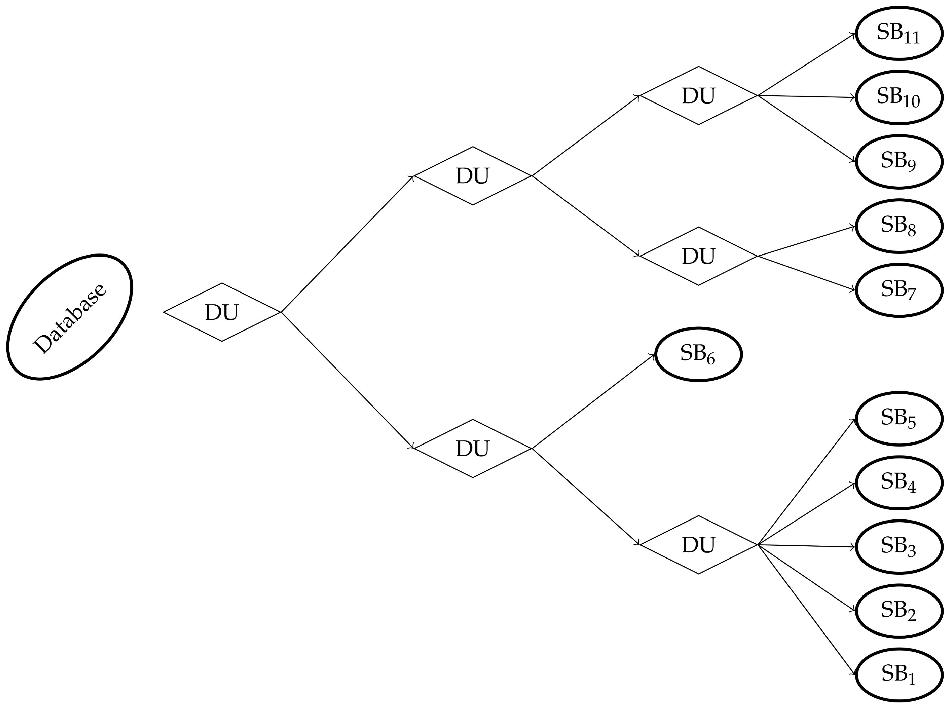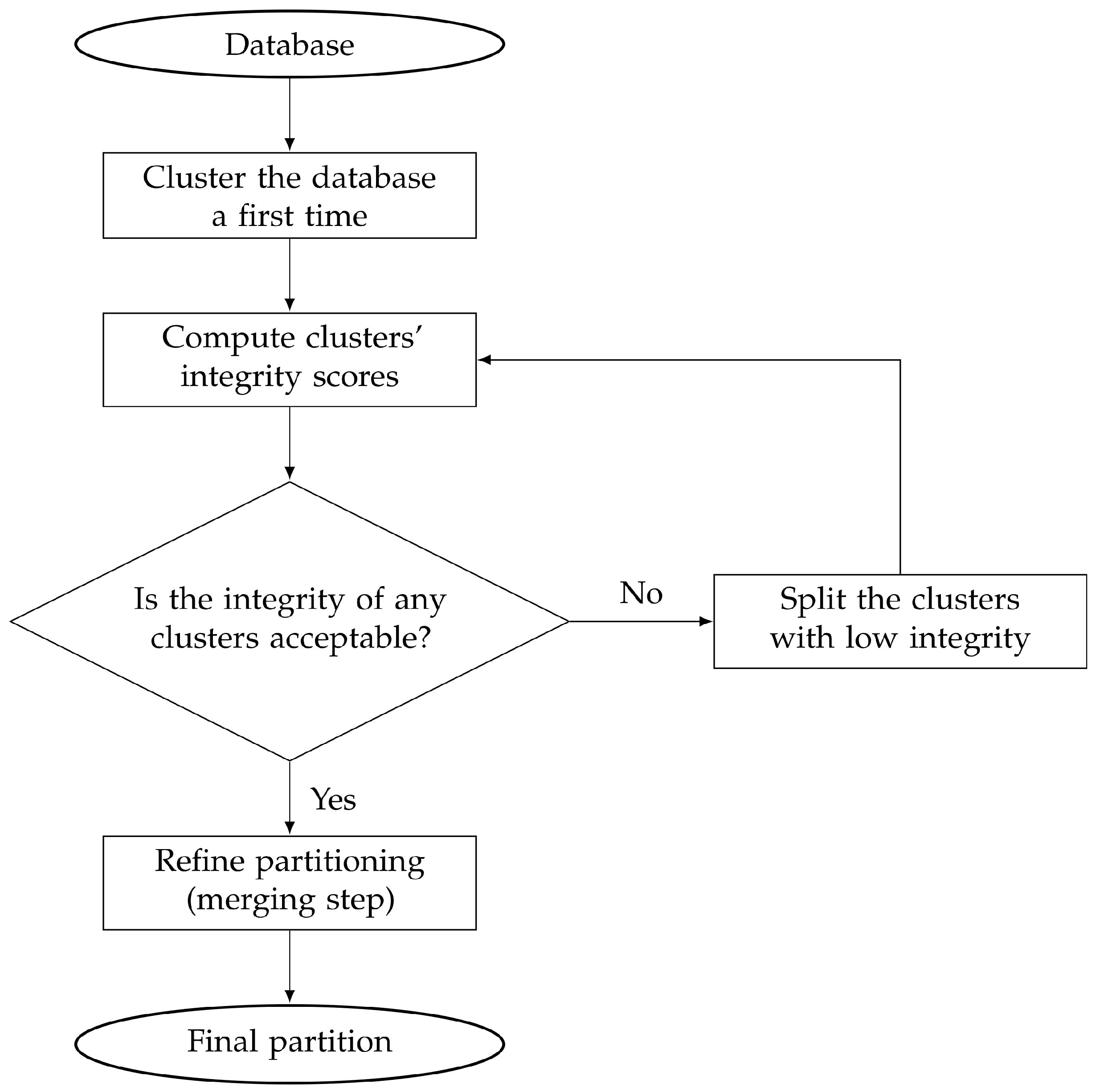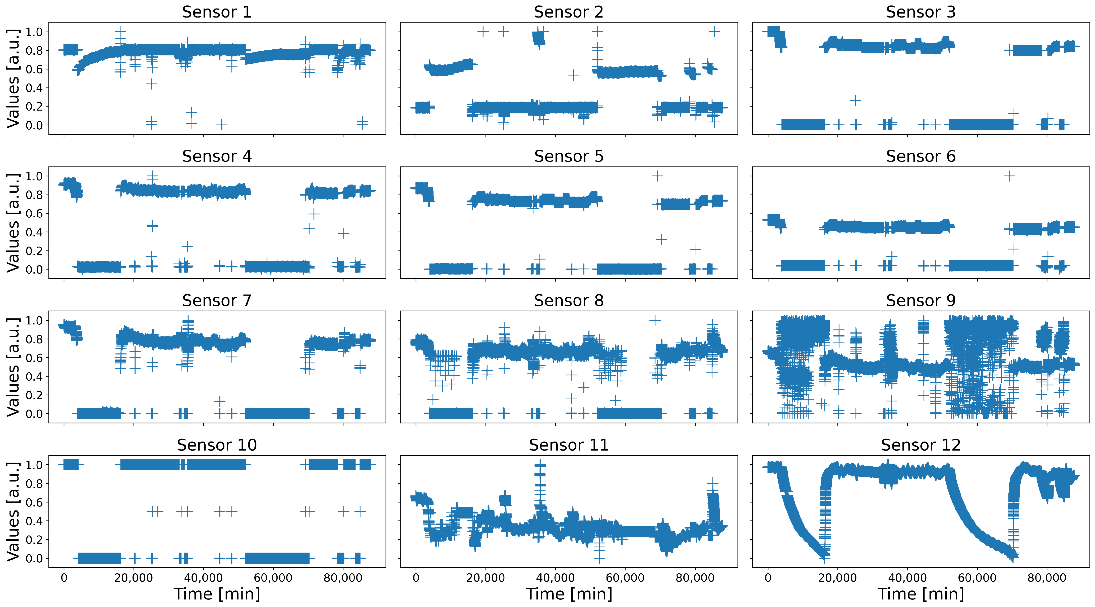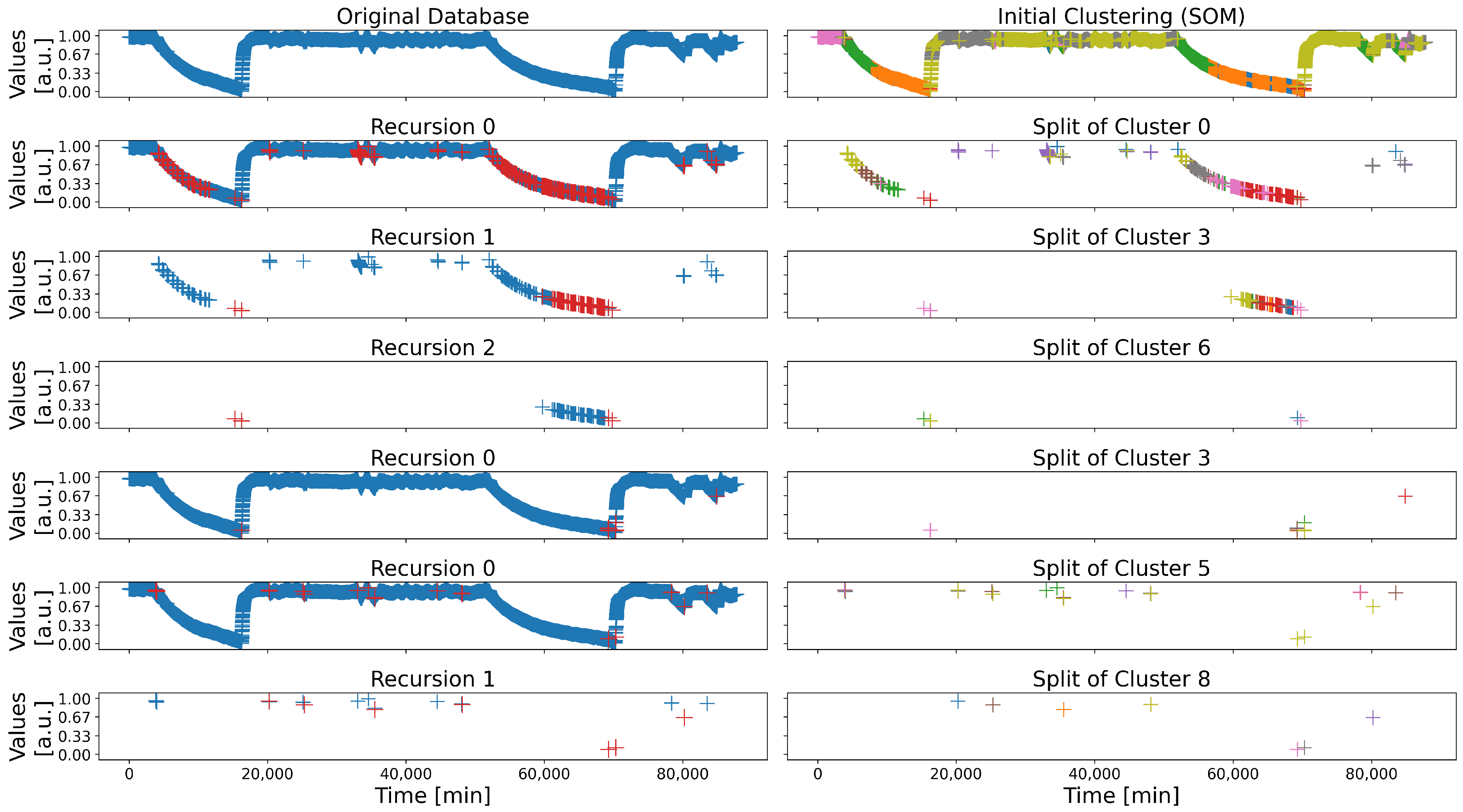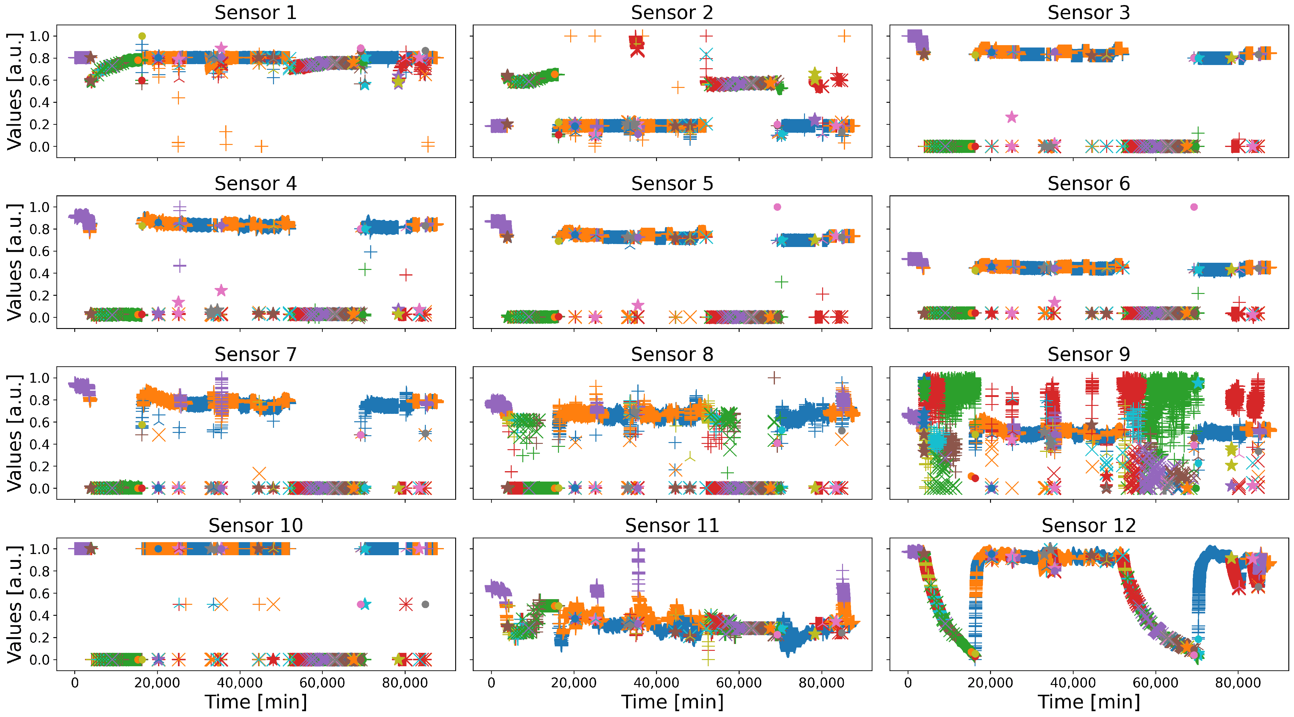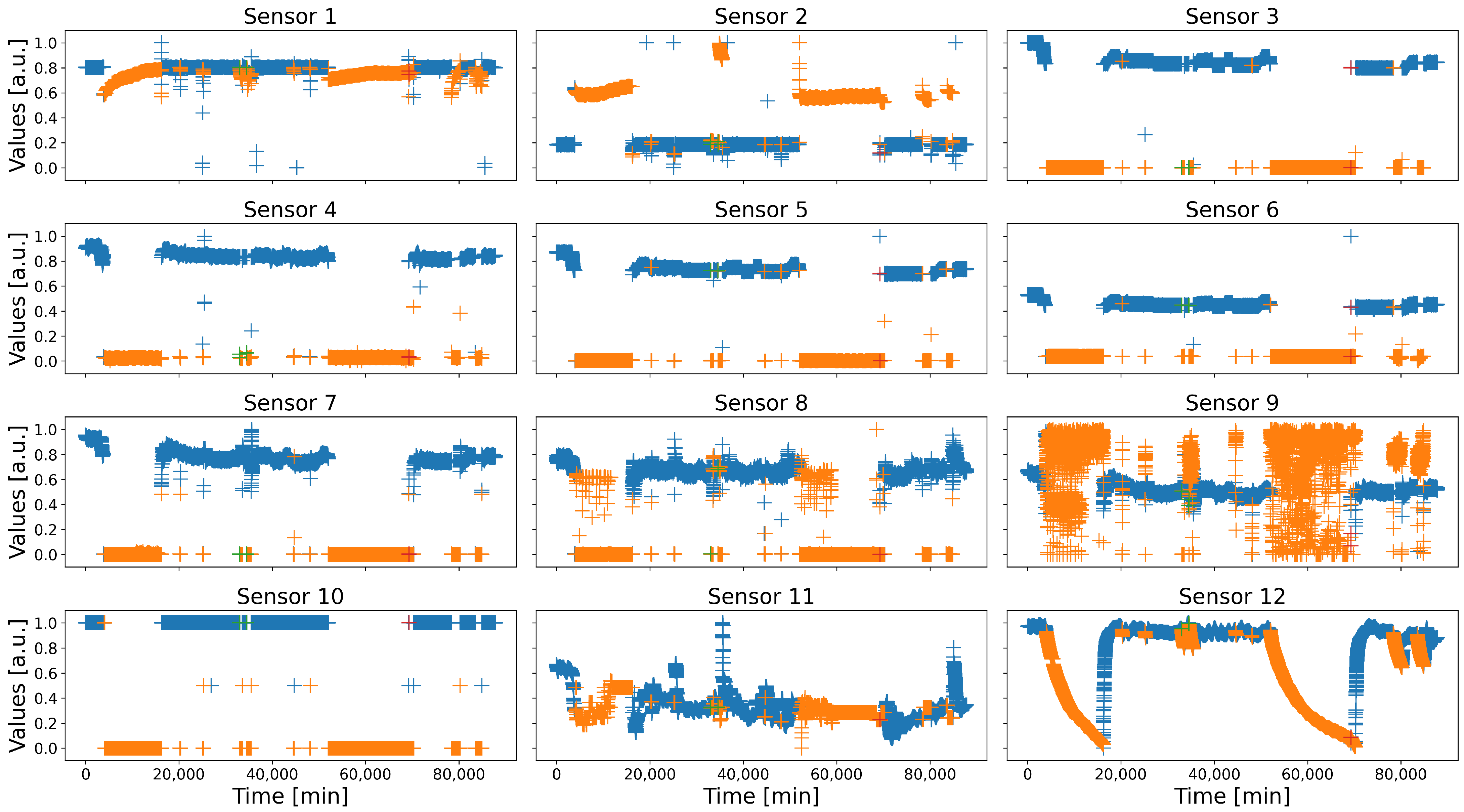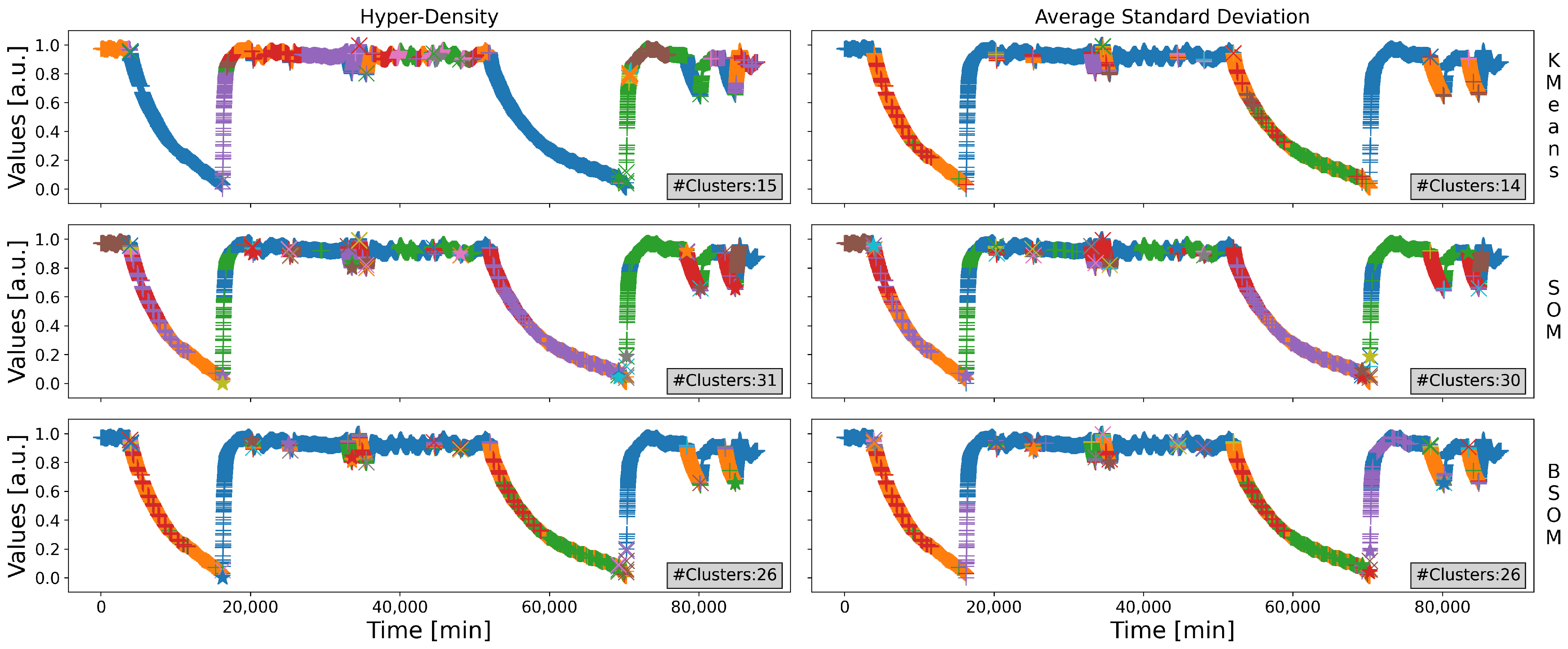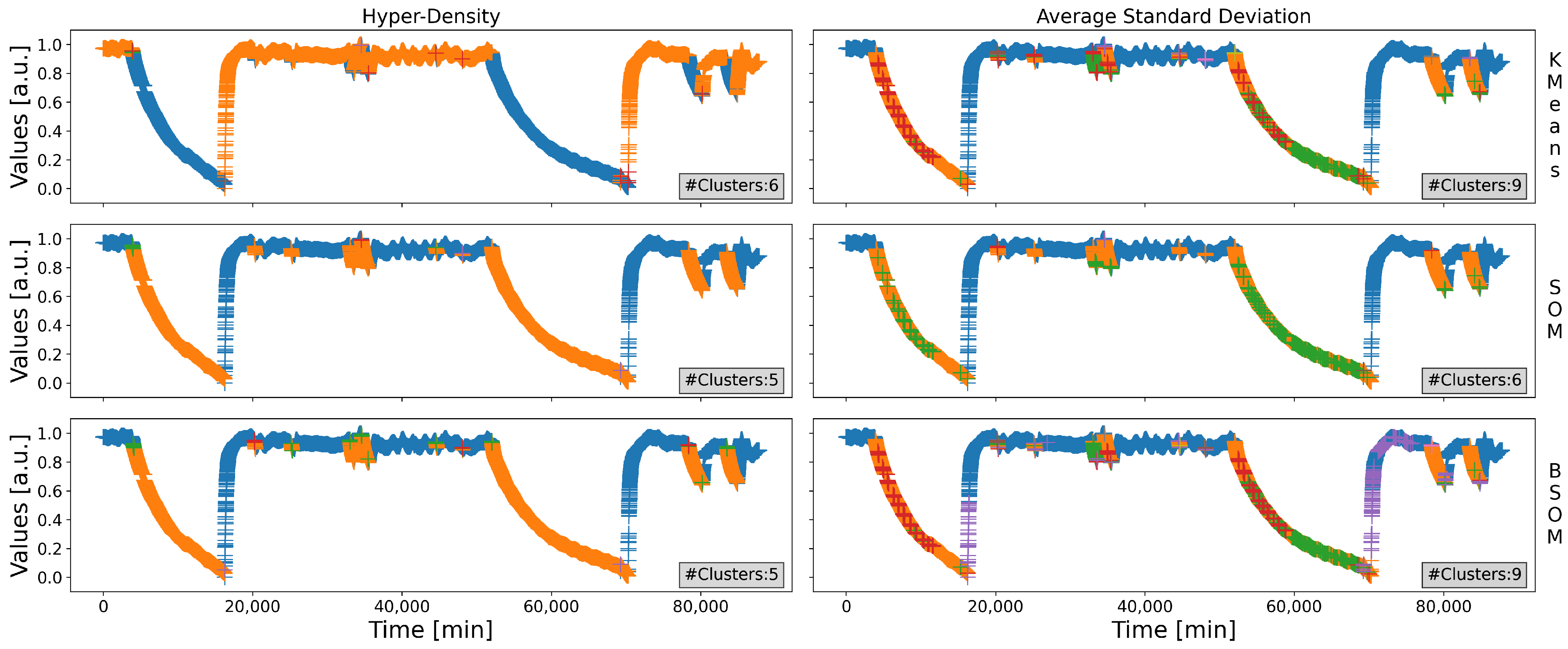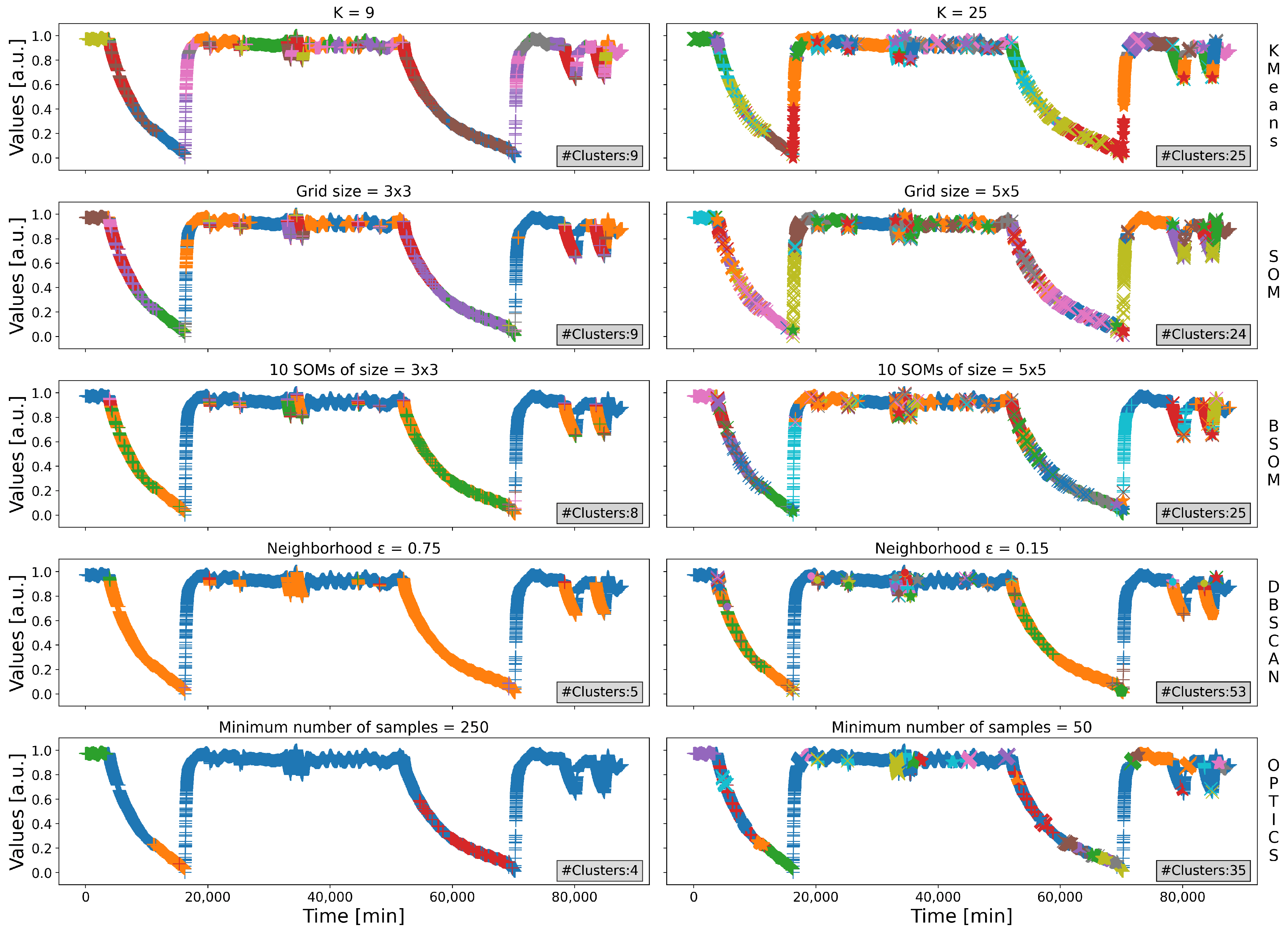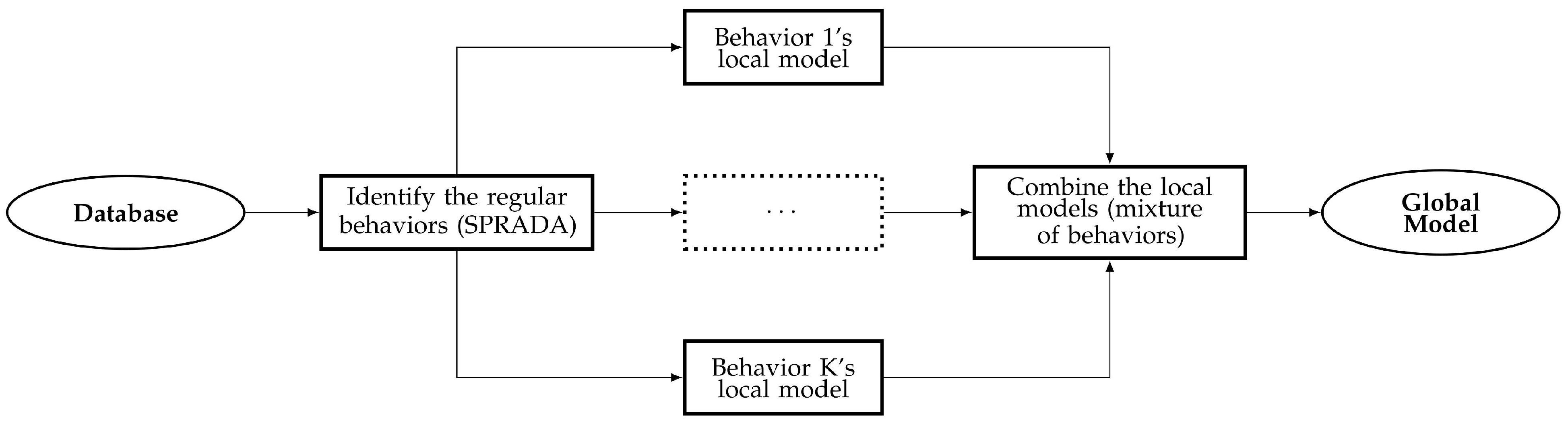For instance, with a high value set for $\epsilon$, the results showed that only the two major states were identified, whilst sub-behaviors (e.g., transient states) were also isolated when using a lower value for $\epsilon$.