
Automated Event Detection and Classification in Soccer: The Potential of Using Multiple Modalities

 , ,
, , 
Abstract
:1. Introduction
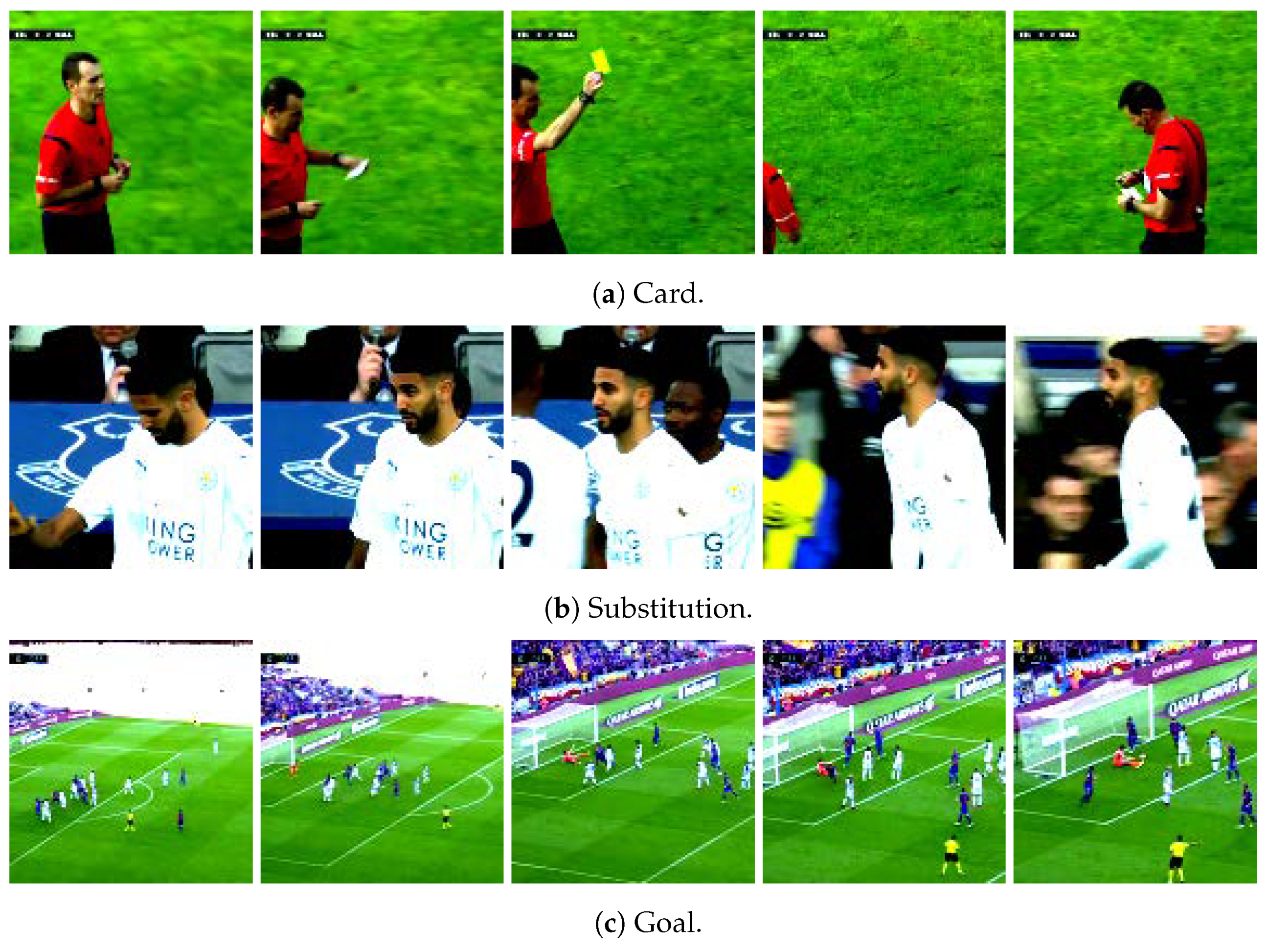
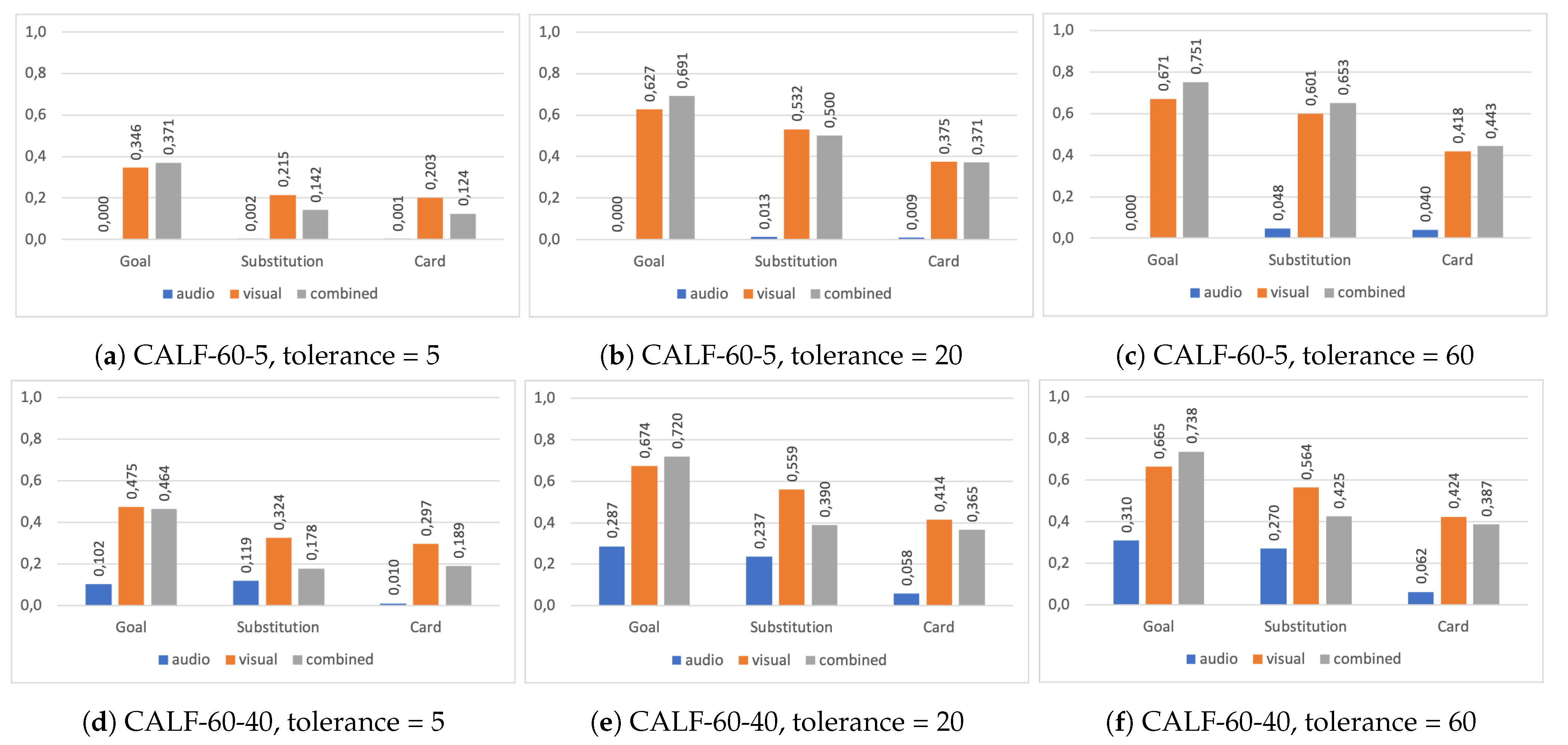
- We implement, configure, and test two state-of-the-art visual models [2,4] built on the ResNet model and assess their detection performance of various soccer events, such as cards, substitutions, and goals, using the SoccerNet dataset [1]. As expected, adding higher tolerance (enabling the models to use more data) improves the performance, trading off event processing delay for event detection (spotting) accuracy.
- We implement a Log-Mel spectrogram-based audio model, testing different audio sample windows and assessing the model’s event detection and classification performance. The results show that using the audio model alone gives poor performance compared to using the visual models.
- We combine the visual and audio models, proving that utilizing all the potential of the data (multiple modalities) improves the performance. We observe a performance increase for various events under different configurations. In particular, for events such as goals, the multimodal approach is superior. For other events such as cards and substitutions, the gain depends more on the tolerances, and in some cases, adding audio information can be detrimental to the performance.
2. Related Work
2.1. Action Detection and Localization
2.2. Event Detection in Soccer Videos
2.3. Multimodality
3. Tested Models
3.1. Visual Model: CALF
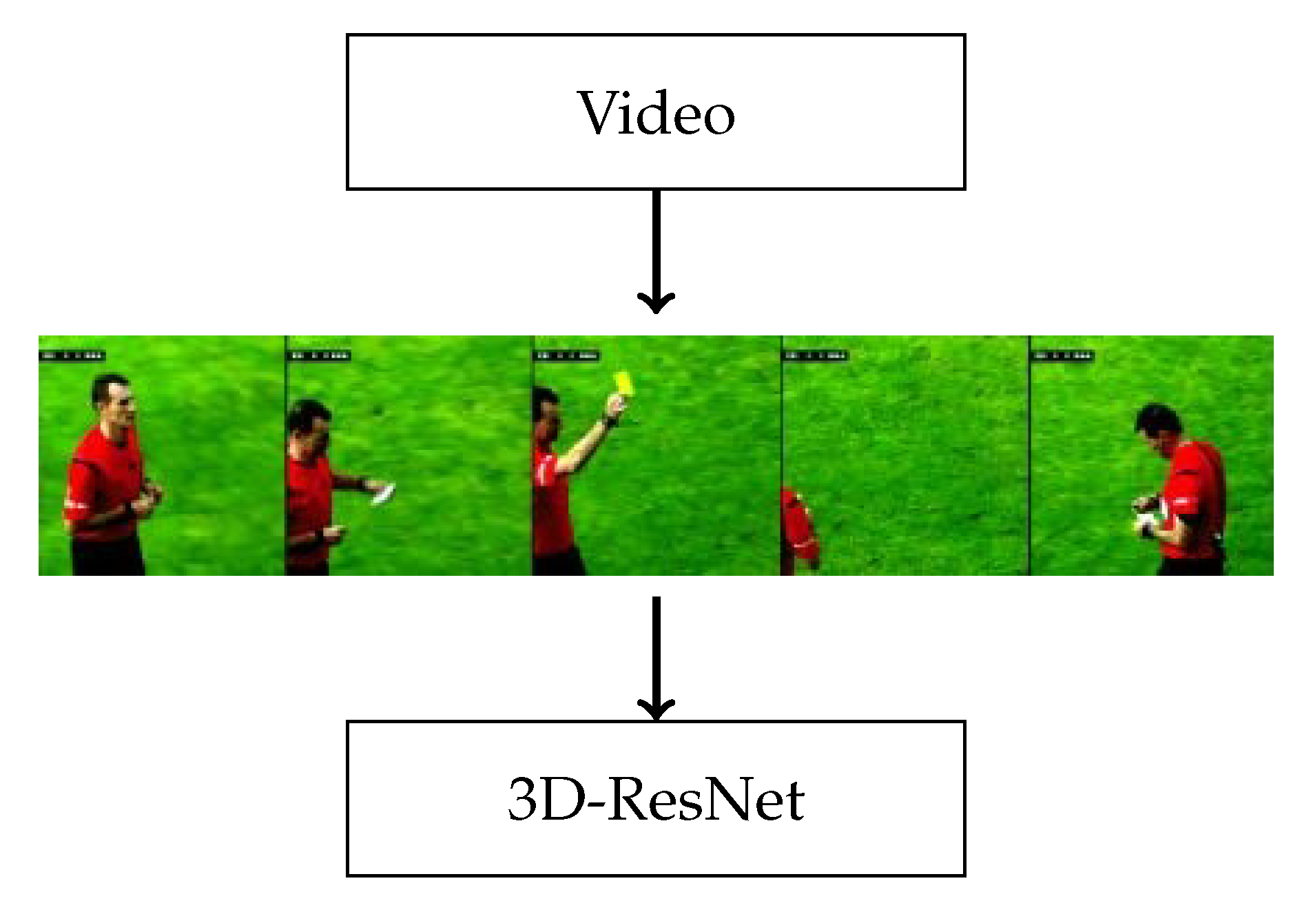
3.2. Visual Model: 3D-CNN
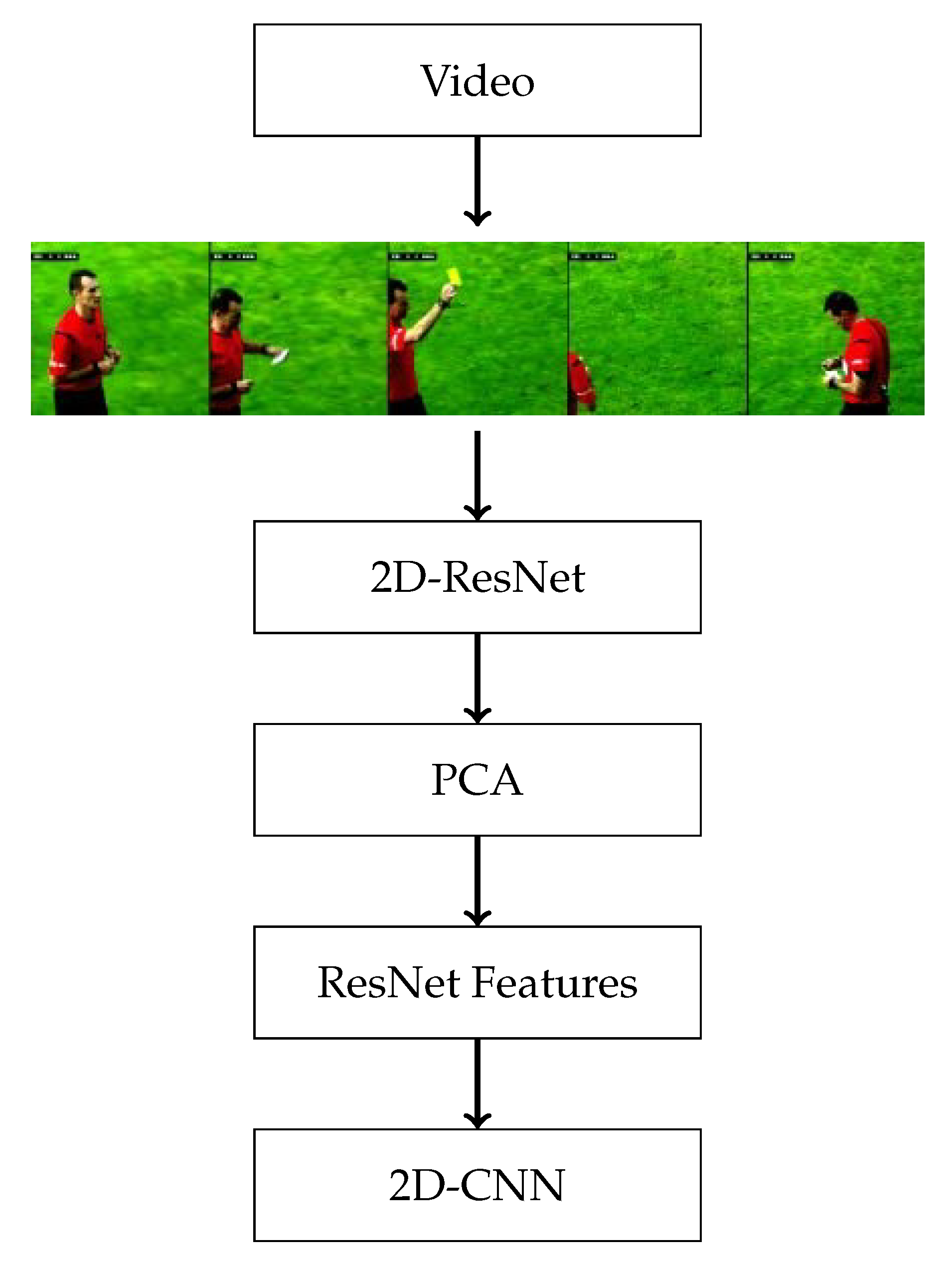
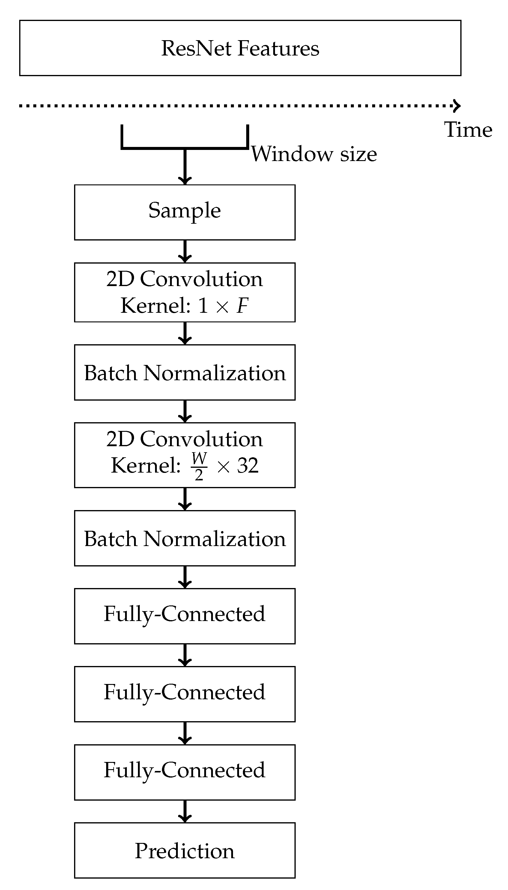
3.3. Visual Model: 2D-CNN
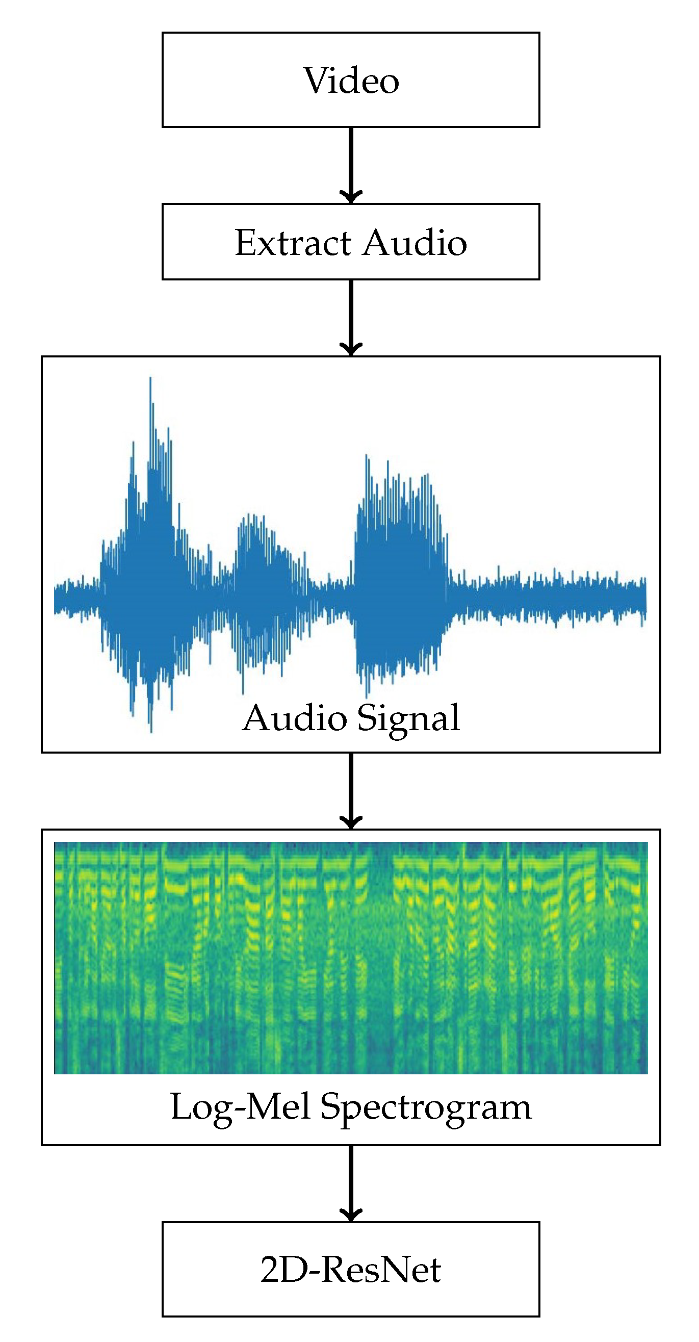
3.4. Audio Model
4. Model Fusion
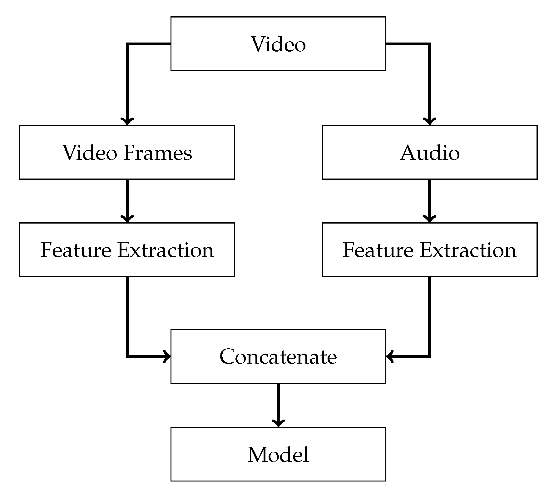
4.1. Early Fusion through Concatenated Features
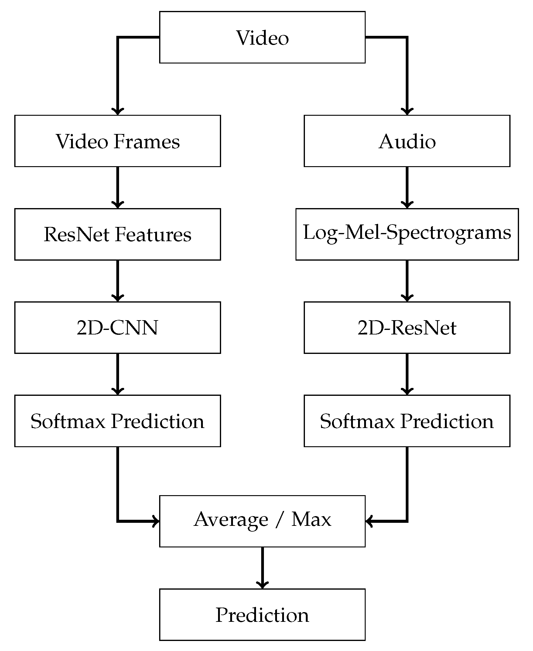
4.2. Late Fusion through Softmax Average and Max
5. Experiments and Results
5.1. Dataset
5.2. Training and Implementation Details
5.2.1. Classification Task
5.2.2. Spotting Task
5.3. Metrics
5.4. Input Window
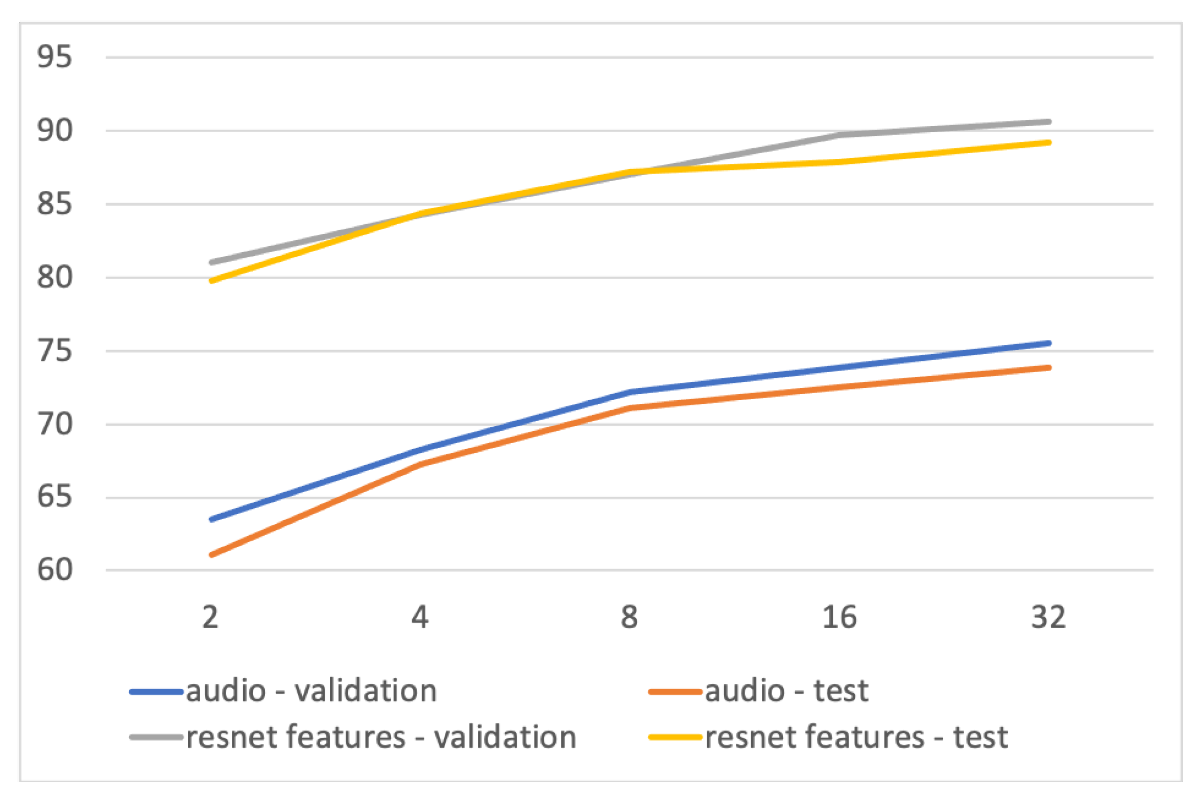
5.4.1. Window Size
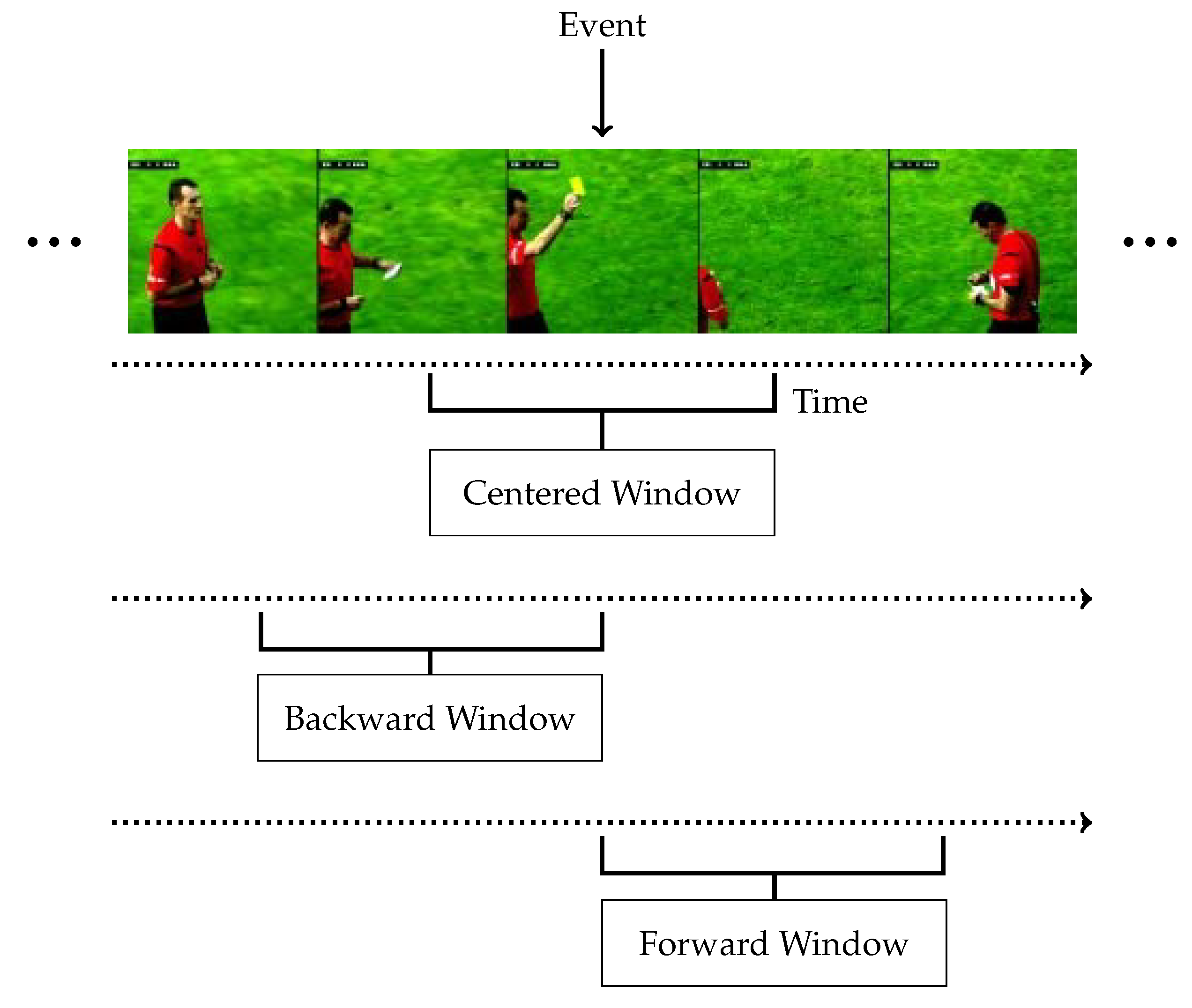
5.4.2. Window Position
- Centered window: A centered window will sample locally around a given event, including both past and future information.
- Backward (shifted) window: For backward window, we only use temporal information up to the point of an event. This can be thought of as a slightly different task, where we predict what is about to occur based on information leading up to an event, rather than what has happened.
- Forward (shifted) window: Samples from just after the event anchor may contain the most relevant information, such as a soccer ball in a goal, with subsequent celebration without ambiguous prior information.
5.5. Classification Performance
5.5.1. Overall Performance
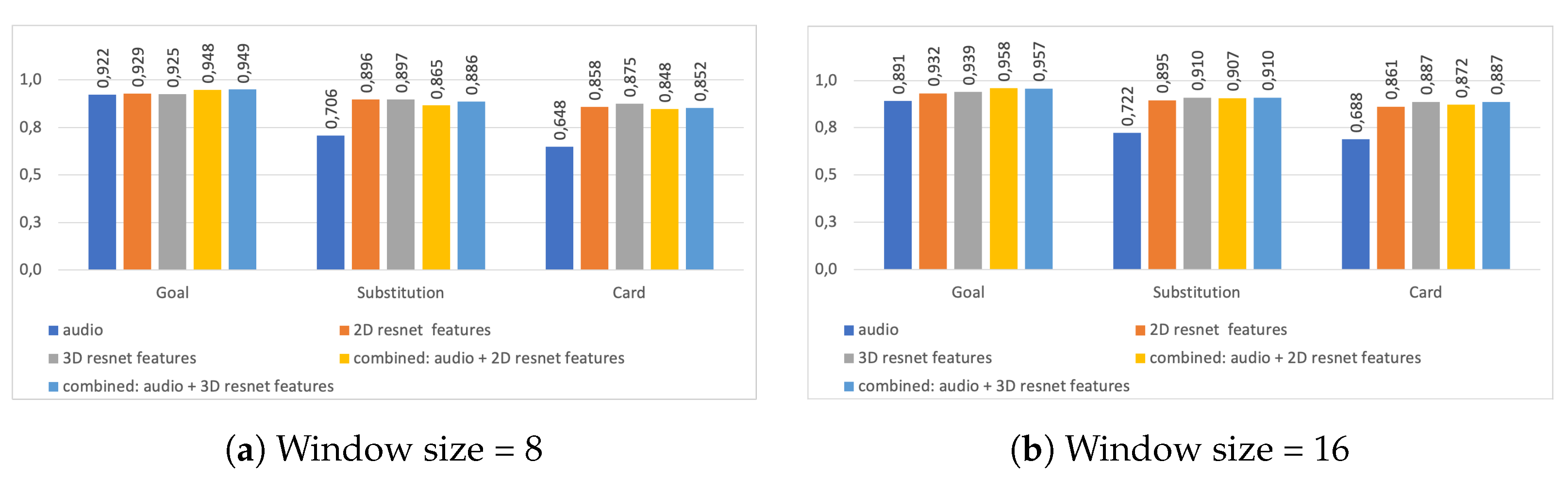
5.5.2. Performance per Event Type
5.6. Spotting Performance
5.6.1. Overall Performance
5.6.2. Performance per Event Type
6. Discussion
7. Summary and Conclusions
Author Contributions
Funding
Institutional Review Board Statement
Informed Consent Statement
Data Availability Statement
Acknowledgments
Conflicts of Interest
References
- Giancola, S.; Amine, M.; Dghaily, T.; Ghanem, B. SoccerNet: A Scalable Dataset for Action Spotting in Soccer Videos. In Proceedings of the Conference on Computer Vision and Pattern Recognition (CVPR) Workshops, Salt Lake City, UT, USA, 18–22 June 2018; pp. 1711–1721. [Google Scholar] [CrossRef] [Green Version]
- Rongved, O.A.N.; Hicks, S.A.; Thambawita, V.; Stensland, H.K.; Zouganeli, E.; Johansen, D.; Riegler, M.A.; Halvorsen, P. Real-Time Detection of Events in Soccer Videos using 3D Convolutional Neural Networks. In Proceedings of the SMEEE International Symposium on Multimedia (ISM), Naples, Italy, 2–4 December 2020; pp. 135–144. [Google Scholar] [CrossRef]
- Rongved, O.A.N.; Hicks, S.A.; Thambawita, V.; Stensland, H.K.; Zouganeli, E.; Johansen, D.; Midoglu, C.; Riegler, M.A.; Halvorsen, P. Using 3D Convolutional Neural Networks for Real-time Detection of Soccer Events. IEEE J. Sel. Top. Signal Process. 2021, 15, 161–187. [Google Scholar] [CrossRef]
- Cioppa, A.; Deliege, A.; Giancola, S.; Ghanem, B.; Droogenbroeck, M.; Gade, R.; Moeslund, T. A Context-Aware Loss Function for Action Spotting in Soccer Videos. In Proceedings of the Conference on Computer Vision and Pattern Recognition (CVPR), Seattle, WA, USA, 13–19 June 2020. [Google Scholar]
- Purwins, H.; Li, B.; Virtanen, T.; Schlüter, J.; Chang, S.; Sainath, T. Deep Learning for Audio Signal Processing. IEEE J. Sel. Top. Signal Process. 2019, 13, 206–219. [Google Scholar] [CrossRef] [Green Version]
- Dalal, N.; Triggs, B.; Schmid, C. Human Detection Using Oriented Histograms of Flow and Appearance. In Proceedings of the ECCV, Graz, Austria, 7–13 May 2006; pp. 428–441. [Google Scholar] [CrossRef] [Green Version]
- Wang, H.; Kläser, A.; Schmid, C.; Liu, C.L. Dense Trajectories and Motion Boundary Descriptors for Action Recognition. Int. J. Comput. Vis. 2013, 103, 60–79. [Google Scholar] [CrossRef] [Green Version]
- Wang, H.; Schmid, C. Action Recognition with Improved Trajectories. In Proceedings of the International Conference on Computer Vision (ICCV), Sydney, Australia, 1–8 December 2013; pp. 3551–3558. [Google Scholar]
- Karpathy, A.; Toderici, G.; Shetty, S.; Leung, T.; Sukthankar, R.; Fei-Fei, L. Large-scale Video Classification with Convolutional Neural Networks. In Proceedings of the International Conference on Computer Vision and Pattern Recognition (CVPR), Columbus, OH, USA, 23–28 June 2014. [Google Scholar]
- Simonyan, K.; Zisserman, A. Two-Stream Convolutional Networks for Action Recognition in Videos. arXiv 2014, arXiv:1406.2199. [Google Scholar]
- Goodale, M.A.; Milner, A.D. Separate visual pathways for perception and action. Trends Neurosci. 1992, 15, 20–25. [Google Scholar] [CrossRef]
- Krizhevsky, A.; Sutskever, I.; Hinton, G.E. ImageNet Classification with Deep Convolutional Neural Networks. In Proceedings of the Annual Conference on Neural Information Processing Systems (NIPS), Lake Tahoe, NV, USA, 3–8 December 2012; pp. 1097–1105. [Google Scholar]
- Deng, J.; Dong, W.; Socher, R.; Li, L.J.; Li, K.; Fei-Fei, L. ImageNet: A Large-Scale Hierarchical Image Database. In Proceedings of the International Conference on Computer Vision and Pattern Recognition (CVPR), Miami, FL, USA, 20–25 June 2009; pp. 248–255. [Google Scholar]
- Tran, D.; Bourdev, L.; Fergus, R.; Torresani, L.; Paluri, M. Learning Spatiotemporal Features with 3D Convolutional Networks. In Proceedings of the ICCV, Santiago, Chile, 7–13 December 2015; pp. 4489–4497. [Google Scholar] [CrossRef] [Green Version]
- Tran, D.; Wang, H.; Torresani, L.; Ray, J.; LeCun, Y.; Paluri, M. A Closer Look at Spatiotemporal Convolutions for Action Recognition. In Proceedings of the International Conference on Computer Vision and Pattern Recognition (CVPR), Salt Lake City, UT, USA, 18–23 June 2018; pp. 6450–6459. [Google Scholar] [CrossRef] [Green Version]
- Feichtenhofer, C.; Fan, H.; Malik, J.; He, K. SlowFast Networks for Video Recognition. In Proceedings of the International Conference on Computer Vision (ICCV), Seoul, Korea, 27 October–2 November 2019; pp. 6202–6211. [Google Scholar]
- Carreira, J.; Zisserman, A. Quo Vadis, Action Recognition? A New Model and the Kinetics Dataset. arXiv 2018, arXiv:1705.07750. [Google Scholar]
- Szegedy, C.; Liu, W.; Jia, Y.; Sermanet, P.; Reed, S.; Anguelov, D.; Erhan, D.; Vanhoucke, V.; Rabinovich, A. Going Deeper with Convolutions. In Proceedings of the Conference on Computer Vision and Pattern Recognition (CVPR), Boston, MA, USA, 7–12 June 2015; pp. 1–9. [Google Scholar]
- Feichtenhofer, C.; Pinz, A.; Zisserman, A. Convolutional Two-Stream Network Fusion for Video Action Recognition. In Proceedings of the International Conference on Computer Vision and Pattern Recognition (CVPR), Las Vegas, NV, USA, 27–30 June 2016; pp. 1933–1941. [Google Scholar] [CrossRef] [Green Version]
- Feichtenhofer, C.; Pinz, A.; Wildes, R.P. Spatiotemporal Residual Networks for Video Action Recognition. In Proceedings of the Annual Conference on Neural Information Processing Systems (NIPS), Barcelona, Spain, 5–10 December 2016; pp. 3476–3484. [Google Scholar]
- He, K.; Zhang, X.; Ren, S.; Sun, J. Deep Residual Learning for Image Recognition. In Proceedings of the International Conference on Computer Vision and Pattern Recognition (CVPR), Las Vegas, NV, USA, 27–30 June 2016; pp. 770–778. [Google Scholar]
- Wang, L.; Qiao, Y.; Tang, X. Action Recognition with Trajectory-Pooled Deep-Convolutional Descriptors. In Proceedings of the International Conference on Computer Vision and Pattern Recognition (CVPR), Boston, MA, USA, 7–12 June 2015; pp. 4305–4314. [Google Scholar] [CrossRef] [Green Version]
- Shou, Z.; Wang, D.; Chang, S.F. Temporal Action Localization in Untrimmed Videos via Multi-stage CNNs. In Proceedings of the International Conference on Computer Vision and Pattern Recognition (CVPR), Las Vegas, NV, USA, 27–30 June 2016; pp. 1049–1058. [Google Scholar] [CrossRef] [Green Version]
- Wang, L.; Xiong, Y.; Wang, Z.; Qiao, Y.; Lin, D.; Tang, X.; Van Gool, L. Temporal Segment Networks: Towards Good Practices for Deep Action Recognition. In Proceedings of the ECCV, Amsterdam, The Netherlands, 11–14 October 2016; pp. 20–36. [Google Scholar]
- Donahue, J.; Hendricks, L.A.; Rohrbach, M.; Venugopalan, S.; Guadarrama, S.; Saenko, K.; Darrell, T. Long-term Recurrent Convolutional Networks for Visual Recognition and Description. In Proceedings of the IEEE Conference on Computer Vision and Pattern Recognition (CVPR), Boston, MA, USA, 7–12 June 2015. [Google Scholar]
- Soomro, K.; Zamir, A.R.; Shah, M. UCF101: A Dataset of 101 Human Actions Classes From Videos in The Wild. arXiv 2012, arXiv:1212.0402. [Google Scholar]
- Qiu, Z.; Yao, T.; Ngo, C.W.; Tian, X.; Mei, T. Learning Spatio-Temporal Representation with Local and Global Diffusion. arXiv 2019, arXiv:1906.05571. [Google Scholar]
- Kalfaoglu, M.E.; Kalkan, S.; Alatan, A.A. Late Temporal Modeling in 3D CNN Architectures with BERT for Action Recognition. arXiv 2020, arXiv:2008.01232. [Google Scholar]
- Kuehne, H.; Jhuang, H.; Garrote, E.; Poggio, T.; Serre, T. HMDB51: A Large Video Database for Human Motion Recognition. In Proceedings of the International Conference on Computer Vision (ICCV), Barcelona, Spain, 13–16 November 2011; pp. 2556–2563. [Google Scholar] [CrossRef] [Green Version]
- Singh, G.; Cuzzolin, F. Untrimmed Video Classification for Activity Detection: Submission to ActivityNet Challenge. arXiv 2016, arXiv:1607.01979. [Google Scholar]
- Zhao, Y.; Xiong, Y.; Wang, L.; Wu, Z.; Tang, X.; Lin, D. Temporal Action Detection with Structured Segment Networks. arXiv 2017, arXiv:1704.06228. [Google Scholar]
- Chao, Y.W.; Vijayanarasimhan, S.; Seybold, B.; Ross, D.A.; Deng, J.; Sukthankar, R. Rethinking the Faster R-CNN Architecture for Temporal Action Localization. arXiv 2018, arXiv:1804.07667. [Google Scholar]
- Lin, T.; Zhao, X.; Shou, Z. Single Shot Temporal Action Detection. In Proceedings of the ACM MM, Mountain View, CA, USA, 23–27 October 2017. [Google Scholar] [CrossRef] [Green Version]
- Buch, S.; Escorcia, V.; Ghanem, B.; Fei-Fei, L.; Niebles, J.C. End-to-End, Single-Stream Temporal Action Detection in Untrimmed Videos. In Proceedings of the BMVC, London, UK, 4–7 September 2017. [Google Scholar]
- Idrees, H.; Zamir, A.R.; Jiang, Y.; Gorban, A.; Laptev, I.; Sukthankar, R.; Shah, M. The THUMOS challenge on action recognition for videos “in the wild”. Comput. Vis. Image Underst. 2017, 155, 1–23. [Google Scholar] [CrossRef] [Green Version]
- Lin, T.; Liu, X.; Li, X.; Ding, E.; Wen, S. BMN: Boundary-Matching Network for Temporal Action Proposal Generation. In Proceedings of the International Conference on Computer Vision (ICCV), Seoul, Korea, 27 October–2 November 2019. [Google Scholar]
- Lin, T.; Zhao, X.; Su, H.; Wang, C.; Yang, M. BSN: Boundary Sensitive Network for Temporal Action Proposal Generation. In Proceedings of the ECCV, Munich, Germany, 8–14 September 2018. [Google Scholar]
- Ren, S.; He, K.; Girshick, R.; Sun, J. Faster R-CNN: Towards Real-Time Object Detection with Region Proposal Networks. In Proceedings of the Advances in Neural Information Processing Systems (NIPS), Montreal, QC, Canada, 7–12 December 2015; pp. 91–99. [Google Scholar]
- Xu, H.; Das, A.; Saenko, K. R-C3D: Region Convolutional 3D Network for Temporal Activity Detection. In Proceedings of the International Conference on Computer Vision (ICCV), Venice, Italy, 22–29 October 2017. [Google Scholar]
- Buch, S.; Escorcia, V.; Shen, C.; Ghanem, B.; Niebles, J.C. SST: Single-Stream Temporal Action Proposals. In Proceedings of the International Conference on Computer Vision and Pattern Recognition (CVPR), Honolulu, HI, USA, 21–26 July 2017; pp. 6373–6382. [Google Scholar]
- Heilbron, F.; Niebles, J.C.; Ghanem, B. Fast Temporal Activity Proposals for Efficient Detection of Human Actions in Untrimmed Videos. In Proceedings of the CVPR, Las Vegas, NV, USA, 27–30 June 2016. [Google Scholar] [CrossRef]
- Spagnolo, P.; Leo, M.; Mazzeo, P.L.; Nitti, M.; Stella, E.; Distante, A. Non-invasive Soccer Goal Line Technology: A Real Case Study. In Proceedings of the International Conference on Computer Vision and Pattern Recognition (CVPR) Workshops, Portland, OR, USA, 23–28 June 2013; pp. 1011–1018. [Google Scholar] [CrossRef]
- Mazzeo, P.L.; Spagnolo, P.; Leo, M.; D’Orazio, T. Visual Players Detection and Tracking in Soccer Matches. In Proceedings of the IEEE International Conference on Advanced Video and Signal Based Surveillance (AVSS), Santa Fe, NM, USA, 1–3 September 2008; pp. 326–333. [Google Scholar] [CrossRef]
- Stensland, H.K.; Gaddam, V.R.; Tennøe, M.; Helgedagsrud, E.; Næss, M.; Alstad, H.K.; Mortensen, A.; Langseth, R.; Ljødal, S.; Landsverk, O.; et al. Bagadus: An Integrated Real-Time System for Soccer Analytics. ACM Trans. Multimed. Comput. Commun. Appl. 2014, 10, 1–21. [Google Scholar] [CrossRef]
- Thamaraimanalan, T.; Naveena, D.; Ramya, M.; Madhubala, M. Prediction and Classification of Fouls in Soccer Game using Deep Learning. Ir. Interdiscip. J. Sci. Res. 2020, 4, 66–78. [Google Scholar]
- Gaddam, V.R.; Eg, R.; Langseth, R.; Griwodz, C.; Halvorsen, P. The Cameraman Operating My Virtual Camera is Artificial: Can the Machine Be as Good as a Human? ACM Trans. Multimed. Comput. Commun. Appl. 2015, 11, 1–20. [Google Scholar] [CrossRef]
- Johansen, D.; Johansen, H.; Aarflot, T.; Hurley, J.; Kvalnes, R.; Gurrin, C.; Zav, S.; Olstad, B.; Aaberg, E.; Endestad, T.; et al. DAVVI: A Prototype for the next Generation Multimedia Entertainment Platform. In Proceedings of the International Conference on Multimedia (ACM MM), Vancouver, BC, Canada, 19–24 October 2009; pp. 989–990. [Google Scholar] [CrossRef]
- Wang, J.; Xu, C.; Chng, E.; Tian, Q. Sports highlight detection from keyword sequences using HMM. In Proceedings of the IEEE International Conference on Multimedia Expo (ICME), Taipei, Taiwan, 27–30 June 2004; Volume 1, pp. 599–602. [Google Scholar] [CrossRef]
- Dhanuja, S.P.; Waykar, S.B. A Survey on Event Recognition and Summarization in Football Videos. Int. J. Sci. Res. 2014, 3, 2365–2367. [Google Scholar]
- Xiong, Z.; Radhakrishnan, R.; Divakaran, A.; Huang, T. Audio events detection based highlights extraction from baseball, golf and soccer games in a unified framework. In Proceedings of the International Conference on Multimedia and Expo (ICME), Baltimore, MD, USA, 6–9 July 2003; Volume 3, p. III-401. [Google Scholar] [CrossRef]
- Pixi, Z.; Hongyan, L.; Wei, W. Research on Event Detection of Soccer Video Based on Hidden Markov Model. In Proceedings of the 2010 International Conference on Computational and Information Sciences, Chengdu, China, 17–19 December 2010; pp. 865–868. [Google Scholar] [CrossRef]
- Qian, X.; Liu, G.; Wang, H.; Li, Z.; Wang, Z. Soccer Video Event Detection by Fusing Middle Level Visual Semantics of an Event Clip. In Proceedings of the Advances in Multimedia Information Processing (PCM), Shanghai, China, 21–24 September 2010; Springer: Berlin/Heidelberg, Germany, 2010; pp. 439–451. [Google Scholar]
- Qian, X.; Wang, H.; Liu, G. HMM based soccer video event detection using enhanced mid-level semantic. Multimed. Tools Appl. 2012, 60, 233–255. [Google Scholar] [CrossRef]
- Itoh, H.; Takiguchi, T.; Ariki, Y. Event Detection and Recognition Using HMM with Whistle Sounds. In Proceedings of the 2013 International Conference on Signal-Image Technology Internet-Based Systems, Kyoto, Japan, 2–5 December 2013; pp. 14–21. [Google Scholar] [CrossRef]
- Xu, M.; Maddage, N.; Xu, C.; Kankanhalli, M.; Tian, Q. Creating audio keywords for event detection in soccer video. In Proceedings of the International Conference on Multimedia and Expo (ICME), Baltimore, MD, USA, 6–9 July 2003; Volume 2, p. II-281. [Google Scholar] [CrossRef] [Green Version]
- Ye, Q.; Huang, Q.; Gao, W.; Jiang, S. Exciting Event Detection in Broadcast Soccer Video with Mid-Level Description and Incremental Learning. In Proceedings of the ACM International Conference on Multimedia (MM), Singapore, 6–11 November 2005; pp. 455–458. [Google Scholar] [CrossRef]
- Sadlier, D.; O’Connor, N. Event detection in field sports video using audio-visual features and a support vector machine. IEEE Trans. Circuits Syst. Video Technol. 2005, 15, 1225–1233. [Google Scholar] [CrossRef] [Green Version]
- Jain, N.; Chaudhury, S.; Roy, S.D.; Mukherjee, P.; Seal, K.; Talluri, K. A Novel Learning-Based Framework for Detecting Interesting Events in Soccer Videos. In Proceedings of the Indian Conference on Computer Vision, Graphics Image Processing, Bhubaneswar, India, 16–19 December 2008; pp. 119–125. [Google Scholar] [CrossRef]
- Zawbaa, H.M.; El-Bendary, N.; Hassanien, A.E.; Abraham, A. SVM-based soccer video summarization system. In Proceedings of the the World Congress on Nature and Biologically Inspired Computing, Salamanca, Spain, 19–21 October 2011; pp. 7–11. [Google Scholar] [CrossRef] [Green Version]
- Fakhar, B.; Kanan, H.; Behrad, A. Event detection in soccer videos using unsupervised learning of Spatio-temporal features based on pooled spatial pyramid model. Multimed. Tools Appl. 2019, 78, 16995–17025. [Google Scholar] [CrossRef]
- Jiang, H.; Lu, Y.; Xue, J. Automatic Soccer Video Event Detection Based on a Deep Neural Network Combined CNN and RNN. In Proceedings of the IEEE International Conference on Tools with Artificial Intelligence (ICTAI), San Jose, CA, USA, 6–8 November 2016; pp. 490–494. [Google Scholar] [CrossRef]
- Tang, K.; Bao, Y.; Zhao, Z.; Zhu, L.; Lin, Y.; Peng, Y. AutoHighlight: Automatic Highlights Detection and Segmentation in Soccer Matches. In Proceedings of the IEEE International Conference on Big Data (Big Data), Seattle, WA, USA, 10–13 December 2018; pp. 4619–4624. [Google Scholar] [CrossRef]
- Khan, A.; Lazzerini, B.; Calabrese, G.; Serafini, L. Soccer Event Detecion. In Proceedings of the the International Conference on Image Processing and Pattern Recognition (IPPR), Copenhagen, Denmark, 28–29 April 2018. [Google Scholar] [CrossRef]
- Hong, Y.; Ling, C.; Ye, Z. End-to-end soccer video scene and event classification with deep transfer learning. In Proceedings of the International Conference on Intelligent Systems and Computer Vision (ISCV), Fez, Morocco, 2–4 April 2018; pp. 1–4. [Google Scholar] [CrossRef]
- Yu, J.; Lei, A.; Hu, Y. Soccer Video Event Detection Based on Deep Learning. In Proceedings of the MultiMedia Modeling (MMM), Thessaloniki, Greece, 8–11 January 2019; pp. 377–389. [Google Scholar]
- Kay, W.; Carreira, J.; Simonyan, K.; Zhang, B.; Hillier, C.; Vijayanarasimhan, S.; Viola, F.; Green, T.; Back, T.; Natsev, P.; et al. The Kinetics Human Action Video Dataset. arXiv 2017, arXiv:1705.06950. [Google Scholar]
- Redmon, J.; Divvala, S.; Girshick, R.; Farhadi, A. You Only Look Once: Unified, Real-Time Object Detection. arXiv 2016, arXiv:1506.02640. [Google Scholar]
- Vats, K.; Fani, M.; Walters, P.; Clausi, D.A.; Zelek, J. Event detection in coarsely annotated sports videos via parallel multi receptive field 1D convolutions. arXiv 2020, arXiv:2004.06172. [Google Scholar]
- Zhou, X.; Kang, L.; Cheng, Z.; He, B.; Xin, J. Feature Combination Meets Attention: Baidu Soccer Embeddings and Transformer based Temporal Detection. arXiv 2021, arXiv:2106.14447. [Google Scholar]
- Sadlier, D.A.; O’Connor, N.; Marlow, S.; Murphy, N. A combined audio-visual contribution to event detection in field sports broadcast video. In Case study: Gaelic football. In Proceedings of the IEEE International Symposium on Signal Processing and Information Technology (ISSPIT), Darmstadt, Germany, 17 December 2003; pp. 552–555. [Google Scholar] [CrossRef] [Green Version]
- Ortega, J.; Senoussaoui, M.; Granger, E.; Pedersoli, M.; Cardinal, P.; Koerich, A. Multimodal Fusion with Deep Neural Networks for Audio-Video Emotion Recognition. arXiv 2019, arXiv:1907.03196. [Google Scholar]
- Xiao, F.; Lee, Y.J.; Grauman, K.; Malik, J.; Feichtenhofer, C. Audiovisual SlowFast Networks for Video Recognition. arXiv 2020, arXiv:2001.08740. [Google Scholar]
- Vanderplaetse, B.; Dupont, S. Improved Soccer Action Spotting Using Both Audio and Video Streams. In Proceedings of the International Conference on Computer Vision and Pattern Recognition (CVPR) Workshops, Seattle, WA, USA, 14–19 June 2020. [Google Scholar]
- Gao, X.; Liu, X.; Yang, T.; Deng, G.; Peng, H.; Zhang, Q.; Li, H.; Liu, J. Automatic Key Moment Extraction and Highlights Generation Based on Comprehensive Soccer Video Understanding. In Proceedings of the IEEE International Conference on Multimedia Expo Workshops (ICMEW), London, UK, 6–10 July 2020; pp. 1–6. [Google Scholar] [CrossRef]
- Wang, X.; Girshick, R.; Gupta, A.; He, K. Non-Local Neural Networks. In Proceedings of the Conference on Computer Vision and Pattern Recognition (CVPR), Salt Lake City, UT, USA, 13–18 June 2018. [Google Scholar]
- Zolfaghari, M.; Singh, K.; Brox, T. ECO: Efficient Convolutional Network for Online Video Understanding. In Proceedings of the European Conference on Computer Vision (ECCV), Munich, Germany, 8–14 September 2018. [Google Scholar]
- Khaleghi, B.; Khamis, A.; Karray, F.O.; Razavi, S.N. Multisensor Data Fusion: A Review of the State-of-the-Art. Inf. Fusion 2013, 14, 28–44. [Google Scholar] [CrossRef]
- Paszke, A.; Gross, S.; Massa, F.; Lerer, A.; Bradbury, J.; Chanan, G.; Killeen, T.; Lin, Z.; Gimelshein, N.; Antiga, L.; et al. PyTorch: An Imperative Style, High-Performance Deep Learning Library. In Proceedings of the Annual Conference on Neural Information Processing Systems (NIPS), Vancouver, QC, Canada, 8–14 December 2019; pp. 8024–8035. [Google Scholar]
- Islam, M.R.; Paul, M.; Antolovich, M.; Kabir, A. Sports Highlights Generation using Decomposed Audio Information. In Proceedings of the IEEE International Conference on Multimedia Expo Workshops (ICMEW), Shanghai, China, 8–12 July 2019; pp. 579–584. [Google Scholar] [CrossRef]
- Deliège, A.; Cioppa, A.; Giancola, S.; Seikavandi, M.J.; Dueholm, J.V.; Nasrollahi, K.; Ghanem, B.; Moeslund, T.B.; Droogenbroeck, M.V. SoccerNet-v2: A Dataset and Benchmarks for Holistic Understanding of Broadcast Soccer Videos. arXiv 2021, arXiv:2011.13367. [Google Scholar]


| Class | Training | Validation | Test |
|---|---|---|---|
| Card | 1296 | 396 | 453 |
| Substitution | 1708 | 562 | 579 |
| Goal | 961 | 356 | 326 |
| Background | 1855 | 636 | 653 |
| Total | 5820 | 1950 | 2011 |
| Data Type | ||||
|---|---|---|---|---|
| Task | Model(s) | ResNet features | Video | Audio |
| Classification | 2D-CNN | ✓ | ||
| 3D-CNN | ✓ | |||
| Audio | ✓ | |||
| 2D-CNN + audio | ✓ | ✓ | ||
| 3D-CNN + audio | ✓ | ✓ | ||
| Spotting | CALF | ✓ | ||
| Audio | ✓ | |||
| CALF + audio | ✓ | ✓ | ||
| Accuracy (%) | ||||
|---|---|---|---|---|
| Model-Dataset | Window Size | Centered Window | Backward Window | Forward Window |
| Audio-validation | 16 | 75.23 | 66.82 | 70.62 |
| Audio-test | 16 | 75.09 | 65.09 | 69.02 |
| ResNet-validation | 16 | 89.33 | 76.62 | 89.08 |
| ResNet-test | 16 | 88.12 | 75.98 | 89.01 |
| Accuracy (%) | |||||
|---|---|---|---|---|---|
| Dataset | Window Size | Audio | Video | Softmax Average | Softmax Max |
| Validation | 8 | 71.11 | 88.31 | 87.71 | 87.17 |
| 16 | 72.55 | 89.90 | 89.06 | 88.81 | |
| Test | 8 | 72.15 | 89.69 | 88.35 | 87,89 |
| 16 | 73.90 | 90.87 | 89.07 | 88.92 | |
| Accuracy (%) | ||||||
|---|---|---|---|---|---|---|
| Dataset | Window Size | Audio | ResNet | Concat. | Softmax Average | Softmax Max |
| Validation | 2 | 63.54 | 81.08 | 84.46 | 78.72 | 78.46 |
| 4 | 68.26 | 84.26 | 87.64 | 82.31 | 82.31 | |
| 8 | 72.15 | 87.08 | 88.51 | 86.21 | 85.79 | |
| 16 | 73.90 | 89.74 | 91.23 | 89.38 | 89.03 | |
| 32 | 75.49 | 90.67 | 92.51 | 92.05 | 91.59 | |
| Test | 2 | 61.11 | 79.81 | 77.27 | 76.93 | 76.08 |
| 4 | 67.28 | 84.3 | 81.15 | 82.40 | 81.85 | |
| 8 | 71.11 | 87.22 | 80.91 | 85.98 | 85.83 | |
| 16 | 72.55 | 87.87 | 82.15 | 89.21 | 88.91 | |
| 32 | 73.89 | 89.21 | 87.02 | 90.85 | 90.65 | |
| W = 8 | W = 16 | ||||||
|---|---|---|---|---|---|---|---|
| Class | Input Type | Precision | Recall | F1 | Precision | Recall | F1 |
| Card | Audio | 0.650 | 0.647 | 0.648 | 0.672 | 0.704 | 0.688 |
| Card | Video | 0.876 | 0.874 | 0.875 | 0.900 | 0.874 | 0.887 |
| Card | Video + audio | 0.844 | 0.861 | 0.852 | 0.868 | 0.868 | 0.868 |
| Substitution | Audio | 0.694 | 0.718 | 0.706 | 0.777 | 0.674 | 0.722 |
| Substitution | Video | 0.925 | 0.870 | 0.897 | 0.949 | 0.874 | 0.910 |
| Substitution | Video + audio | 0.894 | 0.877 | 0.886 | 0.944 | 0.877 | 0.910 |
| Goal | Audio | 0.942 | 0.902 | 0.922 | 0.908 | 0.874 | 0.891 |
| Goal | Video | 0.924 | 0.926 | 0.925 | 0.913 | 0.966 | 0.939 |
| Goal | Video + audio | 0.954 | 0.945 | 0.949 | 0.954 | 0.960 | 0.957 |
| Background | Audio | 0.658 | 0.654 | 0.656 | 0.646 | 0.712 | 0.677 |
| Background | Video | 0.836 | 0.879 | 0.857 | 0.853 | 0.905 | 0.878 |
| Background | Video + audio | 0.848 | 0.855 | 0.851 | 0.834 | 0.884 | 0.858 |
| W = 2 | W = 4 | W = 8 | W = 16 | W = 32 | ||||||||||||
|---|---|---|---|---|---|---|---|---|---|---|---|---|---|---|---|---|
| Class | Input type | Precision | Recall | F1 | Precision | Recall | F1 | Precision | Recall | F1 | Precision | Recall | F1 | Precision | Recall | F1 |
| Card | Audio | 0.564 | 0.552 | 0.558 | 0.601 | 0.618 | 0.609 | 0.650 | 0.647 | 0.648 | 0.672 | 0.704 | 0.688 | 0.632 | 0.664 | 0.648 |
| Card | ResNet | 0.811 | 0.757 | 0.783 | 0.836 | 0.808 | 0.822 | 0.869 | 0.848 | 0.858 | 0.873 | 0.850 | 0.861 | 0.873 | 0.892 | 0.882 |
| Card | Combined | 0.776 | 0.751 | 0.763 | 0.796 | 0.790 | 0.793 | 0.865 | 0.832 | 0.848 | 0.870 | 0.874 | 0.872 | 0.867 | 0.892 | 0.879 |
| Substitution | Audio | 0.625 | 0.573 | 0.598 | 0.651 | 0.672 | 0.661 | 0.694 | 0.718 | 0.706 | 0.777 | 0.674 | 0.722 | 0.817 | 0.770 | 0.793 |
| Substitution | ResNet | 0.866 | 0.794 | 0.829 | 0.885 | 0.874 | 0.879 | 0.909 | 0.883 | 0.896 | 0.923 | 0.869 | 0.895 | 0.933 | 0.870 | 0.901 |
| Substitution | Combined | 0.803 | 0.741 | 0.771 | 0.818 | 0.841 | 0.830 | 0.857 | 0.872 | 0.865 | 0.922 | 0.893 | 0.907 | 0.945 | 0.914 | 0.929 |
| Goal | Audio | 0.851 | 0.825 | 0.838 | 0.919 | 0.902 | 0.910 | 0.942 | 0.902 | 0.922 | 0.908 | 0.874 | 0.891 | 0.867 | 0.837 | 0.852 |
| Goal | ResNet | 0.803 | 0.936 | 0.864 | 0.885 | 0.923 | 0.904 | 0.898 | 0.942 | 0.919 | 0.941 | 0.923 | 0.932 | 0.959 | 0.942 | 0.950 |
| Goal | Combined | 0.878 | 0.929 | 0.903 | 0.937 | 0.951 | 0.944 | 0.940 | 0.957 | 0.948 | 0.969 | 0.948 | 0.958 | 0.960 | 0.948 | 0.954 |
| Background | Audio | 0.524 | 0.579 | 0.550 | 0.622 | 0.597 | 0.609 | 0.658 | 0.654 | 0.656 | 0.646 | 0.712 | 0.677 | 0.691 | 0.714 | 0.702 |
| Background | ResNet | 0.734 | 0.761 | 0.747 | 0.793 | 0.802 | 0.798 | 0.830 | 0.845 | 0.838 | 0.820 | 0.885 | 0.851 | 0.842 | 0.887 | 0.864 |
| Background | Combined | 0.684 | 0.727 | 0.705 | 0.791 | 0.769 | 0.780 | 0.818 | 0.819 | 0.819 | 0.846 | 0.876 | 0.861 | 0.882 | 0.896 | 0.889 |
| Tolerance = 5 | Tolerance = 20 | Tolerance = 40 | Tolerance = 60 | |||||||||||
|---|---|---|---|---|---|---|---|---|---|---|---|---|---|---|
| Model | Input type | Precision | Recall | mAP | Precision | Recall | mAP | Precision | Recall | mAP | Precision | Recall | mAP | Average-mAP |
| CALF-60-5 | Audio | NaN | 0.0735 | 0.0010 | NaN | 0.1913 | 0.0075 | NaN | 0.3721 | 0.0187 | NaN | 0.3501 | 0.0293 | 0.0145 |
| CALF-60-5 | ResNet | 0.1551 | 0.2947 | 0.2545 | 0.4385 | 0.5507 | 0.5113 | 0.5488 | 0.6110 | 0.5495 | 0.5766 | 0.6147 | 0.5634 | 0.5092 |
| CALF-60-5 | Combined | 0.1425 | 0.1729 | 0.2123 | 0.4330 | 0.4780 | 0.5209 | 0.5453 | 0.5547 | 0.5998 | 0.5889 | 0.6135 | 0.6156 | 0.5408 |
| CALF-60-20 | Audio | 0.0695 | 0.0704 | 0.0771 | 0.2416 | 0.1505 | 0.1940 | 0.3146 | 0.2084 | 0.2321 | 0.3729 | 0.2117 | 0.2475 | 0.2069 |
| CALF-60-20 | ResNet | 0.3259 | 0.3069 | 0.3655 | 0.6401 | 0.5117 | 0.5493 | 0.6882 | 0.5327 | 0.5871 | 0.6145 | 0.5790 | 0.5971 | 0.5574 |
| CALF-60-20 | Combined | 0.2419 | 0.2303 | 0.2769 | 0.5290 | 0.4659 | 0.4915 | 0.5984 | 0.5016 | 0.5683 | 0.6176 | 0.5398 | 0.6136 | 0.5231 |
| CALF-120-40 | Audio | NaN | 0.0374 | 0.0007 | NaN | 0.1519 | 0.0045 | NaN | 0.1585 | 0.0161 | NaN | 0.2454 | 0.0264 | 0.0123 |
| CALF-120-40 | ResNet | 0.2195 | 0.2535 | 0.2869 | 0.6383 | 0.5819 | 0.6067 | 0.7199 | 0.6438 | 0.6425 | 0.7446 | 0.6506 | 0.6530 | 0.6007 |
| CALF-120-40 | Combined | 0.1681 | 0.1855 | 0.2139 | 0.5749 | 0.4674 | 0.5579 | 0.6254 | 0.5836 | 0.6106 | 0.6602 | 0.5931 | 0.6345 | 0.5629 |
| Tolerance = 5 | Tolerance = 20 | Tolerance = 40 | Tolerance = 60 | ||||||||||||
|---|---|---|---|---|---|---|---|---|---|---|---|---|---|---|---|
| Model | Class | Input type | Precision | Recall | AP | Precision | Recall | AP | Precision | Recall | AP | Precision | Recall | AP | Average-AP |
| CALF-60-5 | Card | Audio | 0.0030 | 0.0667 | 0.0009 | 0.0096 | 0.2133 | 0.0089 | 0.0197 | 0.4378 | 0.0239 | 0.0254 | 0.5644 | 0.0398 | 0.0183 |
| CALF-60-5 | Card | ResNet | 0.1271 | 0.2733 | 0.2031 | 0.3489 | 0.4978 | 0.3748 | 0.4348 | 0.5556 | 0.4067 | 0.4486 | 0.5622 | 0.4184 | 0.3701 |
| CALF-60-5 | Card | Combined | 0.1455 | 0.0689 | 0.1242 | 0.4673 | 0.2222 | 0.3716 | 0.5779 | 0.2556 | 0.4218 | 0.6109 | 0.3000 | 0.4427 | 0.3728 |
| CALF-60-5 | Substitution | Audio | 0.0022 | 0.1537 | 0.0021 | 0.0102 | 0.3604 | 0.0134 | 0.0192 | 0.6784 | 0.0320 | 0.0275 | 0.4859 | 0.0479 | 0.0254 |
| CALF-60-5 | Substitution | ResNet | 0.1464 | 0.2827 | 0.2148 | 0.4353 | 0.5530 | 0.5323 | 0.5668 | 0.6148 | 0.5868 | 0.6185 | 0.6131 | 0.6007 | 0.5213 |
| CALF-60-5 | Substitution | Combined | 0.0941 | 0.2014 | 0.1421 | 0.2912 | 0.5583 | 0.5003 | 0.4183 | 0.6784 | 0.6311 | 0.4732 | 0.7491 | 0.6528 | 0.5299 |
| CALF-60-5 | Goal | Audio | NaN | 0 | 0 | NaN | 0 | 0 | NaN | 0 | 0 | NaN | 0 | 0 | 0 |
| CALF-60-5 | Goal | ResNet | 0.1918 | 0.3282 | 0.3456 | 0.5312 | 0.6012 | 0.6269 | 0.6448 | 0.6626 | 0.6551 | 0.6626 | 0.6687 | 0.6709 | 0.6111 |
| CALF-60-5 | Goal | Combined | 0.1879 | 0.2485 | 0.3705 | 0.5406 | 0.6534 | 0.6909 | 0.6398 | 0.7301 | 0.7465 | 0.6825 | 0.7914 | 0.7514 | 0.6879 |
| CALF-60-20 | Card | Audio | 0.0229 | 0.0178 | 0.0101 | 0.0609 | 0.0156 | 0.0580 | 0.0879 | 0.0356 | 0.0761 | 0.1069 | 0.0311 | 0.0885 | 0.0618 |
| CALF-60-20 | Card | ResNet | 0.2574 | 0.2511 | 0.2973 | 0.5012 | 0.4511 | 0.4144 | 0.5293 | 0.4622 | 0.4495 | 0.4395 | 0.5089 | 0.4670 | 0.4238 |
| CALF-60-20 | Card | Combined | 0.2243 | 0.1889 | 0.1891 | 0.4330 | 0.3444 | 0.3647 | 0.5044 | 0.3800 | 0.4391 | 0.5221 | 0.4200 | 0.4676 | 0.3865 |
| CALF-60-20 | Substitution | Audio | 0.0251 | 0.1413 | 0.1193 | 0.1104 | 0.3410 | 0.2367 | 0.1623 | 0.4576 | 0.3111 | 0.2194 | 0.4753 | 0.3439 | 0.2695 |
| CALF-60-20 | Substitution | ResNet | 0.2832 | 0.2862 | 0.3244 | 0.6297 | 0.5318 | 0.5594 | 0.7048 | 0.5654 | 0.6177 | 0.6161 | 0.6237 | 0.6231 | 0.5640 |
| CALF-60-20 | Substitution | Combined | 0.1063 | 0.2014 | 0.1779 | 0.3040 | 0.5318 | 0.3896 | 0.3974 | 0.5848 | 0.4708 | 0.4320 | 0.6290 | 0.5550 | 0.4250 |
| CALF-60-20 | Goal | Audio | 0.1604 | 0.0521 | 0.1019 | 0.5536 | 0.0951 | 0.2872 | 0.6935 | 0.1319 | 0.3090 | 0.7925 | 0.1288 | 0.3101 | 0.2782 |
| CALF-60-20 | Goal | ResNet | 0.4371 | 0.3834 | 0.4746 | 0.7895 | 0.5521 | 0.6741 | 0.8304 | 0.5706 | 0.6941 | 0.7880 | 0.6043 | 0.7012 | 0.6653 |
| CALF-60-20 | Goal | Combined | 0.3952 | 0.3006 | 0.4637 | 0.8500 | 0.5215 | 0.7201 | 0.8934 | 0.5399 | 0.7951 | 0.8986 | 0.5706 | 0.8182 | 0.7383 |
| CALF-120-40 | Card | Audio | 0.0015 | 0.0222 | 0.0004 | 0.0068 | 0.1022 | 0.0042 | 0.0155 | 0.2333 | 0.0184 | 0.0261 | 0.3933 | 0.0343 | 0.0140 |
| CALF-120-40 | Card | ResNet | 0.2103 | 0.2444 | 0.2394 | 0.5624 | 0.5311 | 0.4802 | 0.6268 | 0.5822 | 0.5239 | 0.6522 | 0.6000 | 0.5399 | 0.4775 |
| CALF-120-40 | Card | Combined | 0.1505 | 0.1378 | 0.1587 | 0.5236 | 0.2956 | 0.4043 | 0.5230 | 0.4044 | 0.4453 | 0.5503 | 0.4133 | 0.4607 | 0.4012 |
| CALF-120-40 | Substitution | Audio | 0.0038 | 0.0901 | 0.0017 | 0.0099 | 0.3534 | 0.0091 | 0.0203 | 0.2420 | 0.0299 | 0.0287 | 0.3428 | 0.0449 | 0.0231 |
| CALF-120-40 | Substitution | ResNet | 0.1745 | 0.2155 | 0.2341 | 0.5685 | 0.5795 | 0.6269 | 0.6933 | 0.6590 | 0.6660 | 0.7218 | 0.6555 | 0.6735 | 0.6006 |
| CALF-120-40 | Substitution | Combined | 0.1047 | 0.1979 | 0.1562 | 0.3844 | 0.5053 | 0.5102 | 0.4682 | 0.6378 | 0.5629 | 0.5384 | 0.6572 | 0.5988 | 0.5021 |
| CALF-120-40 | Goal | Audio | NaN | 0 | 0 | NaN | 0 | 0 | NaN | 0 | 0 | NaN | 0 | 0 | 0 |
| CALF-120-40 | Goal | ResNet | 0.2737 | 0.3006 | 0.3872 | 0.7841 | 0.6350 | 0.7131 | 0.8396 | 0.6902 | 0.7375 | 0.8598 | 0.6963 | 0.7455 | 0.6912 |
| CALF-120-40 | Goal | Combined | 0.2491 | 0.2209 | 0.3269 | 0.8167 | 0.6012 | 0.7592 | 0.8851 | 0.7086 | 0.8237 | 0.8919 | 0.7086 | 0.8441 | 0.7507 |
Publisher’s Note: MDPI stays neutral with regard to jurisdictional claims in published maps and institutional affiliations. |
© 2021 by the authors. Licensee MDPI, Basel, Switzerland. This article is an open access article distributed under the terms and conditions of the Creative Commons Attribution (CC BY) license (https://creativecommons.org/licenses/by/4.0/).
Share and Cite
Nergård Rongved, O.A.; Stige, M.; Hicks, S.A.; Thambawita, V.L.; Midoglu, C.; Zouganeli, E.; Johansen, D.; Riegler, M.A.; Halvorsen, P. Automated Event Detection and Classification in Soccer: The Potential of Using Multiple Modalities. Mach. Learn. Knowl. Extr. 2021, 3, 1030-1054. https://doi.org/10.3390/make3040051
Nergård Rongved OA, Stige M, Hicks SA, Thambawita VL, Midoglu C, Zouganeli E, Johansen D, Riegler MA, Halvorsen P. Automated Event Detection and Classification in Soccer: The Potential of Using Multiple Modalities. Machine Learning and Knowledge Extraction. 2021; 3(4):1030-1054. https://doi.org/10.3390/make3040051
Chicago/Turabian StyleNergård Rongved, Olav Andre, Markus Stige, Steven Alexander Hicks, Vajira Lasantha Thambawita, Cise Midoglu, Evi Zouganeli, Dag Johansen, Michael Alexander Riegler, and Pål Halvorsen. 2021. "Automated Event Detection and Classification in Soccer: The Potential of Using Multiple Modalities" Machine Learning and Knowledge Extraction 3, no. 4: 1030-1054. https://doi.org/10.3390/make3040051