Applying a Neural Network-Based Machine Learning to Laser-Welded Spark Plasma Sintered Steel: Predicting Vickers Micro-Hardness

Abstract

This paper presents an artificial neural network (ANN) approach to the estimation of the Vickers hardness parameter at the weld zone of laser-welded sintered duplex stainless steel. The sintered welded stainless-steel hardness is primarily determined by the sintering conditions and laser welding processing parameters. In the current investigation, the process parameters for both the sintering and welding processes were trained by ANNs machine learning (ML) model using a TensorFlow framework for the microhardness predictions of laser-welded sintered duplex stainless steel (DSS 2507 grade). A neural network is trained using a thorough dataset. The mean absolute error (MAE), mean square error (MSE), root mean square error (RMSE), and R² for the train and test data were calculated. The predicted values were in good agreement with the measured hardness values. Based on the results obtained, the ANN method can be effectively used to predict the mechanical properties of materials.

1. Introduction

The past few decades have witnessed an increase in dual-phase stainless steel steels (DSS). DSS has found applications in oil, gas, chemical industries, and pressure vessels, where a combination of outstanding corrosion resistance and high mechanical strength are major requirements [1]. Powder metallurgy (PM) can effectively control the microstructure of bulk samples, or metallic alloys [2]. In addition, the PM manufacturing doubles as the most cost-effective method, compared to other manufacturing processes, such as casting and forging, in terms of producing complex profile geometries. Meanwhile, it is necessary to join PM parts to other materials produced by other manufacturing processes [3]. 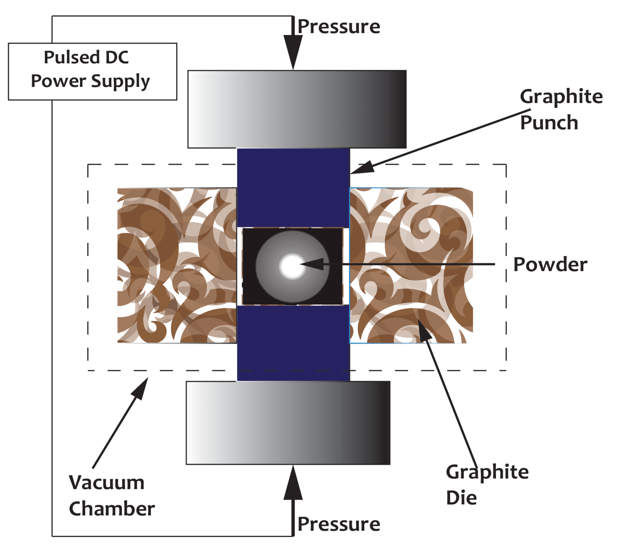Therefore, it is required to understand joining or welding PM parts together [4]. Looking through the different PM manufacturing processes, spark plasma sintering (SPS) has been outstanding; it produces a material with fine microstructures and uniform dispersion of reinforcing particles. Additionally, improved hardness and strength can be achieved, among other amazing attributes. Reducing the sintering time that results in low energy consumption [5,6,7,8].

In the material processing industry, it is pertinent for materials to undergo precise and consistent output to meet the required quality standard set. Therefore, a neural network has recently been employed as a technique developed for processing the elements, named neurons, that have connections with each other [9]. Given adequate data and algorithms, machine learning, with the help of a computer, can determine all known physical laws without the involvement of humans. Therefore, the machine learning method learns the rules that govern datasets by working with part of the data and automatically creates a model to provide a prediction.

An artificial neural network (ANN) is fashioned against the brain’s mode of operation. There are usually three layers in the ANN algorithm: input, hidden, and output. The hidden layer neuron receives signals from other neurons, integrates the imputs and compute final results [10]. A neural network that has one hidden layer (or ≤ 2 hidden layers) is usually known as a multi-layer perceptron or shallow neural network (SNN), usually trained by a back-propagation (BP) algorithm. It has, however, seen diverse applications in materials science, such as predicting materials properties [11,12,13,14,15,16,17,18,19,20,21].

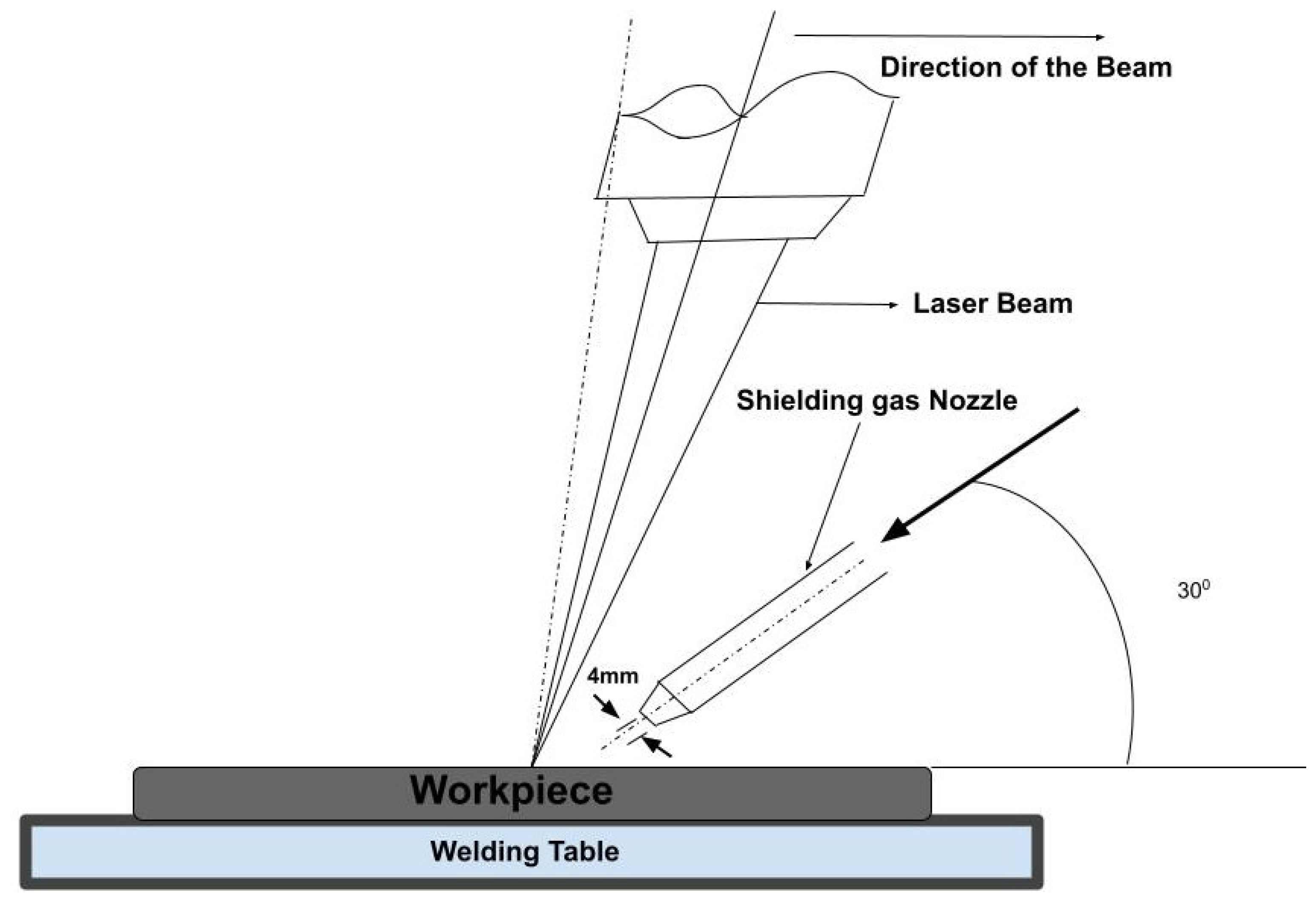
Dehabadi et al. [22] studied the application of ANN to predict the micro-hardness of friction-welded AA6061 sheets. The study showed that the value for mean absolute percentage error (MAPE) in training activity for both ANNs was less than 4.83%. Eventually, the results of their work showed acceptable deviance for the actual microhardness. Balasubramanian et al. [9] also evaluated the ability of neural networks in predicting and analyzing the effect of input parameters, viz., welding speed, beam power, and beam angle on the depth of penetration and bead width, which comprises the output parameters for a laser beam-welded stainless steel. In the end, their work showed the proper abilities of neural networks to predict the parameters for butt laser welding. The mechanical properties of welded steel X70 pipeline were predicted using the neural network modeling by Adel et al. [23]. The input parameter for the predictions was based on the chemical compositions of the alloy. Absolution fraction variance and relative error were used as the metrics to determine the prediction performance of the developed ANN model. The study found that the predicted values agreed with the experimental data.

To the best of the authors knowledge, the use of ANN to predict microhardness obtained from the weld zone (WZ) of sintered 2507 DSS alloy has never been mentioned in any previous research.

In this regard, ANN, implemented in the TensorFlow google framework for machine learning, is used to predict and analyze the effects of input parameters. The input parameters are sintering time, sintering temperature, welding speed, welding power on the output parameters and Vickers hardness of the laser-welded duplex stainless steel. The algorithms tested were (rectified linear unit) RELU, Sigmoid, and Tanh, while the RMSprop, stochastic gradient descent (SGD), and ADAM (or adaptive moments) optimization algorithms were tested for the optimizer; all these packages are available in Keras, RMS prop training algorithm, and RELU. However, more accurate algorithms were found in this study using RELU with an RMSprop optimizer. The following researchers corroborated this training algorithm and RMSprop [24,25], which was also reviewed in the introduction above. The test and training datasets were examined for each training algorithm, and the hidden layers were varied from 2 to 3 in order to evaluate their performance. MSE, MAE, R², and RMSE were used as performance functions. The present study aims to develop an artificial neural networks model to predict the effect of spark plasma sintering processing parameters and Nd:YAG laser welding parameters on the hardness of the weld zone (WZ) of 2507DSS alloy.

2. Significance of the Research

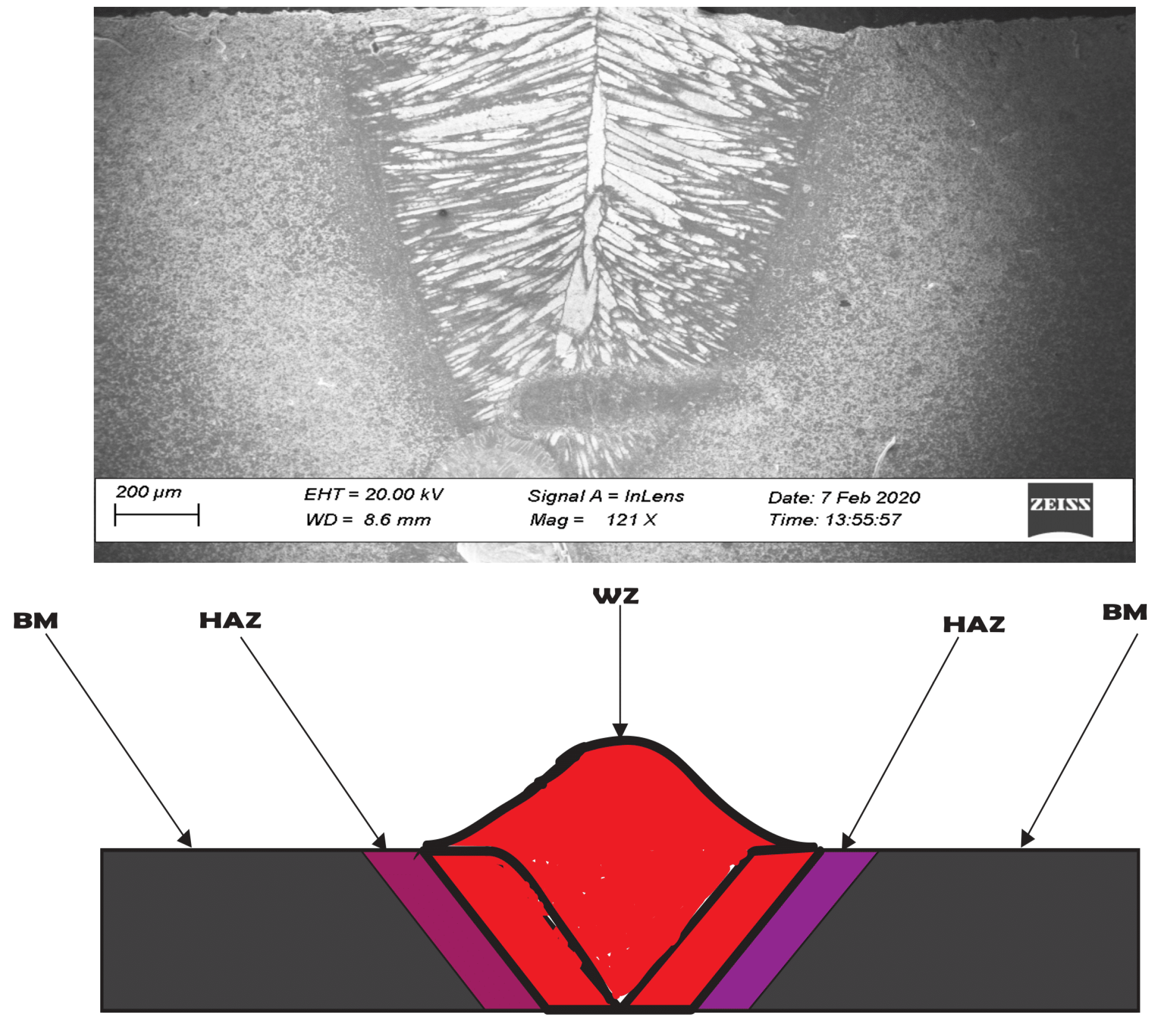
The importance of the WZ on the overall mechanical and chemical integrity of welded metallic alloy cannot be underestimated. Hu et al. [26] studied the mechanical and microstructure analysis of DSS welded using underwater hyperbaric FCA-welding process. From the study, it was noted that the WZ exhibited the highest microhardness with an estimated average value of 262 HV, compared to the other welded zones, such as the base metal (BM) and heat-affected zone (HAZ) [26]. Similar observations were seen in this research. Hence in the present study, the neural network algorithm was applied at the WZ for the microhardness prediction.

Therefore, the hardness at the WZ of a welded duplex stainless steel is a sophisticated task, necessitating an in-depth knowledge of all the processing parameters, including sintering and Nd: YAG welding parameters. Thus, the AI tool was used to estimate the hardness at the WZ. To this end, machine learning techniques, such as ANN and other algorithms, can be used to predict metallic alloy mechanical properties, such as Vickers hardness [22,27].

3. Experimental Process

3.1. Materials

Gas atomized and spherical (SAF2507) DSS powder of high purity of 91.5%, with an average particle size of 22 μm, was used as the starting material, obtained from Sandvik Osprey Ltd. (Neath, UK). The composition of the material is shown in

Table 1. Chemical composition of DSS powder.

Material	C	P	Si	Ni	N	Mn	S	Cr	Mo	Fe
2507	0.02	0.014	0.4	7.1	0.31	0.8	0.001	24.4	3.76	Balance

.

3.2. Spark Plasma Sintering Process

The SPS experiment was carried out with SPS equipment (model HHPD-25, FCT system GmbH, Frankenblick, Germany, situated at Tshwane University of Technology Pretoria, South Africa). However, before the sintering process, the gas atomized 2507 DSS powder was first pressed in 20 mm graphite die and punches, while a tungsten foil was used to separate the samples from the graphite tools. The samples were then sintered at the following temperatures 900 °C, 1000 °C, and 1100 °C at a pressure of 50 MPa under vacuum. A heating rate of 100 °C/m was considered for the sintering process, which lasted between 5–10 min. The SPS diagram is shown in Figure 1.

3.3. Laser Welding Process

Two specimens from the sintered 2507 DSS were sectioned using wire cutting (size: 12 mm × 12 mm × 3 mm), and later prepared in butt joint configuration. The laser welding equipment deployed was a JK 600 pulsed Nd:YAG laser welding machine at the Council for Scientific and Industrial Research (CSIR), South Africa. The laser process is shown in Figure 2. Welding parameters were selected based on the optimized parameters from the literature. The laser power and welding speed adopted in this study for samples A, B, and C were laser powers of 1500, 1700, and 2000 W, while the welding speed employed were 3, 3, and 2 m/min, respectively. Figure 3 shows the three distinct components of laser-welded metallic alloy, showing the base metal (BM), heat affected zone (HAZ), and weld zone (WZ). The processing parameters were fixed based on experimental trials and existing literature on Nd:YAG laser welding of duplex stainless steel.

3.4. Microhardness Test

Microhardness was carried out to measure the hardness of the welded samples. Vickers microhardness (HV) test was carried out using a Vickers microhardness (EM-700, Future Tech, Tokyo, Japan) tester, applying a load of 300 gf, with a dwell time of 10 s at room temperature. This research targeted the Vickers microhardness test at the welded zone (WZ). As the literature indicates, the chemical composition of the WZ is significant for the mechanical integrity of welded metallic alloy. The microstructure of the WZ differs from the base metal (BM) because of the variations in the chemical composition, as well as the thermal history of the WZ [28]. Therefore, the importance of the WZ to the welded joint overall mechanical integrity led to the consideration of using predictive tools to estimate the hardness of the WZ. An average of three spot hardness values were used and utilized in the neural network.

4. ANN Algorithm

In the material processing industry, it is pertinent for materials to undergo precise and consistent output, to meet the required quality standard set. The neural network has recently been used as a technique developed for processing elements, named neurons, that have connections with each other [9]. Given adequate data and algorithms, machine learning, with the help of a computer, can determine all known physical laws.

4.1. ANN Architecture

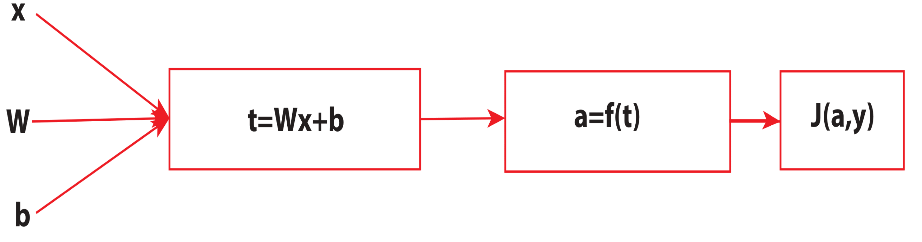
The last decade has witnessed a massive application of artificial neural networks (ANN) in many optimizations and prediction applications. ANN is classified as a highly nonlinear function and can capture very complicated patterns in data. Becoming the leading technique in machine learning and helped with complex engineering problems, including the prediction of the mechanical properties of materials. It can be represented by the following function, as indicated in Equation (1), where x is the input vector and $\widehat{y}$ is the prediction [29]. 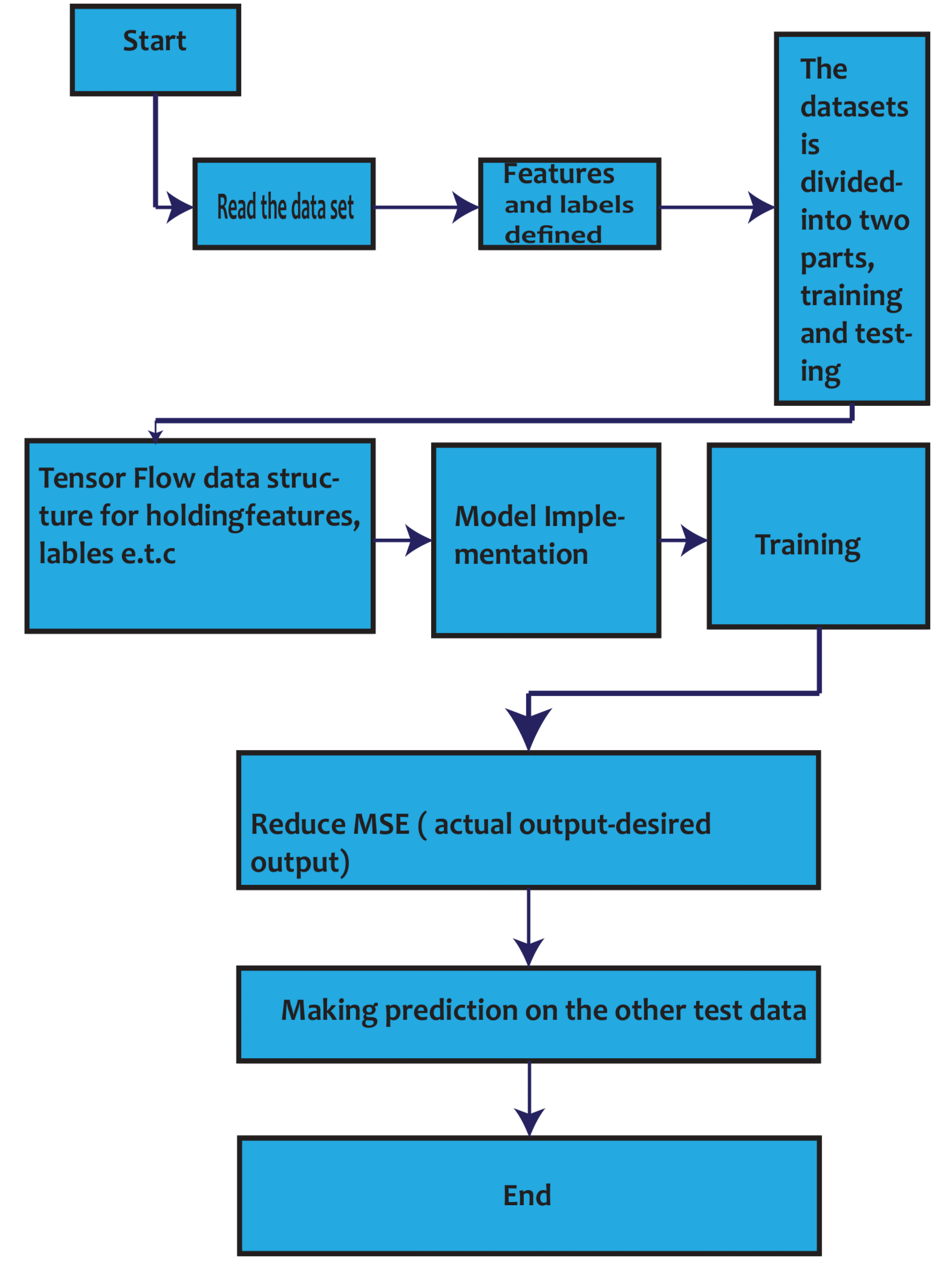Figure 4 shows the steps followed for the implementation of the use case.

$$\widehat{y}=f\left(x\right)=f^{\left(k\right)}(\dots .f^{\left(4\right)}\left(f^{\left(3\right)}\left(f^{\left(2\right)}\left(f^{\left(1\right)}\right))\right)\dots .\right)$$

(1)

The first layer is the input layer. It transfers information from the outside entity to the network, while the intermediate layers are the hidden layers. It also acts as the connecting link between the input and output layers by performing computation and transferring of information between the input and output layers. The last layer is the output layer, which is mainly responsible for the computations and relaying information outside the world. Therefore, these layers are made of neurons, which can be thought of as a simple computational unit that takes a weighted sum of input variables, sends the sum through an activation function, and finally, the output is the predictions. For the gradient descent equation, we have a linear transformation applied to an input $x$ by each neuron in the layers, as described by Equation (2), while Figure 5 presents the flow chart.

$$\mathit{t}\mathit{=}\mathit{W}\mathit{x}\mathit{+}\mathit{b}$$

(2)

where $\mathit{t}$ is a tensor, $\mathit{W}$ is called the weights, and the vector $\mathit{b}$ is the biases. The nonlinear transformation applied by each neuron is called the activation function.

4.2. Activation Function

The literature has many activation functions, such as the sigmoid, hyperbolic tangent, and rectified linear unit or ReLU. Meanwhile, the sigmoid and hyperbolic tangent is subjected to the so-called gradient vanishing.

ReLU activation has enjoyed wide application within neural networks, especially deep neural networks. At its inception, researchers were stimulated to use ReLU because of its biological resemblance. Meanwhile, the ReLU function later showed an improvement in the speed of neural network training, which eventually translated to good results. Its top-notch accurate predictive can be owed to its simplicity and function derivative. The derivative can be computed easily and does not have a vanishing gradient problem [25].

Here, we opted for the ReLU, mainly because it is piecewise and highly nonlinear. It provides better results than the sigmoid and hyperbolic tangents. Therefore, for this reason, it will be highly delightful to investigate how a ReLU function helps the networks to approximate functions.

The ReLU activation function is defined as:

$$f\left(t\right)=\max \left(0,t\right) and f^{∕}\left(t\right) \{\begin{array}{c} 1 if a>0\\ 0 otherwise \end{array}$$

(3)

$f\left(t\right)$ could be any activation function, depending on the problem at hand.

$$\widehat{y}=f^{\left(k\right)}\left(..f^{\left(4\right)}{b}^{\left(4\right)}+W^{\left(4\right)}{f}^{\left(3\right)}{b}^{\left(3\right)}+W^{\left(3\right)}{f}^{\left(2\right)}{b}^{\left(2\right)}+W^{\left(2\right)}{f}^{\left(1\right)}{b}^{\left(1\right)}+W^{\left(1\right)}x\right)$$

(4)

Figure 6 illustrates the ReLU activation function, while

Table 2. ANN parameters.

Model	Parameter	Value
ANN	Number of input layers	4
	Number of hidden Layers	2,3
	Number of output layer	1
	Maximum no. of epochs	750
	Activation function	RMSprop
	Learning rate	0.001

shows the parameters used in the ANN.

4.3. The Cost Function

Defining a loss or cost function is fundamental to any machine learning problem. During the training process, the interest is in the weight that minimizes the discrepancies between the estimated hardness values of the weld zone, in contrast to their actual training data values. This increases the accuracy of the network in predicting the new hardness value that is not from the training set. There are many cost functions, but the most widely used for regression problems is the mean square error. In introducing the mean square error cost function, a dataset was assumed:

$$\{\left(x_i,y_i\right){\}}_{i=1}^N$$

(5)

With the given pairs, i.e., features $x_i$ and corresponding target value $y_i \in ℝ$, the vector of the targets is denoted as $y_i \in {ℝ}^N$, such that $y_i$. is a target for object $x_i$. Similarly, $\widehat{y}$ $\in$ $ℝ$ denotes predictions for the objects: $\widehat{y}$ for objects $x_i$. The MSE loss function is as follows:

$$MSE\left(y,\widehat{y} \right)=\frac{1}{N}{\displaystyle \sum }_{I=1}^N{\left({\widehat{y}}_i-y_i\right)}^2$$

(6)

The goal of the learning algorithm would be to minimize the $MSE$ loss function. In the context of the deep neural network (DNN), this cost function will be written as follows:

$$J\left(\theta \right)=\frac{1}{N}{\displaystyle \sum }_{x\in X}(y-f(x;\theta )){ }^2$$

(7)

This is called the loss function of the DNN. The parameter theta ($\theta$) stands for the weights and biases that need to be optimized to minimize the loss function, and this is achieved through back-propagation.

4.4. Back-Propagation

Back-propagation can be described as a supervised learning algorithm for training multi-layer ANN. In this research work, back-propagation was used to compute the gradient of the loss function, as indicated by Equation (8).

$${\nabla }_{\theta }y={\nabla }_{\theta }J\left(x;\theta \right)$$

(8)

In addition, the choice of the network parameter does not affect the training data; back-propagation consists of finding the gradient of the network. Once the gradient is computed, gradient descent, or any related algorithm, could be used iteratively to minimize the loss function.

$${\theta }_k={\theta }_{k-1}+\in {\nabla }_{\theta }J\left(x;\theta \right)$$

(9)

where $\in$ is called the learning rate, and its value must be set meticulously for convergence reasons. Therefore, through the gradient, the errors are propagated in reverse in the network to adjust the parameter $\theta$ until the loss function reaches its minimum [30].

4.5. Optimizer

Recently, diverse methods have been initiated to effectively minimize the loss function by tracking the gradient and the second moment of the gradient. These methods include AdaGrad, AdaDelta, ADAM, and root mean square propagation (RMS prop). All these are available optimizers in Keras. In the RMS prop, to keep the running average of the first moment of the gradient, the second moment can be tracked or monitored through a moving average. Therefore, the update rule for the RMS prop is given by:

$$\begin{gathered} g_t={\nabla }_{\theta }J\left(\theta \right) \\ {s}_t=\beta s_{t-1}+\left(1-\beta \right)g_t^2 \\ {\theta }_{t+1}={\theta }_t+{\eta }_t \frac{g_t}{\sqrt{s_t+ϵ}} \end{gathered}$$

(10)

where β dictates the averaging time of the second moment and is usually taken to be about β = 0.9, ${\eta }_t$ is a learning rate typically chosen to be ${10}^{-3},$ and $ϵ~{10}^{-8}$ is a small regularization constant to prevent divergences. It can be inferred, from the Equation (10) above, that the learning rate is reduced in directions where the norm of the gradient is persistently large. The Convergence speeds up by enabling the use of a larger learning rate for flat directions [31].

4.6. Model Implementation and Learning

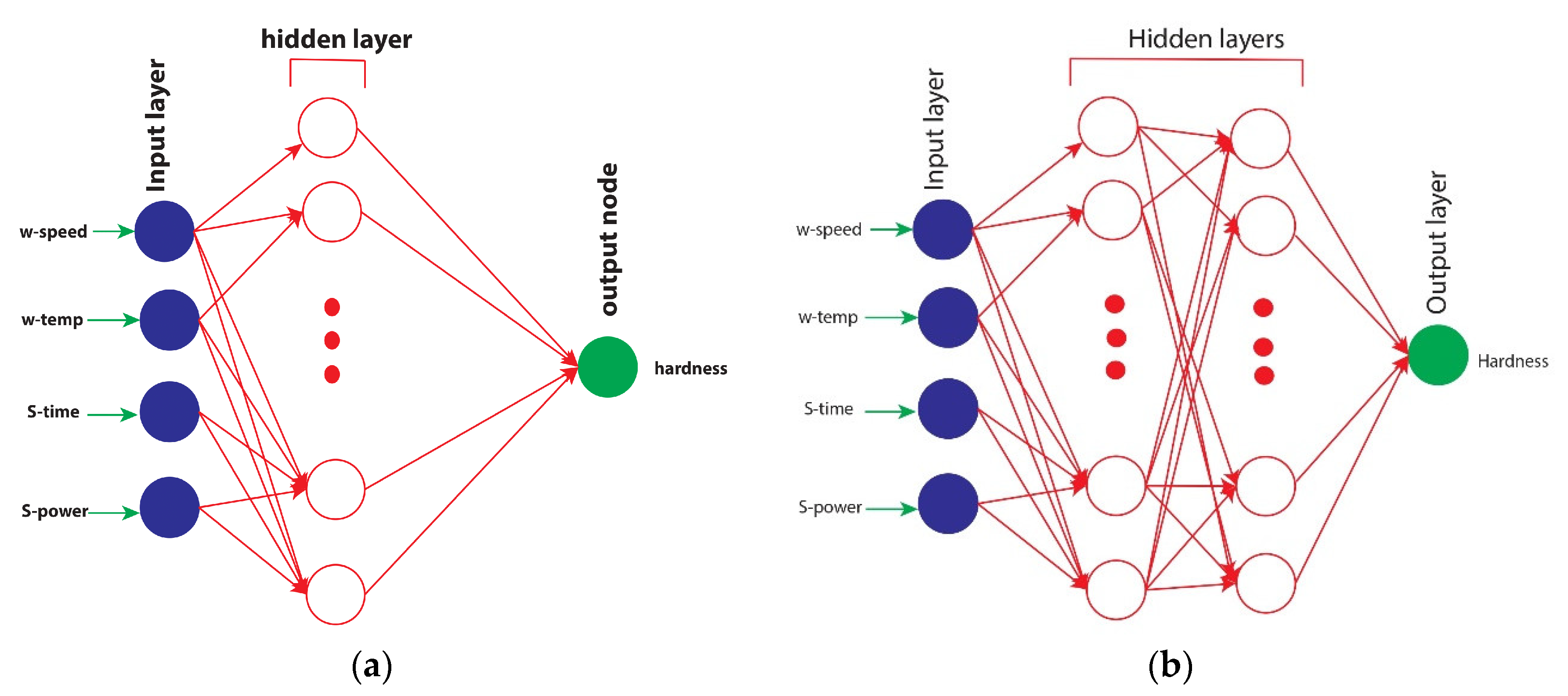
The ANN model was implemented in an open-source, Python-based, deep learning library called Keras with a google machine learning application. The TensorFlow framework was used as the back-end engine. ANN, with a back-propagation algorithm, was implemented with four input parameters, namely welding speed (w-speed), welding temperature (w-temp), sintering time (s-time), and sintering power (s-power). All these processing parameters influence the Vickers hardness of the welded sintered DSS alloy [32,33]. The authors have already published the data used for this analysis in Mendeley data [34]. These parameters, along with their ranges, are summarized in

Table 3. Parameters and their range used in the artificial neural network.

Parameter	Minimum	Maximum	Mean	Standard Deviation
S-temp	900	1100	1000	83.41
S-time	5.0	10	1733	2.41
Wel-power	1500	2000	1733	210
Wel-speed	2.0	3.0	2.67	0.48

.

The data obtained from the WZ of each sample was split into training and testing data, which was later used in the final evaluation of the model. The ANNS presented in this study utilizes one to two hidden layers, which are appropriate for the number of unique data, and has small data points; the ANN model was tweaked for different activation functions and training algorithms. Meanwhile, 80% of the data was selected as training data, while the rest was selected for testing. Before training and testing the network, the training datasets were normalized to avoid convergence of the model, thereby making the training more difficult, as well as, eventually, making the resultant model depend on the unit’s choice used in the input. ANN has no restriction on its training data, even with the fact that the magnitude of the measured data varies considerably. To achieve a more excellent training accuracy, it is better to put the training data source in the same order before proceeding with the analysis. Putting the training data in the same order before the training process is necessary. Therefore, the input and output variables were normalized to the range (0,1) by the following equation

$$X^{∕}=\frac{X-X_{min}}{X_{max}-X_{min}}$$

(11)

where $X$ is the original value, $X^{∕}$ is the normalized value, and $X_{max}$ and $X_{min}$ are the maximum and minimum of $X$, respectively.

Four neurons were fixed in the input layer corresponding to the input layer, with a hidden layer with variation between two and three layers. One neuron, corresponding to the one output, was fixed in the output layer, as shown in Figure 7a,b. An RMS prop optimizer was used to minimize loss.

The early stopping technique was used to improve the generalization property of the proposed neural network model. Additionally, early stopping was adopted to stop the training after a step of epochs elapses without showing improvement.

In this research, the number of hidden layers that perfectly provide us with the optimized neural network was obtained through trial and error by varying the training algorithm, activation function, and hidden layers.

The model was later compiled for the minimized MSE, RMSE, R², and MAE loss function, which was used as a metric to evaluate the prediction precision.

$$R^2=1-\left[\frac{{{\displaystyle \sum }}_i{\left(t_i-0_i\right)}^2}{{{\displaystyle \sum }}_i{\left(0_i\right)}^2}\right]$$

(12)

The model was later trained for 1000 epochs, and visualization of the training models was achieved using the statistics stored in the history.

5. Results and Discussion

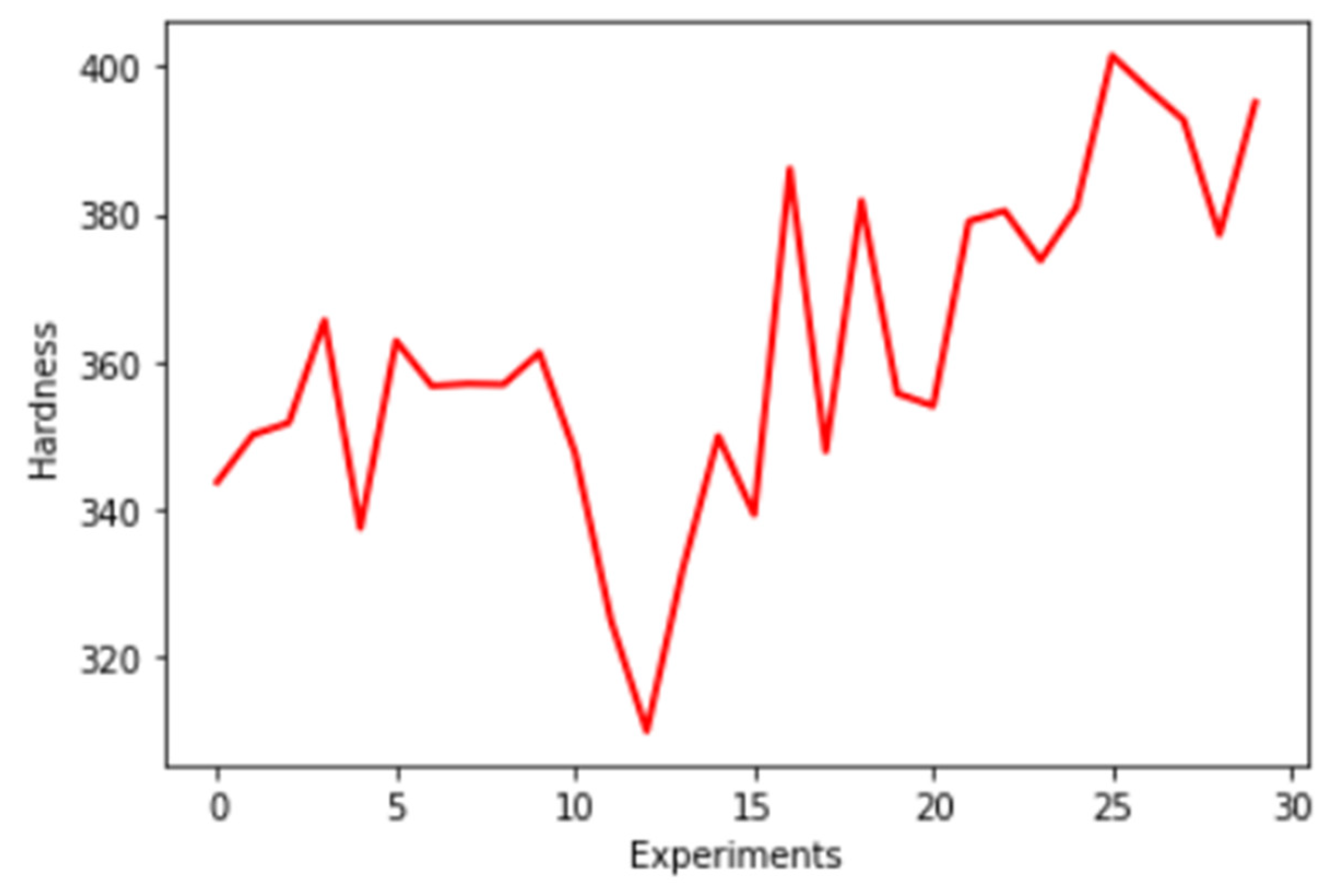
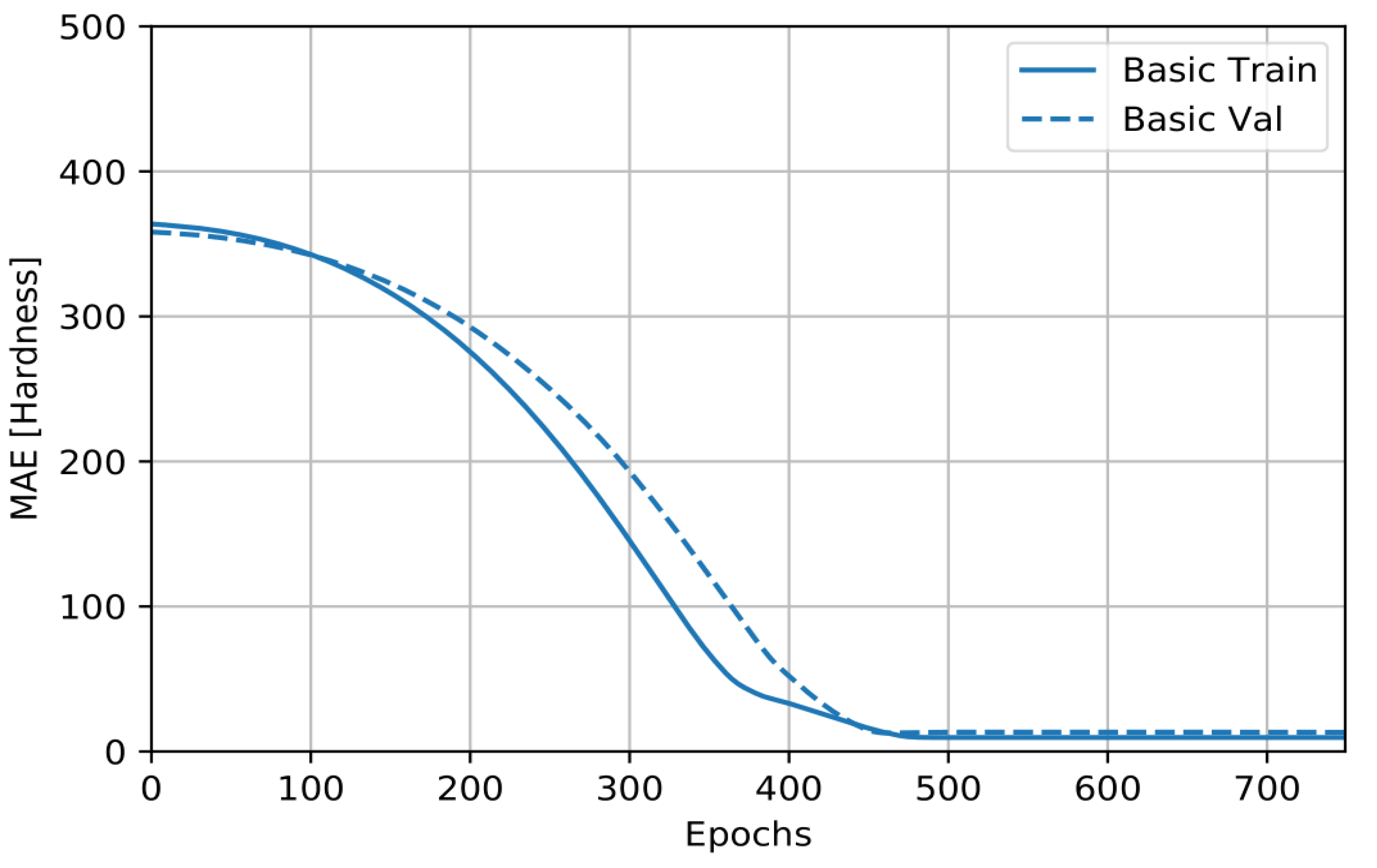
In the model proposed with four input layers, variations between two to three hidden layers with ReLU activation function were used. In the neural networks, the weights and biases were adjusted iteratively by using a training algorithm. Figure 8 shows the numbers of hardness values to be predicted varying from 312 HV to 400 HV. The most important performance metric used in this neural network was MSE [35].

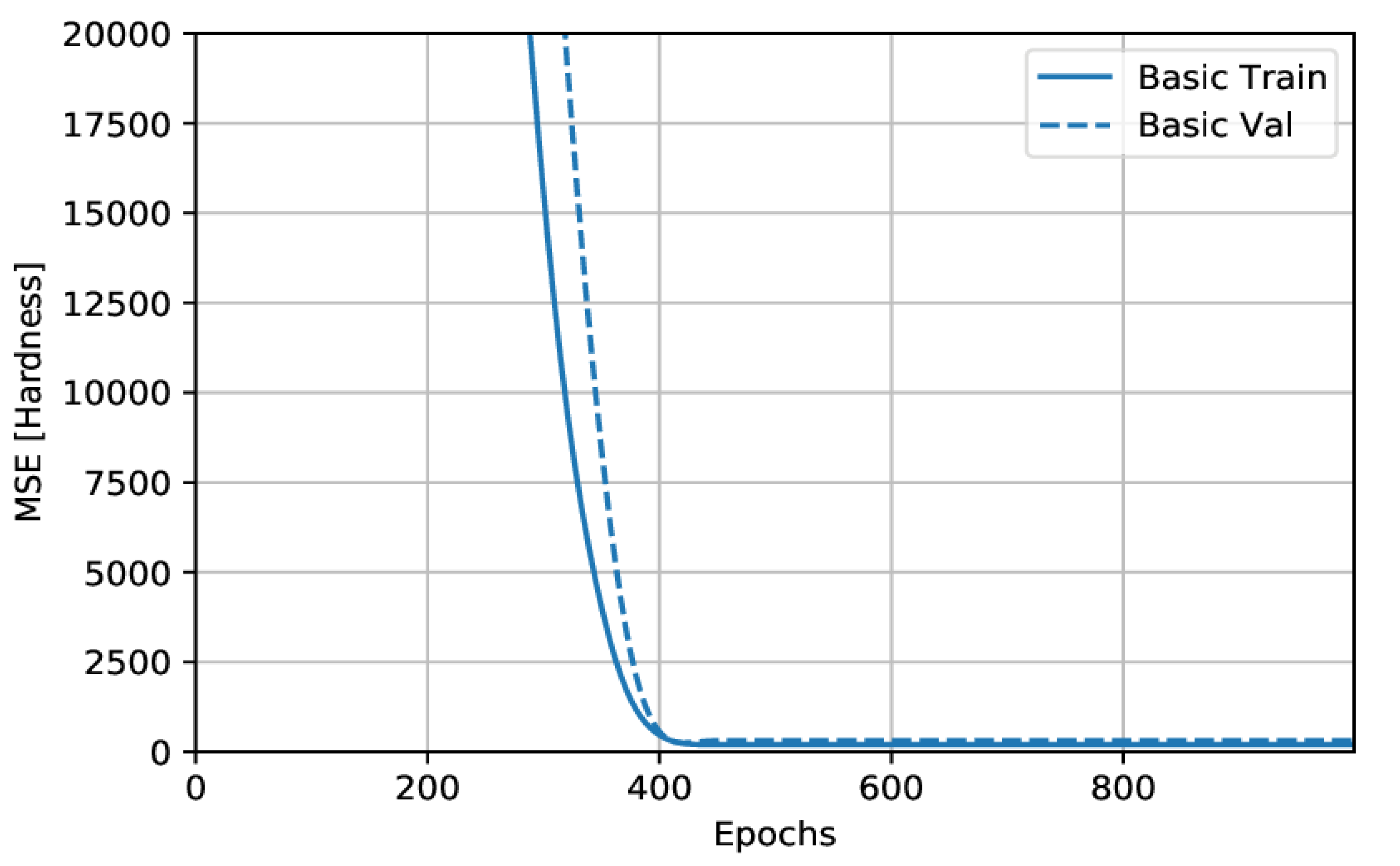
The MSE is a common loss function used for regression problems. Therefore, the basic training curve calculated from the training datasets provides an idea of how well the model is learning. The basic validation curve, calculated from a holdout validation dataset, provides an idea of how well the model is generalizing. Figure 9 and Figure 10 show little improvement, or even degradation, in the validation error after approximately 100 epochs.

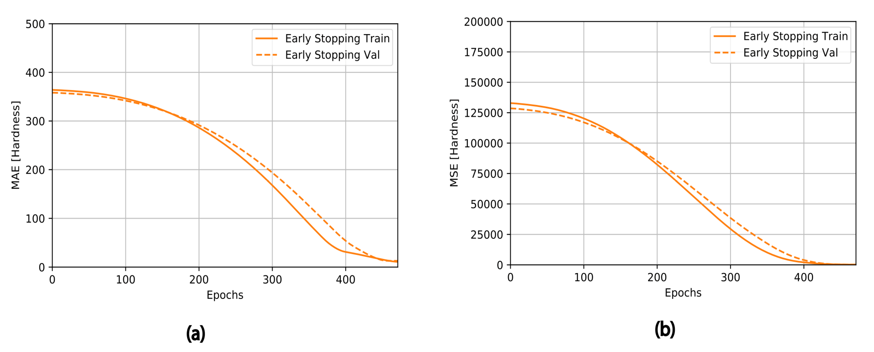
In other to improve the network generation, a combination of MSE and the mean square of the weights were minimized. Weights were also considered random variables, with Gaussian distribution. However, the early stopping callback was used to improve the generalization property of the different machine learning models proposed. If the set amount of epoch elapses without improvements, the early stopping callback automatically stops the training, as shown in Figure 11a,b. The plots show that the training process stopped as soon as the error validation set increased, showing the variation of MAE and MSE with varying epochs. In this research, R² and MAE were the metrics used to evaluate the predicting precision of the proposed models for both the test and training sets, as shown in

Table 4. Calculated values for R² and MAE for training and testing data.

Model	Training		Test
	R2	MAE	R2	MAE
Trial and error ANN
Hidden layers
2	0.43	9.6	0.54	15.42
3	0.41	10.50	0.57	15.42

[36].

Meanwhile, the different activation functions and optimizers available under the Keras API were tested, but the ones that could provide the best optimized predicted value were ReLU and RMSProp, respectively, with two and three hidden layers. As shown in Table 4, it is important to note that the model performed better when applied to the test set than when applied to the training set. The reason may be because training datasets have more data points than the test sets. Therefore, the probability of it containing a greater number of abnormal values is high, thereby significantly increasing the MSE that span from 2500 above. The best R² which is 0.54 and 0..43 respectively for both test and training with hidden layers 2 and R² values of 0.57 and 0.41 for the test, and training data with 3 hidden layers, explains the low ability of generalization. Meanwhile, The MAE values are lower in the training datasets with 0.43 and 0.41 for 2 hidden compared with 3 hidden layer architecture with MAE value of 15.42.

Table 5. Training predictions vs true values.

S.Number	True Values	Predictions	% Error
2	351.70	35.56	1.38
28	377.20	382.58	1.43
13	331.80	349.17	5.23
10	347.60	349.17	0.45
26	396.90	382.58	3.61
24	380.90	382.58	0.44
27	392.70	382.58	2.58
11	325.00	349.17	7.44
17	347.90	349.17	0.36
22	380.40	382.58	0.57
5	362.80	356.56	1.72
16	386.10	349.17	9.57
8	356.90	356.56	0.09
14	349.90	349.17	0.21
23	373.70	382.58	2.38
20	354.00	382.58	8.07
1	350.10	356.56	1.85
29	395.10	382.58	3.17
6	356.70	356.56	0.04
4	337.50	356.56	5.65
18	381.80	349.18	8.55
19	355.70	349.19	1.84
9	361.20	356.56	1.28
7	357.00	356.56	0.12

and

Table 6. Testing predictions vs true values.

S.Number	True Values	Prediction	% Error
0	343.70	356.56	3.74
3	365.70	365.56	2.47
12	310.00	349.17	12.64
15	339.00	349.17	2.91
21	379.00	382.58	0.95
25	401.0	382.58	4.69

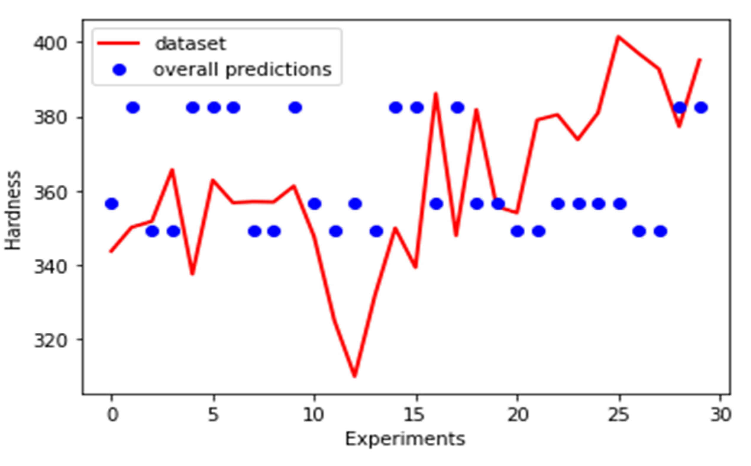
show the test and training predictions vs true values, respectively, showing their errors for the best predicted ANN architecture with two hidden layers. Figure 12 shows the plot of the actual and predicted values.

The minimum and maximum possible error values for the prediction of the hardness value were 0.09% and 9.57%, respectively. Clearly, with such a small dataset, a lack of generalization is expected, which warranted the use of another metric to appreciate how well the model is at prediction. The percentage error was computed on each prediction, according to the Equation (10). $TV$ is the target value, and $PV$ is the predicted value.

$$PE=100\times \frac{\left|TV-PV\right|}{TV}$$

(13)

Figure 12 shows how the variations of actual hardness value versus ANN predicted results for hardness. This shows the disparity between the actual datasets points to the predicted values graphically.

6. Conclusions

This research developed a predictive model, to predict the hardness value. Meanwhile, the predictive model was developed using a neural network with an RMS prop optimizer and ReLU activation, which seems to be the best parameter selected. This is also justified in the cited research [24]. The hidden layers were varied from two to three layers to predict the hardness value. Through the linear regression analysis, it can be inferred that the predicted and real values did not deviate too much. Empirical examinations of the predicted hardness value (by comparisons of predicting measures, such as MSE and MAE) show that the proposed neural network improves the precision of predicting the hardness of the welded metallic alloy.

It can be noticed that the evolution of MSE with the training and test data of the ANN suggested no overfitting of the ANN. However, the study cannot guarantee the top-notch performance of the ANN model, as the R² achieved in the test data was greater than that of the training data. This may be because there is not much numerical diversity in the input data used. Hence, the anomalous values might be more noticeable in the training sets than the test sets, given their larger dimension, compared to the test sets, which increases the R² value of the test sets.

Forecasts of the hardness value were acceptable from the technological viewpoint. To enhance the reliability of the model and improve the predictive performance of the ANN model, it is important to use an increased number of data points for the training, testing, and validation process.

Lastly, this research work proposes that the full integration of the analysis and prediction into one framework is possible.