Article

Towards the Determination of Machining Allowances and Surface Roughness of 3D-Printed Parts Subjected to Abrasive Flow Machining

by
Mykhailo Samoilenko
1,
Greg Lanik
2 and
Vladimir Brailovski
1,*
1
Department of Mechanical Engineering, École de Technologie Supérieure, 1100 Notre-Dame Street West, Montreal, QC H3C 1K3, Canada
2
Extrude Hone LLC, 235 Industry Blvd., Irwin, PA 15642, USA
*
Author to whom correspondence should be addressed.
J. Manuf. Mater. Process. 2021, 5(4), 111; https://doi.org/10.3390/jmmp5040111
Submission received: 27 September 2021 / Revised: 8 October 2021 / Accepted: 14 October 2021 / Published: 17 October 2021
(This article belongs to the Special Issue Advanced Surface Finishing Processes)

Abstract

:
Abrasive flow machining (AFM) is considered as one of the best-suited techniques for surface finishing of laser powder bed fused (LPBF) parts. In order to determine the AFM-related allowances to be applied during the design of LPBF parts, a numerical tool allowing to predict the material removal and the surface roughness of these parts as a function of the AFM conditions is developed. This numerical tool is based on the use of a simplified viscoelastic non-Newtonian medium flow model and calibrated using specially designed artifacts containing four planar surfaces with different surface roughnesses to account for the build orientation dependence of the surface finish of LPBF parts. The model calibration allows the determination of the abrasive medium-polished part slip coefficient, the fluid relaxation time and the abrading (Preston) coefficient, as well as of the surface roughness evolution as a function of the material removal. For model validation, LPBF parts printed from the same material as the calibration artifacts, but having a relatively complex tubular geometry, were polished using the same abrasive medium. The average discrepancy between the calculated and experimental material removal and surface roughness values did not exceed 25%, which is deemed acceptable for real-case applications. A practical application of the numerical tool developed was demonstrated using the predicted AFM allowances for the generation of a compensated computer-aided design (CAD) model of the part to be printed.

Graphical Abstract

1. Introduction

In recent years, additive manufacturing (AM), or 3D printing, became a widely used and rapidly developing technology that simplifies the production of complex parts with reduced weight and improved functionality. At the same time, laser powder bed fusion (LPBF) became one of the most mature technologies for the 3D printing of metal parts. Despite the advantages presented by LPBF, an excessive as-built surface roughness inherent in the process impacts the fluid flow and the heat transfer characteristics of LPBF parts, and alters their mechanical properties. Strano et al. [1] studied the impact of the LPBF build orientation on the surface topography, while Kruth et al. [2] provided a detailed explanation of mechanical limitations associated with the surface finish of LPBF parts. They determined that the bigger the angle between the surface of a printed part and the building platform, the higher the surface roughness. For example, as reported by Urlea and Brailovski [3], if the build angle of a Ti-6Al-4V component increases from 0 to 135°, the as-printed surface roughness R a increases from 4 to 23 μm.
Different approaches and techniques were developed to improve the surface roughness of LPBF parts. For example, Yadroitsev and Smurov [4] improved the surface finish by optimizing the laser scanning strategy. From their side, Cherry et al. [5] considered the improvement of the as-built surface roughness by varying the scanning speed. However, for most applications, the as-built surface roughness still requires additional surface finishing. In this context, Alrbaey et al. [6] proposed the use of the surface laser melting-remelting strategy, but this approach is limited to upper surfaces of printed parts. Urlea and Brailovski [7] worked on electrochemical polishing of LPBF parts, but pointed out the difficulty of electropolishing parts with intricate internal geometries, such as internal cavities and channels. To overcome the latter difficulty, chemical polishing appears to be a promising alternative, since it facilitates access to difficult-to-reach surfaces. However, as shown by Pyka et al. [8], chemical polishing alone cannot entirely eliminate the LPBF surface imperfections. To improve the preceding technique, Mohammadian et al. [9] combined the chemical and the abrasive flow polishing techniques to polish 3D printed parts but pointed out the risks of surface contamination, as well as the health and environmental hazards related to the use of chemicals.
Considering the above, forced flow of a chemically passive abrasive medium across the surface of a part to be polished can be considered as an effective and safe surface finishing technology for LPBF parts and particularly those with complex internal channels. As discussed by Rhoades [10], this process called abrasive flow machining (AFM) has been used for decades to deburr, polish or radius surfaces and edges of parts with complex outer and internal shapes. For example, Cheng, et al. [11] studied AFM of gas turbine engine blades, while Ferchow et al. [12] used this technology to polish curved channels of 3D-printed nozzles.
It should be noted that abrasive media used in AFM mainly consist of a liquid polymer carrier and dispersed abrasive particles. Kumar and Hiremath [13] reviewed the AFM media applications and found that the mostly used polymer carriers are polyborosyloxane and silicone rubber, while for abrasives, they are silicon and boron carbides, aluminum oxide, and polycrystalline diamond particles. A typical abrasive particle size lies in the range of 32–1035 μm, as mentioned by Trengove [14], while concentration of the abrasive may approach 80%, after which the medium begins to act inefficiently, as demonstrated by Kar et al. [15]. An interesting method to assess the cutting forces of abrasive flow machining using a two-phase viscoelastic flow approach was proposed by Dong et al. [16] This method combines an analytical model for calculating the cutting factors and an experimental technique to calibrate this model. While this approach provides an interesting insight into the abrading behavior of AFM media and offers a new perspective for the optimization of the media composition, it cannot directly be applied to predict the material removal (MR) during the AFM process and, therefore, to determine the machining allowances of the parts to be polished.
As indicated by Bouland et al. [17], this last endeavor represents the main challenge in the use of AFM for the finishing of 3D-printed parts. Thus, a numerical tool allowing the MR and the surface roughness prediction, depending on the AFM process parameters and the geometric and material attributes of the part to be polished, is required. Different computer fluid dynamic-based AFM MR models were reviewed when preparing this paper. Jain et al. [18] proposed to calculate MR using an analytical model that considers the material hardness, the abrasive grain size and concentration, the normal stresses and the velocity of a Newtonian (linear viscosity) fluid. Wan et al. [19] extended this formulation by adopting a non-Newtonian fluid (power law) model and introducing the MR dependence on the initial and limiting surface roughnesses. Cheng, Shao, Bodenhorst and Jadva [11] also used the non-Newtonian fluid model, but in this case, they reduced the MR model formulation by using experimentally found constants dependent on the media type and the workpiece material and a variable flow shear rate.
Upon close examination, all these models represent the application of a classical theory of metal-cutting processes, with the main challenge consisting in an adequate computational fluid dynamics (CFD) simulation of the AFM media flow across the surface of a part to be polished, and allowing the calculations of the velocity and force fields acting on this surface. However, in all these models, the AFM medium is simulated as a purely viscous fluid, thus neglecting the fact that it should rather be considered as a viscoelastic fluid, as indicated by Uhlmann et al. [20]. However, no publications that account for the viscoelastic behavior of AFM media were found at the time of writing. Moreover, as can be found in Dash and Maity [21], no-slip boundary conditions are generally applied on walls during the CFD analysis of the AFM process, which contradicts the assessment of Uhlmann et al. [22] that slip cannot be neglected while simulating flow of viscoelastic fluids.
Based on the above considerations, the ultimate goal of this study is to develop a numerical model allowing the prediction of AFM allowances and the generation of compensated 3D CAD models of LPBF parts as a function of the selected AFM media, process parameters and required surface finish.

2. Methodology

2.1. AFM Process Numerical Modeling

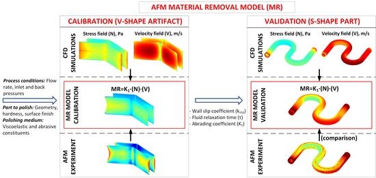
2.1.1. Material Removal Model: General Formulation

From the theory of metal-cutting processes described in [23], the volume of the material removed M R v (m3) may be calculated as:
M R v = 1 E 1 P c · l = K 1 · P c · v · t
where   P c is the cutting force, N; E 1 is the specific energy required for cutting, J/m3 ; K 1 is the material removal factor (as shown by Brinksmeier et al. [24], K 1   corresponds to the Preston coefficient from the theory of abrasive polishing), m3/J; l is the distance over which the cutting force acts, m; v is the cutting velocity, m/s; and t is the time, s.
By analogy with Equation (1), the thickness of the material removed during AFM, M R t (m), could be expressed as a function of the cutting stress N (Pa) and the abrasive medium velocity v   ( m / s ) at each segment of the polished body, and the time of polishing, t   ( s ):
M R t = M R v A c = K 1 · P c A c · v · t = K 1 · N · v · t
where A c is the surface of the cutting segment, m2.
The abrading (cutting) coefficient K 1 , as well as the cutting stress N and velocity v fields, depend on the following characteristics:
  • Polished part hardness and geometric attributes (shape and surface roughness);
  • Rheological properties of the abrasive medium that depend on its composition (type of the viscous carrier + type and concentration of abrasive particles) and the temperature of use;
  • AFM operation conditions: inlet and back pressures.

2.1.2. CFD Simulations: Simplified Viscoelastic Model

For a given “abrasive medium/polished part” combination, the M R t prediction requires the knowledge of the abrading coefficient K 1 and the v and N fields generated by a flow of the abrasive medium across the surface of the part to be polished. To calculate the unknown v and N fields, ANSYS Polyflow software was selected. Three CFD models proposed by ANSYS Polyflow were evaluated: the generalized Newtonian model, the differential viscoelastic model and the simplified viscoelastic model. The first two models were excluded from consideration because the generalized Newtonian model could not predict normal stresses and the differential viscoelastic model was too computationally expensive. Moreover, as described by Walters and Webster [25] and Niethammer et al. [26], the latter presents numerical difficulties for CFD modeling with high Weisenberg numbers ( W e > 1 ), and under some flow conditions of this study, W e   can indeed reach a value of 140.
Based on the above considerations, the simplified viscoelastic ANSYS Polyflow model was ultimately selected to solve the momentum (3) and the incompressibility (4) equations:
p + · T + f = ρ a
· v = 0
where   p is the pressure, Pa; T is the total extra-stress tensor, Pa; f is the volume force, N; ρ is the density, kg/m3; a is the acceleration, m/s2; and v is the velocity, m/s. The shear and normal stresses acting on the viscoelastic element are shown in Figure 1:
Macosko [28] describes that the first normal stress difference ( N 1 ) is necessary to keep the block at a constant thickness x 2 , at this T 11 T 22 0 :
N 1 = T 11 T 22
As shown in Figure 1, three normal stresses act on the element ( T 11 , T 22 , T 33 ) and, therefore, the second normal stress difference N 2 is:
N 2 = T 22 T 33
For an ideal rubber N 2 = 0 , whereas for real polymers, N 2 is typically much smaller as compared to N 1 . As a result, for a simple shear flow, the simplified viscoelastic model incorporates N 1 into the force balance and takes T 22 = T 33 = 0 , such that the total extra-stress tensor T is given by:
T = T 11 T 12 T 13 T 21 T 22 T 23 T 31 T 32 T 33 = ψ · μ χ ˙ · χ ˙ η γ ˙ · γ ˙ 0 η γ ˙ · γ ˙ 0 0 0 0 0
where η γ ˙ · γ ˙ is the shear stress component, Pa; ψ · μ χ ˙ · χ ˙ is the first normal stress, Pa; η γ ˙ is the shear-rate dependent viscosity, Pa∙s; μ χ ˙ is the normal viscosity, Pa∙s; γ ˙ is the shear rate, 1/s; χ ˙ is the viscoelastic variable, 1/s; and ψ is the weighing factor.
To express both the shear rate-dependent η γ ˙ and normal μ χ ˙ viscosities of an AFM medium, the Carreau–Yasuda model of a non-Newtonian fluid was adopted:
η γ ˙ = η + η 0 η 1 + λ γ ˙ a n a a
μ χ ˙ = η + η 0 η 1 + λ χ ˙ a n a a
where η 0 is the fluid viscosity at zero shear rate, Pa∙s; η is the fluid viscosity at infinite shear rate, Pa∙s; λ is natural time, s; and n and a are the power-law indexes. As a result, the first normal stress difference ( N 1 ) becomes:
N 1 = T 11 = ψ · μ χ ˙ · χ ˙
where the viscoelastic variable χ ˙ obeys the transport equation involving the characteristic (relaxation) time τ γ ˙ , which is given by:
τ γ ˙ D χ ˙ D t + χ ˙ = γ ˙
The Equation (11) is such that the solution χ ˙ = γ ˙ is recovered in simple shear flow.

2.2. AFM Process Experimentations

2.2.1. Materials and Parts

For this project, an LV-60B medium (Extrude Hone LLC, Irwin, PA, USA) composed of a viscous carrier (PBS, polyborosiloxane) and an abrasive charge (B4C, boron carbide with d g = 360   μ m ) in 37.15:57.85 (wt.%) proportions, was selected as recommended by Extrude Hone experts based on the polished geometry analysis. Rheological measurements of the complex viscosity η * γ ˙ , storage modulus G γ ˙ and loss modulus   G γ ˙ of the medium were carried out using a HR-2 discovery hybrid rheometer (TA Instruments, New Castle, DE, USA), with a parallel plate–plate setup ( d = 25   mm ; t = 1   mm ). To control the slip conditions, a sandpaper (grit 120) was attached to the plates, as recommended by the rheometer manufacturer in the training manual [29]. The following protocol was used: (a) Conditioning: 25 °C soak time for 10 s followed by pre-shear performed at a shear stress of 100 Pa for 60 s, followed by final equilibration for 300 s; (b) Frequency oscillation: 25 °C soak time for 60 s followed by testing under a standard controlled stress of 800 Pa with a logarithmic sweep (angular frequency: 628.3–1 rad/s; 10 points per decade); (c) Data acquisition: conditioning and sampling times 3 s; 64 points in waveform; 0.0 µN∙m controlled flow torque, and (d) Conditioning at end of test: 25 °C temperature re-set.
Two types of 3D-printed parts were designed to support the model development: (a) V-shape artifact for model calibration (Figure 2a); S-shape specimen for model validation (Figure 2b). The calibration artifact was designed to reflect the dependence of the surface roughness of LPBF parts on their build orientation. To this end, the V-shape artifact contains four distinct zones, A, B, C and D, which correspond to the build orientation angles of 90°, 45°, 90° and 135°, respectively. At the same time, the V-shape artifact possesses a simple flat-plane geometry facilitating measurements of its surface roughness and dimensions. The S-shape specimen was designed to represent one of the most typical 3D parts, namely, tubular channel components for conformal cooling applications. To facilitate inspection, the S-shape specimen (Figure 2b) is divided into two halves (top and bottom) to be assembled before polishing. To obtain identical initial surface roughness distributions ( R a 0 ) in the top and bottom halves of the specimen before polishing, their semi-channels were oriented upward during printing, thus providing a symmetrical build angle variation of 0° to 90° in both of them.
All parts in this study were manufactured using an EOSINT M280 400W Ytterbium fiber laser powder bed fusion system (EOS GmbH, Munich, Germany), an EOS StainlessSteelCX powder, and a “Customized CX” parameter set with a 30 μm layer thickness. After printing, based on the EOS [30] recommendations, the parts were annealed at 850 °C for 30 min under argon atmosphere to relieve residual stresses caused by the process, and cut from the building plate. The V-shape artifacts were divided into two groups: the first group was kept in the as-built state and all A, B, C and D surfaces of the second group were mechanically pre-polished down to R a = 1.0   μ m before AFM. The reason for creating the two groups of V-shape artifacts was the need to separate the influence of the overall part geometry on the material removal during the AFM process from that of its surface roughness. As it will be demonstrated herein, the pre-polished artifacts were used for the calibration of the material removal ( M R t ) model, whereas the as-built artifacts were used for the extraction of the R a M R t evolution function.

2.2.2. AFM Setups

Two AFM setups were used in this study, one dedicated to the AFM processing of V-Shape artifacts (calibration setup, Figure 3a), and the second, to the AFM processing of S-shape specimens (validation setup, Figure 3b). Note that the first setup was built as a laboratory testing rig, while the second setup represents a commercially available industrial-size piece of equipment.
The AFM calibration setup (Figure 2a) is shown in Figure 3a and described in details in [17]. Briefly, under the action of the two moving pistons (1), an AFM medium flows reciprocally from the two feeding chambers (2) into the fixture (3) holding the V-shape artifact (4). The V-Shape pre-polished and as-built artifacts were polished under the same AFM conditions (flow rate 31.18 × 10 5   m 3 / s ; duration up to 300 cycles). The polishing process was discretized as follows: 302, 454, 756, 1512, 3024, 6047, 7559 and 9071 s (10, 15, 25, 50, 100, 200, 250 and 300 sequential passes). After each polishing sequence, the V-shape artifact was removed and evaluated (weighing, M R t profile and R a measurements). During the V-shape calibration trials, RAW data ( p inlet ) were captured with 1 s intervals using a custom LabView-based system. Note that since the pistons (1) (Figure 3a) move back and forth under the action of a single actuator (moving assembly), this setup does not allow for the controlled application of back pressure during polishing.
The AFM validation setup (Figure 2b) is shown in Figure 3b and reproduces an industrial piece of AFM equipment, Vector 150 (Extrude Hone LLC, Irwin, PA, USA). In this case, the force was applied only by one piston at a time ( p inlet = 1200   psi ), such that the second piston moved under the pressure exerted by the polishing medium. Although no specific back pressure was applied to the second piston, an effective positive p back existed due to an unspecified AFM system resistance. The polishing process was discretized as follows: 2966, 2211, 1787, 5272, 6398, 11,287, and 10,760 s (1, 1, 1, 4, 5, 7 and 7 sequential passes). After each polishing sequence, the S-shape validation specimen was removed and evaluated (weighing and R a measurements). During the S-shape trials, RAW data ( p inlet , p back , flow rate Q ) were captured with 0.5s intervals using pressure sensors (3100 30CPS (Gems, Plainville, CT, USA), 0–3000 psi) and linear encoders (flow rate measurements) connected to a dedicated data acquisition system.

2.2.3. Measuring Equipment and Protocols

Before and after polishing, the V- and S-shape parts were weighed using electronic scales SECURA324-1S (Sartorius, Goettingen, Germany) and AP-210 Analytical Plus (Ohaus, Parsippany, NJ, USA), both 0.1 mg. Next, the R a and M R measurements on the V-shape artifacts were carried out after each polishing series using a VR-5200 3D optical microscope (Keyence, Osaka, Japan) (12× magnification, high resolution, fine mode, ±2.5 μm) and Keyence VR-5000 series software. On the other hand, the R a measurements on the S-shape specimens after each polishing series were carried out using a Surfcom 1500SD3 surface roughness tester (Accretech, Tokyo, Japan) with an DM43825 stylus (Accretech, Tokyo, Japan) (tip radius 2 μm), while the 3D optical microscope M R and R a measurements on these specimens were carried out for their initial and final states only.
MR measurements, V-shape: As an example, Figure 4 illustrates the M R measurements realized on a 90°-oriented surface A of the V-shape artifact (Figure 4a). The same routine was repeated for the resting 45°-, 90°- and 135°-oriented surfaces. For these measurements, the initial and polished (final in this case) states were first compared using a reference plane passing by two zones located at the left and right edges of the artifact, which were not subjected to polishing (Figure 4a). A “volume and area” module of the 3D microscope software was then used (see Figure 4b) to determine the void ( V void , mm3) and solid ( V s , mm3) volumes, the first corresponding to the void located below the reference plane, while the second corresponded to the material located above the reference plane. For a given number of passes ( n ), the corresponding material removed volume M R v , n was determined according to Equation (12):
M R v , n = V void , n V void , 0 + V s , 0 V s , n
To determine the M R t value at each point of the surface, the corresponding initial and final AFM point clouds were exported from the 3D microscope into the CATIA software environment and aligned together using a 3D CAD model of the part. The M R t calculations were performed in the MATLAB environment using a customized point-by-point calculation routine based on the “findNearestNeighbors” function.
MR measurements, S-shape: For the M R t measurements on the S-shape specimens, the corresponding initial and final (AFM) point clouds were divided on the “base”/“channel” regions (Figure 5a) and exported from the 3D microscope software. Because of the complexity of the profile measured, the alignment routine was realized using the “Align” module in the MeshLab software environment. The initial state was selected as the reference and the base regions were used for alignment. Then, the matched channel STL point clouds (Figure 5b) were exported for point-by-point M R t calculations in the MATLAB environment. For the model validation, the experimentally found V- and S-shape M R t fields were assigned to the corresponding CFD mesh vertices.
Ra measurements, V-shape: To establish the R a M R t function, the same reference planes as for the M R v measurement were used (Figure 4a). However, for this study, 8 × 8 mm segments with a relatively uniform M R t evolution on each of the surfaces ( M R t , n ) were selected, as shown in Figure 6a. Next, the “Multiline roughness” module of the 3D microscope with 30 equally spaced (~250 µm) lines was used to calculate the average R a (Figure 6b). The   M R t , n was found as defined by Equation (13):
M R t , n = M R v , n / A segm
where A segm = 64   mm 2 : area of the segment studied.
Ra measurements, S-shape: In addition to the R a measurements for building angles 0° and 40° realized after each polishing series using a surface roughness tester (see Figure 7, region of interest ROI), these measurements were repeated using a 3D microscope as shown in Figure 8a (straight channel ROI), by positioning the specimens at an angle of 45°. The “Cylinder” surface shape correction was then applied in the 3D microscope software to determine the R a corresponding to a build angle ( α ) varying from 0 to 90° (Figure 8b).

2.3. CFD Simulation, Model Calibration and Validation

2.3.1. CFD Simulation Setups

The V- and S-shape CFD simulation setups are presented in Figure 9a,b and the corresponding CFD parameters are presented in Table 1. Each CFD setup represents a symmetrical system divided into two volumes: polishing volume and global volume, with the former corresponding to the zone containing a part subjected to polishing, either V- or S-shape, and the latter corresponding to the remaining zone of an entire AFM setup. For each system, the boundary conditions (BC) on walls were also divided into two corresponding BC setup conditions, with and without a part to be polished. For the CFD analysis, the media rheology [ η γ ˙ , τ ], the inlet flow rate ( Q ), the back pressure ( p back ) and the wall slip coefficient ( k slip ), characterizing friction between the abrasive medium and the polished part, were used as input parameters, whereas the simulated inlet pressure ( p inlet ) was used as a control parameter.
During the CFD analysis, simulations were performed by swapping the inlet/outlet boundary conditions (BC). The justification for this swapping was two-fold: (a) each of the modeling cases represents the actual back and forth movements during the AFM process and (b) the simulated normal stress fields ( N 1 ) of the simplified viscoelastic model are sensitive to the surfaces, either inlet or outlet, to which the BC are applied. Next, the average (back + forth)/2 solutions were obtained. To reduce the computational cost, “symmetry” BCs (boundary conditions) were applied during the simulations of 3D volumes, which resulted in a 50% reduction in the actual ( Q real ) inlet flow rate ( Q CFD = Q real / 2 ). The following assumptions were made to facilitate the simulations:
  • Identical time rate dependences for the first normal μ χ ˙ and shear-rate η γ ˙ viscosities;
  • Constant values for the relaxation time, τ γ ˙ = c o n s t . As a first approximation, τ γ ˙ was taken at the cross-over of the G and G graphs and then calibrated using the M R results obtained with the pre-polished V-shape artifacts.

2.3.2. Model Calibration and Validation

Following the CFD sensitivity study on V-shape artifacts, the wall slip coefficient ( k slip ) and the material relaxation time ( τ ) were found to have the most impact on the CFD simulation results ( v , N 1 ) with k slip influencing primarily the p inlet and the v and N 1 fields and τ influencing primarily the N 1 field. Therefore, for the MR model calibration, k slip and τ were chosen as independent variables, and the M R t solution was established in the form:
M R t = K 1 · N 1 k slip , τ · v k slip · t
The removed material thickness ( M R t ) and time ( t ) of the AFM process are considered as control parameters, since they could be determined directly from experiments. In contrast, K 1 as well as k slip and τ are unknown parameters requiring calibration. Thus, the MR model development is divided into two phases (see Figure 10):
  • The model calibration phase using two types of V-shape artifacts:
    (a)
    The pre-polished V-shape artifact serves for the calculations of the stress and velocity fields of the polishing medium, and it is realized in two steps:
    -
    First step: k slip calibration. The entire AFM setup containing the V-shape artifact (Figure 9) is considered to be fully polished and having an identical and constant k slip = k pol coefficient, irrespective of the polishing stage. The k slip value is adjusted to equalize the simulated and the experimentally-measured inlet pressures: p inlet , CFD = p inlet , exp , and then applied as the BC on walls.
    -
    Second step: τ and K 1 calibration. The relaxation time ( τ ) and the material abrading coefficient ( K 1 ) are adjusted to reach the best fit between the numerically predicted ( M R t , mod ) and the experimentally measured ( M R t , exp ) material removal values. To assess the degree of fitness, the maximum coefficient of determination ( R 2 ) corresponding to the proportion of variance between the dependent and independent variables is found according to Chicco et al. [31] as:
    R 2 = 1 i = 1 n M R t , mod M R t , exp 2 i = 1 n M R ¯ t , exp M R t , exp 2
    (b)
    The as-built V-shape artifact is used to establish the dependence of the experimentally measured surface roughness on the numerically calculated material removal, R a M R t , R a 0 , where R a 0 is the initial (as-built) wall roughness.
  • The model validation phase using S-shape specimens: At this stage, the k slip and τ values and the calibrated M R rate N 1 , v and R a M R t ,   R a 0 models are used to calculate the material removal and the surface roughness at each point of the S-shape specimens during their polishing, and the results obtained are compared with their experimentally obtained equivalents to conclude on the validity of the proposed modeling approach.

3. Results

3.1. Rheology of the LV-60B Abrasive Medium

The results of the complex viscosity ( η * ), storage modulus ( G ) and loss modulus ( G ) measurements are given in Figure 11. As described by Cox and Merz [32], the shear rate correlates with the angular frequency ( γ ˙ ω ) whereas the shear viscosity correlates with the complex viscosity ( η η * ). Analysis of the η * ω dependence demonstrates a shear-thinning behavior of the LV-60B medium (when the shear rate increases, the complex viscosity decreases). The best-fit correlation with the Carreau–Yasuda model η γ ˙   8 was obtained using the ANSYS [33] Polymat module and is presented in Table 2. Another important parameter characterizing viscoelastic fluids is the relaxation time (τ), which corresponds, at a first approximation, to the G and G moduli cross-over (see Table 2):
τ = 2 π / ω

3.2. V-Shape: Weight and Material Removal Evolutions

The results of the M R weight measurements are presented in Figure 12. It can be noted that for both the pre-polished and as-built artifacts, the M R t functions are almost linear, and that the amounts of the material removed are close, while being slightly less significant for the pre-polished artifact. It can also be noted that at the beginning of the process, the material removal rates are unstable, especially for the as-built artifact, and that they then decrease, stabilize and become relatively constant for longer AFM sequences. The surface observations and the M R t field evolution during polishing of the pre-polished and as-built artifacts are given in Figure 13, while average numerical values of the removed material on surfaces A, B, C and D are plotted in Figure 14.

3.3. Calibration of the CFD Model Using Pre-Polished V-Shape Artifacts

First Step: Calibration of the k p o l Value
During the AFM experiment, inlet pressure measurements were constantly taken and an average value of p inlet , AFM = 1.46 × 10 6   Pa was calculated. Next, it was assumed that in the polished state, both the AFM setup and the pre-polished V-shape artifact possess the same k slip . Thus, a series of CFD simulations with k slip varying from 0.5 × 10 5   to 5.0 × 10 5   N · s / m on the V-shape artifact were executed. The inlet pressures of the CFD solutions ( p inlet , CFD ) were then compared with the inlet pressure measured during the AFM experiments ( p inlet , AFM ), and k pol = 2 × 10 5   N · s / m was found to be the one satisfying the p inlet , CFD = p inlet , AFM = 1.46 × 10 6   Pa condition.
Second Step: Calibration of the τ and K 1 Values
From Figure 14a, we concluded that the M R evolves linearly as a function of time. Therefore, for the pre-polished artifact, the experimental material removal rate, M R t , rate exp , must be equal to the numerical material removal rate, M R t , rate mod v ,   N 1 . A series of the CFD simulations were executed with k pol = 2 × 10 5   N · s / m and a relaxation time τ varying from 0.00625 to 0.12100 s. Next, for each CFD solution, a specific set of the τ , and K 1 constants (see Equation (15)) that maximizes the R 2 coefficient (15), when comparing the experimental ( M R t , rate exp ) and model ( M R t , rate mod ) values, was found. Table 3 and Figure 15 present the results of the optimization problem calculated after 950 AFM passes. The optimized solution with a maximum R 2 =0.4759 was found for τ = 0.025   s and K 1 = 0.86 × 10 12   m 3 / J   , which leads to the following model:
M R t , rate N 1 , v = 0.86 × 10 12 × N 1 × v   m / s
The M R t , rate   N 1 , v function is then used to calculate the M R t , model fields for each of the four surfaces of the V-shape artifact, compare them to the M R t , exp fields, and calculate the discrepancy between the simulation and measurements results. Note that Figure 15a presents the experimentally measured M R t fields, Figure 15b presents their CFD equivalents calculated using Equations (2), (9) and (10), and Figure 15c illustrates the E r r o r calculated using Equation (18) (note that the prerequisite v , χ ˙ , μ χ ˙ and N 1 fields can be seen in the Appendix A, Figure A2).
E r r o r = M R t , exp M R t , model M R t , exp · 100 %
Note that the experimental results correlate well with the ones obtained in Bouland, Urlea, Beaubier, Samoilenko and Brailovski [17] with characteristic “river bed” zones at the specimen tips. Next, comparison between the experimental and modeling results shows similarity in the M R t trends for surfaces A, C and D. However, the calculated surface B does not manifest distinct M R t zones seen from the experiment. Moreover, significant discrepancies between the calculated and experimental values are observed in zones with drastic variations in (a) flow directions (zones with minimum M R ) and (b) cross-sections (zones with maximum M R ), this reflecting the limitations of the model to simulate non-stationary processes.
Next, the volume-based M R experimental (3D microscope) and numerical results are presented in Figure 16. In terms of local trends, the experimental and modeled M R s range similarly from greater to lower as D, C, A, and B. A good convergence (maximum error of 3.2%) is observed for surfaces A and B, while greater discrepancy is observed for surfaces C and D (maximum error of 15.8%). Globally, as shown in Figure 17, the predicted M R values are situated below the material removed measurements obtained using the scales and the 3D microscope, with a maximum error not exceeding 17%.

3.4. Calibration of the R a M R t Function Using As-Built V-Shape Artifacts

Before starting AFM, the initial wall roughness ( R a 0 ) as a function of the build orientation ( α ) was evaluated for the V-shape artifact and plotted in Figure 18a. Then, an R a M R t function was extracted from the experimental measurements of the material removal and surface roughness evolution, and they are shown in Figure 18b. Note that RAW data presenting the R a t and M R t t evolutions as functions of the polishing time are shown in the Appendix A (Figure A3). Surfaces A and C with similar R a M R t distributions are merged into a single curve. Next, the R a = f R a 0 ,   M R t function is established and a best-fit power function R a R a 0 ,   M R t was then determined to make the R a values approaching those in the fully polished state R a pol at the end of the AFM sequence:
R a = R a 0 + a 1 R a 0 b 1 + c 1 · M R t d 1 , R a > R a pol R a pol , R a R a pol
where a 1 = 1.570 ; b 1 = 0.500 ; c 1 = 2.848   μ m ; d 1 = 0.333 ; R a pol = 0.500   μ m .
From the analysis of Figure 18b it can be concluded that the R a M R t distribution depends on the initial surface roughness R a 0 and varies non-linearly. Surfaces A and C (90 deg) with the same initial R a 0 possess similar R a M R t evolutions. All the surfaces follow constantly decreasing roughness improvement rates ( d R a / d M R t ) and reach their asymptotic limits at R a pol 0.45 0.55   μ m .

3.5. S-Shape Specimen: Validation of the M R Model

The detailed evolutions of the flow rate and mass removal during the S-shape AFM trial are shown in Figure 19.
CFD simulations of an entire AFM setup were run with the calibrated relaxation time τ = 0.025   s , and the slip coefficient k slip varying accordingly to the test sequence (see Appendix A, Table A2). To adjust the slip coefficient for this specific setup, the next steps were taken:
(1)
We started from the final “Test 7” results, by assuming that the last case corresponded to the completely polished S-shape state. The entire AFM system was considered polished as well. By applying the experimental flow rate at the inlet ( Q = 3 × 10 6   m 3 / s ), the back pressure at the outlet ( p back = 0   psi ), and the calibrated slip coefficient ( k pol = 2 × 10 5   N · s / m ), a solution for the inlet pressure was found ( p inlet , CFD = 4.32 × 10 6   Pa 600   psi ). The simulated p inlet , CFD was approximately x2 lower as compared to the actual AFM process ( p inlet , AFM = 1200   psi ). This difference was attributed to an additional back pressure resulting from the AFM system resistance.
(2)
For the 1 to 6 cases, for the chamber/reducer/fixture, we kept the same k slip = 2 × 10 5   N · s / m , while adjusting k slip only for the S-shape specimen, in order to maintain an inlet pressure of p inlet = 4.32 × 10 6   P a .
From Figure 20a,b, a non-uniformity of the M R t distribution is observed (higher/lower M R zones). To compare the experimental ( M R t , exp ) and calculated ( M R t , model ) values on a point-to-point basis, the E r r o r field was calculated (Figure 20c) (note that these calculations were carried out after 26 AFM passes). It can be observed that the developed model predicts the experimental M R t trends with higher M R t at entrances and larger radii and lower M R t at smaller radii of the channel. For the point cloud considered, the model underpredicted results by ~14% with an R 2 of 0.4063, where the biggest error was observed at larger radii and entrances, where drastic variations in (a) flow direction and (b) cross-section occur (similar to the V-shape).
The scales, 3D microscope and MR model results were compared globally in terms of the material removed during the AFM process (Figure 21). The discrepancy between the scales and 3D microscope measurements was ~4.4%. Globally, the MR model underpredicted the 3D microscope measurements by ~6.2%, which is in line with the discrepancy found during the M R t field analysis.
Before starting AFM, an initial wall roughness ( R a 0 ) was evaluated for the S-shape component as a function of the build orientation ( α ) and is plotted in Figure 22a. Then, the corresponding initial roughness distribution R a 0 α was found as follows:
R a 0 α = a 0 × exp b 0 × α + c 0 × exp d 0 × α   μ m
where a 0 = 58.81 , b 0 = 0.01311 , c 0 = 53.23 , d 0 = 0.06065 .
Based on the calibrated R a R a 0 , M R t evolution function, the S-shape R a 0 α and modelled M R t t values were used to predict the R a t evolution during the AFM process. It can be seen in Figure 22b that for the 0° build angle, the MR model significantly overpredicted the experimental values (by up to 300%). However, for the 40° build angle, the predicted R a correlated well with the experimental values, and the error did not exceed 23% when compared with the average R a measurements. Based on the Figure 21 and Figure 22 results, model overpredicts the experiment, but follows the same trends.

4. Discussion

From the present research, it was concluded that the MR model calibration protocol requires the use of calibration artifacts in two states: pre-polished and as-built. The use of the pre-polished artifacts eliminates the influence of as-built surface roughnesses on the AFM process and allows the calibration of the following parameters of the material removal model: (a) slip coefficient ( k slip ), (b) relaxation time ( τ ) and (c) abrading coefficient ( K 1 ). The use of the as-built calibration artifacts allows measuring the surface roughness evolution as a function of the material removal.
Slip coefficient ( k s l i p ). In the literature dealing with CFD modeling of the AFM process, the authors apply no-slip conditions at walls based on the classical principles of fluid dynamics. However, the results of this study demonstrate that k slip is a cornerstone parameter responsible for the velocity field distribution, especially for curved surfaces and channels, and must be carefully calibrated.
Relaxation time ( τ ) and abrading coefficient ( K 1 ). The relaxation time is another cornerstone parameter responsible for the distribution of normal stresses on the surfaces subjected to AFM. Whereas k slip was calibrated using the experimentally determined inlet pressures, τ and K 1 were calibrated simultaneously such that, when comparing the experimentally obtained MR results with those obtained from modeling, a maximum R 2 of 0.4759 and an average error of 35.83% were obtained. Despite this discrepancy between the calculated and measured material removal values observed in zones with drastic variations in flow direction and velocity, a value of the abrading (Preston) coefficient ( K 1 = 0.86 × 10 12   m 3 / J ) found in this study corresponds well to the literature data. For example, for the grinding of a hardened steel part using a cast iron lapping tool and diamond suspension, Speich and Börret [34] found a K 1 of 0.76 × 10 12   m 3 / J , while for the polishing of a tool steel part using a water-glycol compound containing monocrystalline diamond particles, Dambon et al. [35] found K 1 in the 0.33 1.00 × 10 12   m 3 / J range.
The calibrated k slip , τ , and K 1 values were used in the validation study on the S-shape specimens. Results demonstrated that for a specific AFM medium/part combination, there exists a critical roughness ( R a cr ) after which the slip coefficient remains relatively constant (Figure 23):
k slip c o n s t , R a < R a cr  
For the LV-60B medium (EH) and a stainless steel (EOS) part (S-shape), R a cr 10   μ m . The results show that ~83% of the polishing time corresponded to the calibrated k slip = 2 × 10 5   N · s / m . Thus, from a practical standpoint, such a calibrated slip coefficient may be taken as a first approximation during the CFD simulations of the process.
However, a significant discrepancy was observed when comparing the experimental and CFD-simulated inlet pressures ( p inlet , exp = 1200   psi   vs .   p inlet , CFD = 600   psi ) during AFM of S-shape specimens. When retaining p inlet , CFD = 600   psi as a control parameter resulted in a relatively low average error <14% between the modelling and experimental MR results (both thickness and weight), while using p inlet , CFD = 1200   psi doubled this error. Based on these findings, two groups of possible reasons for this inconsistency were put forward, with the first related to the experimental conditions of the study, while the second pertained to the AFM conditions. (a) Experiment: the use of different setups for calibration and validation, which contributed to creating inequivalent polishing conditions in terms of the inlet and back pressures applied. (b) Modeling: the use of a simplified viscoelastic model and identical laws for the normal and shear viscosities dependences, as well as the use of constant values of the relaxation time and slip coefficient during the entire process duration.
Finally, based on the results of this study, a compensated 3D model (CADcomp) can be generated by adding the calculated AFM machining allowances ( M R t ) to the initial 3D model (CADinitial). In the example shown in Figure 24, a MATLAB routine generates a compensated surface (STLcomp) based on the initial point cloud (STLinitial) and the predicted M R t field. To this end, each initial vertice of STLinitial is displaced by the M R t value along the direction corresponding to an average of the surrounding face normals (averaging is required since one vertice may be attributed to different faces with different normals). Next, a CADcomp is generated using the CADinitial and the previously obtained STLcomp using CATIA V5 and Autodesk Inventor through the trivial CAD modeling routines. Using the predicted M R t field, the non-uniform AFM machining allowances are added to the initial CAD and a 3D printing-ready compensated CAD model is generated (Appendix A, Figure A4). This compensated CAD takes into consideration the AFM-related non-uniformity in the material removal, such as higher allowances at the entrances and the larger radii of the channel (Figure 20b).

5. Conclusions

(1)
The developed MR model based on the simplified viscoelastic model (ANSYS Polyflow software) and the calibration methodology using the V-shape calibration artifacts shows an average discrepancy with the experimental results not exceeding 25%, which is deemed acceptable for real-case applications;
(2)
The slip coefficient ( k slip ) and the viscoelastic relaxation time ( τ ) are two parameters that greatly influence the M R field distribution and require special attention in their determination. It is proposed to calibrate the k slip and τ values using pre-polished V-shape calibration artifacts;
(3)
A strong dependence of k slip on R a was demonstrated (both as-built V-shape and S-shape). From the CFD analysis of the S-shape specimens, a critical value of roughness value ( R a cr ) was determined, such that for   R a < R a cr ,   k slip could be considered relatively constant;
(4)
To predict the velocity and normal stress fields, it is recommended to study an entire AFM system by simultaneously controlling the flow rate and the inlet/back pressures. With this approach, the k slip adjustments can be achieved using real operational RAW data.

Author Contributions

Conceptualization, M.S. and V.B.; methodology, M.S. and V.B.; software, M.S.; validation, M.S., G.L. and V.B.; formal analysis, M.S.; investigation, M.S.; writing—original draft, M.S.; writing—review & editing, M.S., G.L. and V.B.; data curation, M.S.; visualization, M.S.; resources, G.L. and V.B.; supervision, G.L. and V.B.; project administration, G.L. and V.B.; funding acquisition, V.B.All authors have read and agreed to the published version of the manuscript.

Funding

This research received no external funding.

Data Availability Statement

The data presented in this study are available on request from the corresponding author.

Acknowledgments

The authors would like to express their gratitude to Extrude Hone LLC, to Jamie Bithel and Garett Thomas (Extrude Hone), and Joël Grignon (ETS) for their assistance in the polishing and rheological experiments and metrological measurements.

Conflicts of Interest

The authors declare no conflict of interest.

Appendix A

Table A1. MR weight measurements, V-Shape: Pre-Polished/As-Built.
#Passes/
Sequence
Total #PassesTotal Time (t), sTotal MR, gMR Rate (dMR/dt), g/s
Pre-PolishedAs-BuiltPre-PolishedAs-Built
0000.0000.000--
10103020.0290.0269.43 × 10−58.73 × 10⁻⁵
15257560.0630.0357.69 × 10−51.94 × 10⁻⁵
255015120.1210.1127.67 × 10−51.01 × 10⁻⁵
5010030240.2230.2236.72 × 10−57.33 × 10⁻⁵
10020060470.3920.4365.60 × 10−57.05 × 10⁻⁵
20040012,0940.6830.7854.81 × 10−55.78 × 10⁻⁵
25065019,6541.1241.2065.83 × 10−55.56 × 10⁻⁵
30095028,7241.6281.6455.56 × 10−54.84 × 10⁻⁵
Table A2. S-Shape: CFD setup parameters (full AFM system).
i: Test#
(# of Passes)
Δ t i ,
s
p b a c k ,
Psi
Q s i m * ,
m3/s
k slip   ×   10 5 , N·s/m
Chamber
Reducer
Fixture
S-Shape
1 (1 pass)296601.66 × 10−624.92
2 (1 pass)22112.22 × 10−63.16
3 (1 pass)17872.75 × 10−62.28
4 (4 passes)52722.80 × 10−62.23
5 (5 passes)63983.07 × 10−61.93
6 (7 passes)11,2872.90 × 10−62.10
7 (7 passes)10,7603.00× 10−62.00
* Simulation flow rate Q sim was reduced twice due to the imposed “symmetry” boundary conditions.
Figure A1. MATLAB: V-Shape Pre-Polished M R t : (a) 3D microscope point cloud (6 285 414 points); (b) CFD point cloud assignment (11 616 points).
Jmmp 05 00111 g0a1
Figure A2. V-Shape Pre-Polished fields: (a) Velocity ( v ), m/s; (b) Viscoelastic component ( χ ˙ ), s−1; (c) Normal viscosity ( μ ), Pa·s; (d) Normal stress difference ( N 1 ), Pa.
Jmmp 05 00111 g0a2
Figure A3. V-Shape As-Built: R a t and M R t t [average values].
Jmmp 05 00111 g0a3
Figure A4. S-Shape, compensated 3D CAD generation.
Jmmp 05 00111 g0a4

References

  1. Strano, G.; Hao, L.; Everson, R.M.; Evans, K.E. Surface roughness analysis, modelling and prediction in selective laser melting. J. Mater. Process. Technol. 2013, 213, 589–597. [Google Scholar] [CrossRef]
  2. Kruth, J.-P.; Badrossamay, M.; Yasa, E.; Deckers, J.; Thijs, L.; Van Humbeeck, J. Part and material properties in selective laser melting of metals. In Proceedings of the 16th International Symposium on Electromachining (ISEM XVI), Shanghai, China, 19–23 April 2010; pp. 3–14. [Google Scholar]
  3. Urlea, V.; Brailovski, V. Electropolishing and electropolishing-related allowances for powder bed selectively laser-melted Ti-6Al-4V alloy components. J. Mater. Process. Technol. 2017, 242, 1–11. [Google Scholar] [CrossRef]
  4. Yadroitsev, I.; Smurov, I. Surface morphology in selective laser melting of metal powders. Phys. Procedia 2011, 12, 264–270. [Google Scholar] [CrossRef] [Green Version]
  5. Cherry, J.; Davies, H.; Mehmood, S.; Lavery, N.; Brown, S.; Sienz, J. Investigation into the effect of process parameters on microstructural and physical properties of 316L stainless steel parts by selective laser melting. Int. J. Adv. Manuf. Technol. 2015, 76, 869–879. [Google Scholar] [CrossRef] [Green Version]
  6. Alrbaey, K.; Wimpenny, D.; Tosi, R.; Manning, W.; Moroz, A. On optimization of surface roughness of selective laser melted stainless steel parts: A statistical study. J. Mater. Eng. Perform. 2014, 23, 2139–2148. [Google Scholar] [CrossRef]
  7. Urlea, V.; Brailovski, V. Electropolishing and electropolishing-related allowances for IN625 alloy components fabricated by laser powder-bed fusion. Int. J. Adv. Manuf. Technol. 2017, 92, 4487–4499. [Google Scholar] [CrossRef]
  8. Pyka, G.; Burakowski, A.; Kerckhofs, G.; Moesen, M.; Van Bael, S.; Schrooten, J.; Wevers, M. Surface modification of Ti6Al4V open porous structures produced by additive manufacturing. Adv. Eng. Mater. 2012, 14, 363–370. [Google Scholar] [CrossRef]
  9. Mohammadian, N.; Turenne, S.; Brailovski, V. Surface finish control of additively-manufactured Inconel 625 components using combined chemical-abrasive flow polishing. J. Mater. Process. Technol. 2018, 252, 728–738. [Google Scholar] [CrossRef]
  10. Rhoades, L. Abrasive flow machining: A case study. J. Mater. Process. Technol. 1991, 28, 107–116. [Google Scholar] [CrossRef]
  11. Cheng, K.; Shao, Y.; Bodenhorst, R.; Jadva, M. Modeling and Simulation of Material Removal Rates and Profile Accuracy Control in Abrasive Flow Machining of the Integrally Bladed Rotor Blade and Experimental Perspectives. J. Manuf. Sci. Eng. 2017, 139, 8. [Google Scholar] [CrossRef]
  12. Ferchow, J.; Baumgartner, H.; Klahn, C.; Meboldt, M. Model of surface roughness and material removal using abrasive flow machining of selective laser melted channels. Rapid Prototyp. J. 2020, 26, 1165–1176. [Google Scholar] [CrossRef]
  13. Kumar, S.S.; Hiremath, S.S. A review on abrasive flow machining (AFM). Procedia Technol. 2016, 25, 1297–1304. [Google Scholar] [CrossRef] [Green Version]
  14. Trengove, S.A. Extrusion Honing Using Mixtures of Polyborosiloxanes and Grit. Ph.D. Thesis, Sheffield Hallam University (United Kingdom), Ann Arbor, MI, USA, 1993. [Google Scholar]
  15. Kar, K.K.; Ravikumar, N.; Tailor, P.B.; Ramkumar, J.; Sathiyamoorthy, D. Performance evaluation and rheological characterization of newly developed butyl rubber based media for abrasive flow machining process. J. Mater. Process. Technol. 2009, 209, 2212–2221. [Google Scholar] [CrossRef]
  16. Dong, Z.G.; Zhang, Y.; Lei, H. Cutting factors and testing of highly viscoelastic fluid abrasive flow machining. Int. J. Adv. Manuf. Technol. 2021, 112, 3459–3470. [Google Scholar] [CrossRef]
  17. Bouland, C.; Urlea, V.; Beaubier, K.; Samoilenko, M.; Brailovski, V. Abrasive flow machining of laser powder bed-fused parts: Numerical modeling and experimental validation. J. Mater. Process. Technol. 2019, 273, 116262. [Google Scholar] [CrossRef]
  18. Jain, R.K.; Jain, V.K.; Dixit, P.M. Modeling of material removal and surface roughness in abrasive flow machining process. Int. J. Mach. Tools Manuf. 1999, 39, 1903–1923. [Google Scholar] [CrossRef]
  19. Wan, S.; Ang, Y.; Sato, T.; Lim, G. Process modeling and CFD simulation of two-way abrasive flow machining. Int. J. Adv. Manuf. Technol. 2014, 71, 1077–1086. [Google Scholar] [CrossRef]
  20. Uhlmann, E.; Doits, M.; Schmiedel, C. Development of a material model for visco-elastic abrasive medium in abrasive flow machining. Procedia Cirp 2013, 8, 351–356. [Google Scholar] [CrossRef]
  21. Dash, R.; Maity, K. Simulation of abrasive flow machining process for 2D and 3D mixture models. Front. Mech. Eng. 2015, 10, 424–432. [Google Scholar] [CrossRef]
  22. Uhlmann, E.; Schmiedel, C.; Wendler, J. CFD simulation of the abrasive flow machining process. Procedia Cirp 2015, 31, 209–214. [Google Scholar] [CrossRef] [Green Version]
  23. Schey, J.A. Introduction to Manufacturing Processes, 3rd ed.; McGraw-Hill: New York, NY, USA, 2000; pp. 631–632. [Google Scholar]
  24. Brinksmeier, E.; Riemer, O.; Gessenharter, A. Finishing of structured surfaces by abrasive polishing. Precis. Eng. 2006, 30, 325–336. [Google Scholar] [CrossRef]
  25. Walters, K.; Webster, M. The distinctive CFD challenges of computational rheology. Int. J. Numer. Methods Fluids 2003, 43, 577–596. [Google Scholar] [CrossRef]
  26. Niethammer, M.; Marschall, H.; Bothe, D. Robust direct numerical simulation of viscoelastic flows. Chem. Ing. Tech. 2019, 91, 522–528. [Google Scholar] [CrossRef]
  27. Franck, A.J. Normal Stresses in Shear Flow; TA Instruments: New Castle, DE, USA, 2017; p. AN007:1–AN007:4. [Google Scholar]
  28. Macosko, C.W. Rheology: Principles, Measurements, and Applications; Wiley-VCH: New York, NY, USA, 1994; pp. 5–7. [Google Scholar]
  29. TA-Instruments. Rheology: Theory and Application. Training Manual; TA Instruments: New Castle, DE, USA, 2019; p. 174. [Google Scholar]
  30. EOS. EOS Stainless Steel CX. Material Data Sheet; EOS: Krailling, Germany, 2019; pp. 1–6. [Google Scholar]
  31. Chicco, D.; Warrens, M.J.; Jurman, G. The coefficient of determination R-squared is more informative than SMAPE, MAE, MAPE, MSE and RMSE in regression analysis evaluation. PeerJ. Comput. Sci. 2021, 7, e623. [Google Scholar] [CrossRef]
  32. Cox, W.; Merz, E. Correlation of dynamic and steady flow viscosities. J. Polym. Sci. 1958, 28, 619–622. [Google Scholar] [CrossRef]
  33. ANSYS. ANSYS Polymat User’s Guide; ANSYS, Inc.: Canonsburg, PA, USA, 2020. [Google Scholar]
  34. Speich, M.; Börret, R. Mould fabrication for polymer optics. J. Eur. Opt. Soc. Rapid Publ. 2011, 6, 11050. [Google Scholar] [CrossRef] [Green Version]
  35. Dambon, O.; Demmer, A.; Peters, J. Surface interactions in steel polishing for the precision tool making. CIRP Ann. 2006, 55, 609–612. [Google Scholar] [CrossRef]
Figure 1. Shear and normal stresses acting on the viscoelastic element [taken from [27]].
Jmmp 05 00111 g001
Figure 2. Parts used for the model development: (a) V-Shape (calibration artifact); (b) S-shape (validation specimen); arrows indicate the build directions for the (a) V-shape artifact, and (b) top and bottom halves of the S-shape specimen.
Jmmp 05 00111 g002
Figure 3. AFM setups: (a) V-shape laboratory setup; (b) S-shape industrial setup.
Jmmp 05 00111 g003
Figure 4. V-shape artifact, M R measurements: (a) Reference plane definition; (b) Void ( V void ) and solid ( V s ) volumes definition.
Jmmp 05 00111 g004
Figure 5. S-shape, STL alignment: (a) alignment procedure; (b) STLAFM to STLinitial result.
Jmmp 05 00111 g005
Figure 6. V-shape, R a measurements: (a) segments studied on each of the surfaces A, B, C and D; (b) cropped 8 × 8 mm segment with measuring lines.
Jmmp 05 00111 g006
Figure 7. S-shape, R a measurements (polishing sequence): (a) setup and ROIs; (b) segment studied.
Jmmp 05 00111 g007
Figure 8. S-shape, R a measurements (initial/final): (a) setup and ROI; (b) segment studied.
Jmmp 05 00111 g008
Figure 9. CFD simulation setups: (a) V-shape; (b) S-shape.
Jmmp 05 00111 g009
Figure 10. The MR model development workflow: (1) calibration using V-shape artifacts: (a) pre-polished, (b) as-built; and (2) validation using S-shape specimens.
Jmmp 05 00111 g010
Figure 11. LV-60B ( η * , G , G ), double-log scale; arrow indicates a first approximation of the relaxation time (0.121 s).
Jmmp 05 00111 g011
Figure 12. M R t , d M R / d t t for the V-shape artifacts: (a) pre-polished: (a.1) M R t ; (a.2) d M R / d t t ; (b) As-Built: (b.1) M R t ; (b.2) d M R / d t t (average values).
Jmmp 05 00111 g012
Figure 13. V-shape artifact M R results (3D microscope): (a) pre-polished; (b) as-built.
Jmmp 05 00111 g013
Figure 14. Average M R t on surfaces A, B, C, D of the (a) pre-polished and (b) as-built V-shape artifacts (average values).
Jmmp 05 00111 g014
Figure 15. Pre-polished V-shape artifact after 950 AFM passes: (a) experimental M R t ( M R t , exp ); (b) calculated M R t ( M R t , mod ); (c) error: M R t , exp vs. M R t , mod ); (d) definition of the optimal τ and K 1 (maximum R 2 ).
Jmmp 05 00111 g015
Figure 16. Pre-polished V-shape artifact: M R exp   vs. M R model comparison for surfaces B, D, A and C (average values).
Jmmp 05 00111 g016
Figure 17. Pre-polished V-shape artifact: M R global measurements using (a) scales, (b) 3D microscope, (c) MR model (average values).
Jmmp 05 00111 g017
Figure 18. As-built V-shape artifact: (a) R a 0 α ; (b) R a R a 0 , M R t , where points correspond to experimental measurements and dotted lines, to the best-fit curves.
Jmmp 05 00111 g018
Figure 19. S-shape specimens detailed AFM analysis as a function of polishing time.
Jmmp 05 00111 g019
Figure 20. S-shape M R t fields after 26 AFM passes: (a) experiment; (b) modelling, (c) experiment vs. modelling error.
Jmmp 05 00111 g020
Figure 21. S-shape specimen: MR global measurements using (a) scales, (b) 3D microscope, (c) MR model (average values).
Jmmp 05 00111 g021
Figure 22. S-shape: (a) initial roughness, R a 0 α ; (b) roughness evolution, R a t : experimental (Exp) vs. modelling (Mod).
Jmmp 05 00111 g022
Figure 23. S-shape specimen: k slip vs. R a (average values).
Jmmp 05 00111 g023
Figure 24. Compensated 3D CAD model generation.
Jmmp 05 00111 g024
Table 1. CFD setups: V-shape and S-shape parts.
ParameterValue
V-ShapeS-Shape
SoftwareANSYS Polyflow Software
MeshingSize:
Global: 0.50 mm
V-Shape: 0.25 mm
V-Shape wall:
Inflation, 5 layers
Face Meshing
Size:
Chamber: 5.00 mm
Reducer: 2.50 mm
Fixture: 0.75 mm
S-Shape: 0.75 mm
All walls: Inflation, 5 layers
Face Meshing
Global CFD ModelSteady state
Simplified viscoelastic isothermal flow problem
Shear-rate Dependence of ViscosityCarreau–Yasuda law
Simplified Viscoelastic ModelFirst normal viscosity *
Shear-rate dependence of relaxation time: τ γ ˙ = c o n s t **
Weighing factor: ψ = 1
Boundary conditions (BC)
InletFully developed flow
Q CFD = 1.559 × 10 5   m 3 / s   * Q CFD differed * (see Appendix A, Table A2, Figure A1.)
Outlet p back = 0   psi
WallGeneralized Navier’s slip: f s = k slip · v s
where,
f s : shear force
k slip : material parameter **
v s : tangential velocity at wall
* Simulation flow rate Q CFD was reduced in half compared to the actual value due to the applied “symmetry” BC. **   τ , k slip : independent variables.
Table 2. LV-60B: medium rheology characterization (best-fit correlation).
Carreau–Yasuda Model Parameters τ , s
η 0 , Pa∙s η , Pa∙s λ , s a n
4 3132.49 × 1042.08 × 1020.6058.44 × 1070.121
Table 3. Pre-polished V-shape artifact: calculating the optimal τ and K 1 values (maximum R 2 ).
ParameterValue
τ , s 0.00625 0.01250 0.025000.05000 0.12100
K 1 × 10 12 ,   m 3 / J   1.020.950.860.800.81
Maximum R 2 0.37210.47580.47590.37620.2797
Average error, %43.9239.2935.8337.2739.37
bold column: stress out on the calibrated values.
Publisher’s Note: MDPI stays neutral with regard to jurisdictional claims in published maps and institutional affiliations.

