Article

Open Source Vacuum Oven Design for Low-Temperature Drying: Performance Evaluation for Recycled PET and Biomass

by
Benjamin R. Hubbard
1,
Lindsay I. Putman
2,
Stephen Techtmann
2 and
Joshua M. Pearce
3,4,5,*
1
Department of Mechanical Engineering-Engineering Mechanics, Michigan Technological University, Houghton, MI 49931, USA
2
Department of Biological Sciences, Michigan Technological University, Houghton, MI 49931, USA
3
Department of Materials Science, Michigan Technological University, Houghton, MI 49931, USA
4
Department of Electrical & Computer Engineering, Michigan Technological University, Houghton, MI 49931, USA
5
Équipe de Recherche sur les Processus Innovatifs (ERPI), Université de Lorraine, 54010 Nancy, France
*
Author to whom correspondence should be addressed.
J. Manuf. Mater. Process. 2021, 5(2), 52; https://doi.org/10.3390/jmmp5020052
Submission received: 21 April 2021 / Revised: 17 May 2021 / Accepted: 18 May 2021 / Published: 20 May 2021

Abstract

:
Vacuum drying can dehydrate materials further than dry heat methods, while protecting sensitive materials from thermal degradation. Many industries have shifted to vacuum drying as cost- or time-saving measures. Small-scale vacuum drying, however, has been limited by the high costs of specialty scientific tools. To make vacuum drying more accessible, this study provides design and performance information for a small-scale open source vacuum oven, which can be fabricated from off-the-shelf and 3-D printed components. The oven is tested for drying speed and effectiveness on both waste plastic polyethylene terephthalate (PET) and a consortium of bacteria developed for bioprocessing of terephthalate wastes to assist in distributed recycling of PET for both additive manufacturing as well as potential food. Both materials can be damaged when exposed to high temperatures, making vacuum drying a desirable solution. The results showed that the open source vacuum oven was effective at drying both plastic and biomaterials, drying at a higher rate than a hot-air dryer for small samples or for low volumes of water. The system can be constructed for less than 20% of commercial vacuum dryer costs for several laboratory-scale applications, including dehydration of bio-organisms, drying plastic for distributed recycling and additive manufacturing, and chemical processing.

1. Introduction

Dehydration, also referred to as drying or dewatering, is the process of removing water from a system or material [1]. It is an important step in materials processes spanning several industries. Many polymers experience chemical breakdown called hydrolysis when exposed to water, particularly at high temperatures (i.e., during manufacturing) [2], making water removal incredibly important in the plastics industry. This is an important step for both industrial scale manufacturing [3,4,5] as well as distributed recycling and additive manufacturing (DRAM) [6,7,8], particularly of recycled polyethylene terephthalate (rPET), which is the most commonly used plastic [9]. Additionally, paper is manufactured by suspending pulp in water, then carefully removing that water to form paper in the desired parameters [10]. The bioenergy industry dries biomass fuels prior to burning them in boilers to increase efficiency [11]. Woodworkers remove as much moisture as possible from pieces of soft wood before stabilizing them, a process which hardens otherwise un-workable wood so that it can be crafted into fine pieces of art [12]. Microbiologists desiccate microorganisms in order to halt reproduction without necessarily killing them [13]. Dehydration is also commonly used for food preservation [14].
Given the widespread demand for processes to remove water from materials, many drying methods have been developed and refined. The basic mechanism for removing water from a material is to provide or reduce the energy required for the water to leave the material [1,15]. Providing energy accelerates the movement of water from a high moisture concentration (the material) to a low moisture concentration (the atmosphere). Hot air dryers do this by providing additional energy in the form of heat, but this approach is limited by the concentration of moisture in the air [1,15]. Removing existing moisture from the atmosphere increases the concentration gradient, reducing the required energy for water to evaporate and allows a more total moisture to be removed from the material [15]. Desiccant-based dryers accomplish this with a sacrificial desiccant material, which is highly prone to absorbing water from the air. This is done in conjunction with heating the air to provide a more effective approach than simple hot air dryers. Vacuum driers accomplish both of these, introducing the material to vacuum, which reduces the saturation temperature (boiling point) of water and reduces the total moisture content (absolute humidity) of the air. These respectively increase the mobility of water to evaporate at a given temperature and increase the moisture concentration gradient between the material and the atmosphere [1,15,16]. Vacuum processing allows dehydration at low temperatures, which is most valuable for processing heat-sensitive materials such as bio-organisms, food, and thermopolymers that degrade at high temperatures [17]. When combined with elevated temperatures, vacuum drying can dehydrate materials at an increased rate compared with dry heat methods [16,18]. This has encouraged a shift in recent years for multiple industries to move away from dry heat-based dehydration to vacuum drying as a cost- or time-saving measure [10,16].
Small scale drying technologies are much more limited. Consumer products for drying materials such as food, wood, or plastic (i.e., for 3-D printing) are limited to hot-air dryers, such as food dehydrators, toaster ovens, or typical convection ovens [12,19,20], or passive desiccant solutions that a consumer can assemble with bulk silica gel and a sealed container [21,22]. More advanced solutions, such as freeze dryers and vacuum ovens, are technically available to consumers, but at extreme costs in the order of thousands of dollars [23,24]. Vacuum ovens are used by the plastics industry, drying high volumes of plastic in as little as one hour [25].
In an effort to expand the available low-cost and accessible drying solutions, this study provides design and performance information for a small-scale open source vacuum oven. A vacuum oven puts the material being dried under a vacuum at an elevated (but still relatively low) temperature in order to dry out the material at a high rate. The novel vacuum oven presented in this study uses an off-the-shelf vacuum chamber, augmented with a digitally replicable compressed air-powered vacuum pump, and a simple thermal control system based on the open source Arduino microcontroller platform for heating samples in the oven. The oven is tested for drying speed and effectiveness on rPET plastic for DRAM and on a consortium of single cell microorganisms used for the biological conversion of waste plastic chemical components to food. Both materials can be damaged when exposed to high temperatures, making vacuum drying a desirable solution. During these tests, the performance of the vacuum oven was compared to an off-the-shelf food dehydrator and a control. The results are discussed in the context of both polymer and biomaterial dewatering as well as recommendations for future work.

2. Materials and Methods

2.1. Design

The vacuum oven constructed in this study has two primary components: (1) a vacuum chamber and (2) a heating element. The vacuum chamber and heating element together serve to form the vacuum oven. System performance was monitored with an open source precision mass balance [26] and multimeters.

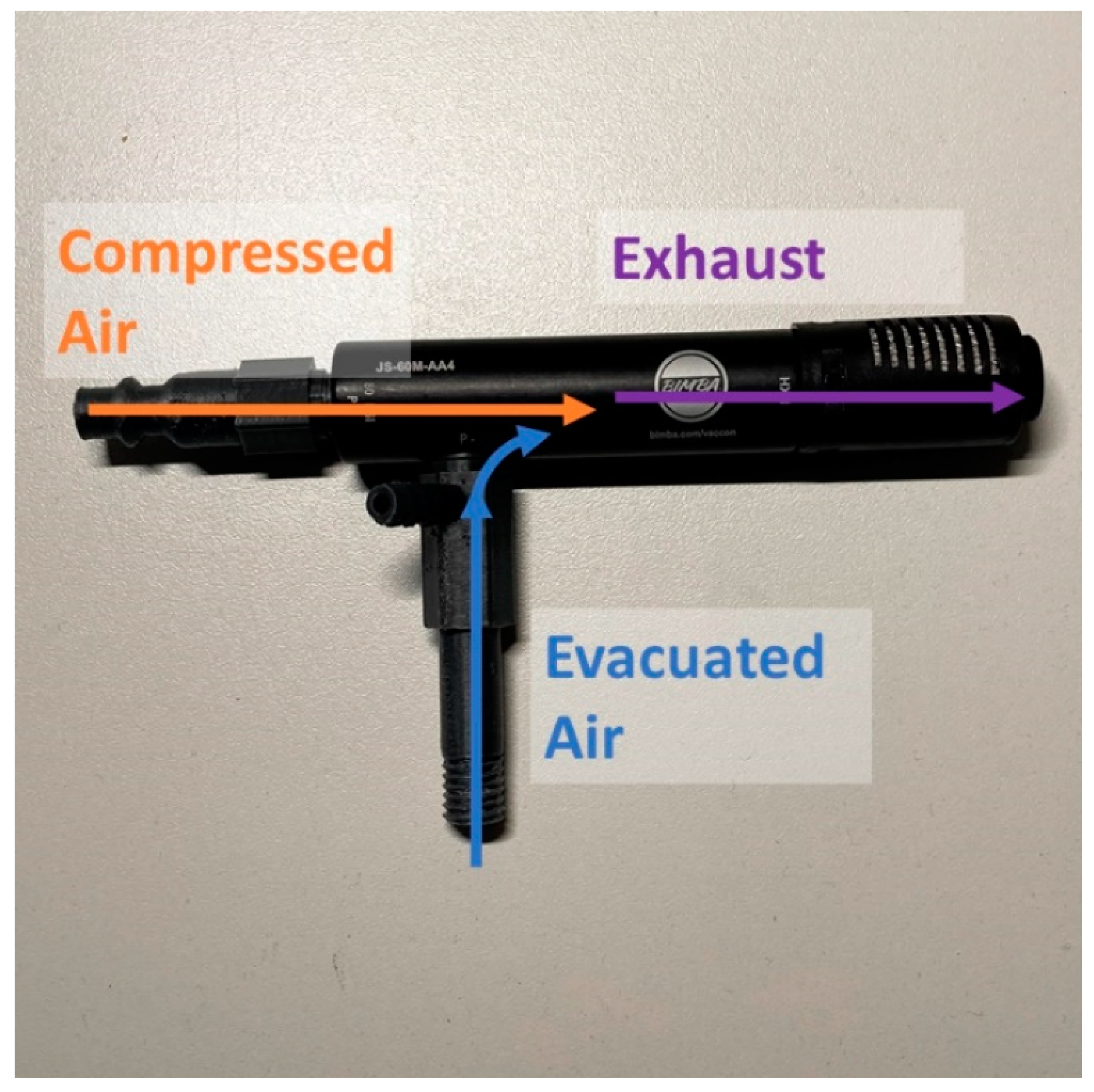
2.1.1. Vacuum System

The physical vacuum chamber selected was an off-the-shelf vacuum chamber, measuring 200 mm in diameter and 200 mm in height, which was designed to handle vacuum pressures up to 98 kPa (29 inHg) [27]. This is a sufficiently deep vacuum to allow drying at or only slightly above room temperature [28]. Vacuum pressure (the difference between evacuated pressure and atmospheric pressure) is a convenient metric for discussing the mechanical behavior of the chamber and the vacuum pump, as their performance is directly linked to vacuum pressure—in how much pressure the chamber can withstand, and how deep a vacuum the pump can draw. However, the thermodynamic behavior of water depends on the absolute pressure of the atmosphere in which the water is present. Since atmospheric pressure varies with elevation and weather, the vacuum pressure required to reach a certain absolute pressure can vary. This can be confusing when looking at the performance of a vacuum oven. To help distinguish between these two quantities, they will be expressed in different units following the protocol for water saturation tables [29]. Vacuum pressure will be noted in inHg, where 0 inHg is atmospheric pressure at sea level, and 29.9 inHg is an absolute vacuum. Absolute pressure will be noted in kPa, where 0 kPa is an absolute vacuum, and 101.3 kPa is atmospheric pressure at sea level. Finally, gauge pressure, and pressure measured above atmospheric pressure will be expressed in psig (pounds-per-square-inch-gauge). Each set of units was selected directly from the instrument or reference material providing the relevant measurement. The vacuum gauge provides inHg [30], thermodynamic tables [28] and a list saturation points of water with absolute pressure in kPa, and the air compressor measures output pressure in psig [31]. All values are also denoted in kPa, with the reference noted as ‘absolute’, ‘vacuum’, or ‘gauge’.
An air ejector was selected to act as the vacuum pump for this system and details of the selection process are provided in Appendix A. Air ejectors (also called venturi ejectors, venturi vacuums, air-powered vacuum pumps, and air-jet ejectors) use high-pressure air and a combination of converging–diverging nozzles to create vacuum pressure [32,33,34]. The shape and size of the nozzles can be varied to affect the required inlet pressure, the rate of evacuation, the depth of vacuum, and the volume of air consumed by the ejector [33,35]. The practical limit of a single-stage air ejector is an absolute pressure of around 6.7 kPa [34], which brings the saturation temperature of water just below 40 °C [28]. Other methods can achieve a deeper vacuum, but this allows for a sufficiently low temperature to encourage rapid evaporation. In addition, an air ejector has the advantage of being driven by compressed air. Since air is being forced through the ejector and out into the atmosphere, never moving through a machine, there is no risk of damage to equipment due to water or other materials which may get caught up in the flow of evacuated air [36]. On an industrial scale, compressed air is often already present in other processes, mitigating the cost of introducing a vacuum system [36]. Similarly, in small labs or distributed fablabs and makerspaces, an air compressor is much more likely to be a part of the existing toolset (and more generally useful) than a mechanical vacuum pump. Air ejectors are commercially available at a similar cost to vacuum pumps [37]. Due to the robustness and cost effectiveness of an air-ejector, this was selected to evacuate the chamber.

2.1.2. Thermal Controls

The thermal control system is composed of a heater, controlled by a relay and a micro-controller. The micro-controller measures the temperature of the heater pad with a negative-temperature-coefficient (NTC) thermistor. A thermistor is a sensor whose resistance varies as a function of temperature. They are commonly used in 3-D printing and offers a measurement precision in the order of 0.2 °C, though the accuracy depends heavily on the accuracy of the model used to calculate temperature, the temperature range being measured, and the resolution of the analog-to-digital converter (ADC) used to measure the thermistor [38,39]. The resistance of the thermistor was measured by an open source Arduino microcontroller [40] using a voltage divider with a known reference voltage and resistance. The measured resistance was used to estimate the temperature (and vice versa) using what is known as the Steinhart–Hart Equation [41], which characterizes a thermistor based on three resistance values, measured at three known temperatures. This model tends to be accurate within half a degree Celsius over the calibration range [41] but is often simplified to a two-point model, which requires a single coefficient, the Beta coefficient, and is simpler to calibrate and compute while measuring. This simplified model maintains a similar accuracy over a smaller temperature range [39,42,43]. The simplified Steinhart–Hart Equation was used for measuring the temperature of the heating element.
The challenge of building a robust thermal control system for a vacuum oven is significant, particularly with the use of off-the-shelf parts. The primary mode of heat transfer inside the vacuum chamber is conduction, which cannot be accurately modeled for the design of a controller, as it depends on many factors including the type, volume, density, and surface area of the material inside, as well as the rate of heat loss to the environment. In order to control the temperature inside the chamber without damaging the chamber, the approach selected was to track the temperature of the heating element—a flexible silicone heating element measuring 100 mm by 125 mm, used as engine block heaters or 3-D printer bed heaters. These offer a large surface area and relatively low power per unit surface area (Watt density), which is preferable for low set temperatures, since it reduces the rate at which the heater must switch on and off to maintain a set temperature [44]. The controller operates on the assumption that sufficient insulation and time allow the inside of the vacuum chamber to reach equilibrium at or near the temperature of the heating element. In order to quantify the inevitable temperature difference between the heater and the inside of the chamber, the gradient was measured with loosely packed rPET in the chamber. These measurements were used to inform set temperatures for the oven during testing that manually correct for the temperature difference. It was found, from the perspective of drying speed, that this approach is applicable on small samples (tens of grams). In order to control the temperature of the heater, a simple relay control system was used. This was selected because the thick metal of the chamber sufficiently filters out the switching effects of the relay, providing a smooth temperature curve inside the chamber.

2.2. Manufacturing and Assembly

The vacuum consists of 3-D printed and off-the-shelf parts [27,30,31,37,45,46,47,48,49,50,51,52,53,54,55,56,57]. The parts can be seen in a visual Bill of Materials (BOM) in Appendix B.

2.2.1. Vacuum Chamber

To prepare the vacuum chamber for assembly, two strips of Reflectix insulation were cut about 5 cm wide and 2–3 times the circumference of the chamber in length. These were used to build an air-gap between the Reflectix and the sides of the chamber, per Reflectix’s installation recommendations [58]. They also helped the bulk insulation span over handles and clasps protruding from the wall of the chamber. Another piece of Reflectix insulation was cut with the same length (2–3 times the circumference of the chamber) and as wide as the chamber is tall. This was used to insulate the sides of the chamber. Finally, four circles of Reflectix of the same diameter as the lid of the chamber were cut to insulate the top and bottom of the chamber. Two of the circles were set on the lid, and a slit was cut in both layers over the hole in the lid. The vacuum inlet of the air ejector feeds through this slit. A thin strip and the circles of insulation are shown in Figure 1.
Next, the air ejector was assembled. The selected air ejector has 1/8-inch National Pipe Tapered (NPT) female threads for the air intake and vacuum inlet. The air intake must connect to an air compressor hose, which has a ¼-inch I/M coupler (often called a quick-connect). The vacuum inlet must connect to the chamber lid and a vacuum gauge. On the vacuum chamber in use, the lid was sized for an M10 vented bolt. The selected vacuum gauge required a 5 mm hose barb. Rather than purchase and plumb together, several connectors to accomplish this, the connectors were 3-D printed. The internal geometry of the printed connectors is shown in Figure 2. To create the composite parts, the hose barb and I/M coupler were modeled in FreeCAD v0.18 [59] based on measurements of purchased parts. FreeCAD offers straightforward profile-modeling tools, but OpenSCAD [60] has a broader, more robust set of thread libraries, so OpenSCAD v2019.05 was used to compose the final parts. Kirshner’s ‘threads’ library [61], available under the GNU GPL 3.0 [62], was used to create ISO-standard metric threads for the M10 nut. Corona688′s ‘tmsthread4′ library [63], available under the Creative Commons Attribution Non-Commercial (CC-BY-NC) license [64], was used to create NPT threads for both components.
The design and STL files for each component are available, along with all other data, designs, and documentation, on the OSF repository [45] under the GNU General Public License (GPL) 3.0 [62]. Note that the 3-D printed parts are available under CC-BY-NC [64] because they use tmsthread4 for the NPT threads. All other files and data are available under GPL 3.0. The original CAD files (OpenSCAD [60] and FreeCAD [59]) are available to allow modifications in the case that the parts they attach to are different than those used in this build. The components were 3-D printed using a 1.75 mm polylactic acid (PLA) filament on an Athena II delta-style RepRap class 3-D printer [65] with a 0.4 mm nozzle. The STL for each component was sliced using Ultimaker Cura v.4.7.1 [66] and the print settings were shown in Table 1. After printing, supports and brim materials were cleaned off the prints.
Testing has shown that the printed parts can withstand the high pressure (550 kPa gauge, or 80 psig) at the intake and low pressure (88 kPa, or 26 inHg vacuum) at the vacuum inlet, and the printed threads work and properly seal at the connections. The connectors were threaded into their respective sockets on the air ejector (Figure 3a). To check that the ejector was functional, the vacuum gauge was attached (Figure 3b) and a 550 kPa (80 psig) gauge pressure air was applied to the air intake. Plugging the vacuum connector showed around 80–86 kPa (24–26 inHg) vacuum pressure on the gauge. To resolve issues with a faulty seal on the connectors, adding a polytetrafluoroethylene (PTFE) thread seal tape can help—note that PTFE tape is only intended for tapered threads [67], so it will not help with the M10 threads. Airflow through the assembled air ejector is shown in Figure 4.
With the air ejector assembled and checked, the vacuum inlet was fed through the two circles of insulation. Next, one M10 washer was placed on the inlet (Figure 5a), then the inlet was fed through the lid of the vacuum chamber. The other M10 washer was applied and the M10 nut was tightened onto the threads, securing the air ejector and insulation to the lid (Figure 5b).
Finally, the insulation was installed on the walls of the chamber. This was done after installing the heating element, allowing the sensor wire and power cable to be fed through the wall insulation (as shown in Figure 6) for strain relief.
To install the wall insulation, the two strips of insulation were wrapped around the top and bottom as shown in Figure 7a, securing them to the chamber wall and themselves with flue tape (other adhesives may be used if lower temperatures will be used for drying). Next, the large strip of insulation was wrapped around the walls of the chamber, once again using tape to secure it to the already installed layers of insulation, and to itself. The final result is shown in Figure 7b.
The two layers of insulation for the base of the chamber were installed after the installation of the heating element.

2.2.2. Thermal Control System

Before building the thermal controller, thermistor calibration measurements were collected to calculate the Beta coefficient of the thermistor. The thermistor’s resistance was measured at 0 and 100 °C by submerging the thermistor in an ice bath and boiling water, respectively. The thermistor was wrapped in flue tape prior to submersion to protect it from short-circuiting in the water. The resistance measurements were recorded and used to calibrate the thermistor as described in Section 2.6.1.
The controller measures the thermistor with a voltage divider, which uses a reference resistance connected to the reference voltage. This resistance is placed in series with the thermistor, which is connected to the ground. The voltage at the node connecting the two resistances is measured with an analog pin on the Arduino. This voltage is used to determine the resistance of the thermistor. The value of the reference resistance has a direct impact on the precision of the temperature measurement. Increasing the difference between the measured voltage at the upper and lower temperature bounds increases the number of discrete voltages (therefore, temperatures) that the ADC can measure. The measured voltage, Vm, for a given voltage divider with a thermistor resistance (Rth) and reference resistance (R0) is calculated using Equation (1). This equation assumes that the reference voltage is 1 V, meaning that the difference between two measured voltages corresponds to a percentage of an ADC’s measurement range.
Vm = Rth/(R0 + Rth)
The difference between Vm at the upper (Rth1) and lower (Rth0) operating resistances should be maximized. Using the simplified Steinhart–Hart equation (Equation (2)), the thermistor resistance was estimated at the upper and lower operating temperatures. The nominal resistance and temperature, 100 kOhm at 25 °C, were used as R1 and T1, respectively. The nominal Beta value, β, provided by the manufacturer, 3950, was also used [50]. A calibrated value could be used instead, after completing the thermistor calibration as described in Section 2.6.1.
β = ln(R1/R2)/(1/T1 − 1/T2)
With these values estimated, selecting R0 became a simple optimization problem, with the cost function (Cf) in Equation (3). The equation is written in such a manner to emphasize that the difference between the two measured voltages should be maximized, making no assumptions about which voltage will be larger. The sign is changed because optimization conventionally seeks to minimize cost.
Cf = −abs(Rth0/(Rth0 + R0) − Rth1/(Rth1 + R0))
This cost function was minimized using ‘minimize_scalar’, which is an optimization method in the SciPy Python library’s ‘optimize’ package [68]. Intuition would suggest that the optimal resistance R0 has a magnitude on the order of the thermistor resistance, so the initial guess provided to ‘minimize_scalar’ was the average of the operating bounds. A Python script named ‘voltage_divider_optimization.py’, which returns the optimal resistance, is available on the OSF repository [45]. It accepts the thermistor beta value and references the temperature-resistance pair, plus the operating temperature range, completing all other computations internally.
The optimization was run for a few operating ranges, shown in Table 2. The operating range during design was expected to be 50 to 60 °C, so a 30 kOhm resistor was used. A similar approach to this problem, as well as a further explanation on the rationale, have been discussed by Hrisko [69].
The thermal control circuit, shown in Figure 8, is fairly simple—it only requires a voltage divider, used to measure the thermistor resistance, and a pair of signal wires to control the relay.
The circuit was assembled on a 3 × 7 cm solder breadboard. The assembly of that board is detailed in Appendix C, and the final circuit is shown in Figure 9.
With the circuit fully constructed, the dryer firmware (available on the OSF repository [45]) was uploaded to an Arduino Nano, which was then installed in the female header pins with the USB on the column ‘A’ side of the board (Figure 10a). The thermistor was attached to its male header pins and the relay was connected to the signal wires (Figure 10b).
The heating pad had an adhesive on one side. The transfer tape was removed from the heating pad, revealing the adhesive. Prior to installing the heater on the base of the vacuum chamber, the thermistor bulb was stuck to the middle of the heating pad. Adhering the pad to the base of the chamber secured the thermistor in place (Figure 11), providing a direct measurement of the heater temperature. Pressure was applied to the heating pad for 60 s to allow the adhesive to set.
To allow the heater to be controlled by the relay, the heater power cable was cut in half (Figure 12a). Only one wire needs to be severed—the other can remain intact. In this case, both wires were cut, so one pair of wires was re-connected using a wire nut (Figure 12b).
The other pair of wire ends were stripped and secured in the load terminals (1 and 2) of the relay, as shown in Figure 13.

2.2.3. Finishing the Assembly

In an effort to tidy the wires and make transportation easier, the electronics for the oven were assembled on a wooden frame. The relay was secured with two M4 machine screws, and the circuit was secured with four M2 machine screws. Power was provided to the Arduino and the heater via a power strip, also attached to the board. The final assembly is shown in Figure 14.

2.3. Code

The firmware driving the dryer is straightforward. It uses Salimov’s NTC_Thermistor library to handle the simplified Steinhart–Hart equation for computing the temperature from the voltage divider measurement [70]. The temperature measurements are read into a 10-sample averaging finite impulse response (FIR) filter. A longer average could feasibly be used without affecting the dynamics of the system, but this number of averages is memory-efficient for the Arduino and was found to be sufficiently smooth for the purposes of control.
The system tracks the average temperature and uses relay control with no hysteresis to regulate the heater temperature—turning the heater on if the temperature is below the set temperature, and off if it is above. Testing showed that the switching of this relay was sufficiently filtered out inside the chamber, making a more sophisticated controller unnecessary.
Every second, the current time and temperature are printed to serial for the sake of data logging and checking performance. In an effort to prevent catastrophic failure due to a sensor error, the temperature is checked to make sure it is reasonable. In the event that the thermistor open-circuits, the resistance reading should fall to around absolute zero (−273.15 K). Designing on the assumption that the vacuum oven will not be used in a room where the temperature is below 0 °C, a temperature reading below 0 will force the relay to turn off and throw a message over serial that something is wrong. This value can be changed to meet different needs, or even to track a predictive model to further improve failure-safety. In the opposite event, should the thermistor short-circuit, the controller would read a very high temperature, above the set temperature for the heater, so the relay would naturally turn off.

2.4. Operation

Operation of the oven requires a few steps. First, the material to be dried was placed in the oven. Next, the operating temperature was set to meet the limits of the material being dried. The upper limit for a safe operating temperature is two-fold. First, the heating element comes with a thermal fuse set to trip at around 130 °C, meaning that temperature cannot be exceeded. Secondly, the chamber lid is made of acrylic and the manufacturer recommends that it not be exposed to temperatures greater than 60 °C [27]. With the current design, the temperature gradient on the chamber is significant, making the lid little cause for concern. Improvements to the design which provides a more even heating of the chamber must take this into consideration. The current firmware uses a hard-coded set temperature. This value was changed by editing the variable T_set in the firmware, then re-flashing the Arduino. This removed any need for a user interface (such as a display to show, or knobs to vary, the set temperature), though one could be added in the future. Once the temperature was set, the heating element was turned on by providing power to the Arduino and the heater.
With the material loaded and warming up, the only remaining step was to introduce a vacuum. First, the lid was placed on the chamber, and the air compressor hose connected to the compressor and the lid. The manufacturer recommends that this be completed prior to charging the air compressor for safety [31]. Next, the air compressor was turned on and allowed to charge to full capacity. Once the pump had turned off, the pressure regulator was set to provide 550 kPa (80 psig) gauge pressure to the air ejector. Light pressure was applied to the lid until the vacuum gauge started to show a vacuum pressure. At this point, the lid was held in place by air pressure. The ultimate vacuum achieved was around 84 kPa vacuum (25 inHg), or about 17 kPa absolute. At this pressure, the saturation temperature of water is approximately 57 °C [28].
The testing discussed in the results offer some guideline for the amount of time required to dry material, but testing should be conducted to determine the appropriate time and temperature for drying specific materials. The test procedure used here offers a framework for determining such drying times.

2.5. Materials for Testing

The system was tested with both plastics for DRAM and biomaterials as part of a project to convert post-consumer plastic into edible food.

2.5.1. Plastics

rPET, which is the most abundant waste plastic, was produced for testing by washing and shredding used water bottles into flakes. PET is a highly hygroscopic material, meaning it tends to absorb water into its chemical structure [5,71]. Absorbed moisture can only be removed to the point of equilibrium with the air surrounding the material. This means that simple hot-air drying cannot make the plastic any dryer than the air in the room. This can be a major impediment to the successful use of rPET in DRAM as for example simple air drying does not work in humid environments. Thus, converting rPET to 3-D printing filament is normally regulated to demonstrations on lab-grade or industrial grade recycling systems using blends [72,73] or composites [74] rather than low-cost open source recyclebots (waste plastic extruders that produce filament) [75,76], which are more appropriate for DRAM. Vacuum drying offers a much lower atmospheric moisture content than hot-air drying, meaning that it can dry hygroscopic materials more completely than hot-air drying [71]. The rPET offered an opportunity to check for signs of this behavior, limited by the measurement resolution of the balance in use. Prior to testing, the rPET was placed in an unsealed container for a span of several days to provide an opportunity for the plastic to reach an equilibrium of moisture content with the laboratory air.

2.5.2. Biomaterials

Another approach to recycling PET is to use bio-organisms to convert it to useful products like food. To begin to probe this potential, microorganisms were grown on rPET chemical components. Specifically, terephthalic acid is a building block of polyester plastics such as PET. Various bacteria can use terephthalate as a carbon and energy source [77,78]. A bacterial consortium was enriched from compost with the ability to grow to high densities using terephthalate as a sole carbon source. This consortium shows promise for the bioprocessing of terephthalate wastes, as well as potential transformations of plastics like PET.
Single cell protein (SCP) is protein that is derived from single-celled organisms such as bacteria and algae [79]. SCP has been proposed as an alternative food source to deal with growing food insecurity [80,81]. To convert microbial biomass into single cell protein, biomass needs to be treated to both preserve and inactivate the cells. Here the novel drying system is tested as a post-treatment procedure to generate SCP from microbial biomass grown on terephthalate.
Enrichment cultures were set up using a sample of vermicompost, which is a compost that is broken down using worms, from a farm in Calumet, MI, USA (47.211, −88.553). The vermicompost was sampled using a pre-sterilized scoop and was collected in a sterile 50 mL Falcon tube. The sample was placed on ice and transported back to Michigan Technological University, where it was stored at 4 °C.
Aerobic cultures were set up in sterile 250 mL Erlenmeyer flasks using 1 g of vermicompost soil, 100 mL of Bushnell-Haas media (0.2 g/L MgSO4, 0.02 g/L CaCl2, 1 g/L KH₂PO₄, 1 g/L (NH₄)₃PO₄, 1 g/L KNO3, 0.05 g/L FeCl3), 0.25 g terephthalic acid, 0.25 g terephthalamide, 2.5 mL of chemically deconstructed polycarbonate product, and 0.125 mL of a 1:1:1:1 mixture of C6:C10:C16:C20 alkenes. The deconstructed polycarbonate product served as a source of bisphenol A. Cultures were placed in a temperature-controlled shaker and incubated at 200 rpm and 30 °C. Cultures were transferred into fresh media of the same composition at a 1:10 dilution once every two weeks. After five transfers, 100 µL of material from the enrichment cultures were transferred for growth on disodium terephthalate for biomass production. The consortia were transferred four times in Bushnell Haas medium with 10 g/L disodium terephthalate as the carbon source prior to the growth of the consortia for biomass production as described below.
To produce biomass for the dryer, 500 mL of Bushnell-Haas medium supplemented with 10 g/L of disodium terephthalate was inoculated with 5 mL of the culture grown on disodium terephthalate and incubated at 25 °C for three days. Biomass from the consortium was harvested by centrifugation at 7500× g for 10 min. The supernatant was removed, and the biomass was stored at 4 °C until use for testing the open source vacuum oven in drying.

2.6. Testing

2.6.1. Thermistor Calibration

The thermistor was calibrated using resistance measurements gathered at three known temperatures, shown in Table 3. These measurements were used to calibrate the full Steinhart–Hart Equation (Equation (4)), which has three coefficients and is solved with a system of three equations as previously described [41].
T = 1.0/(ka + kb*log(Rt) + kc*log(Rt)3)
Three combinations of the measurements in Table 3 were then used to compute Beta three times. The thermistor curves for those three Beta values, plus the nominal value, were compared with the full Steinhart–Hart Equation. These computations were completed using a Python script named ‘thermistor_calibration.py’, available on the OSF repository [45]. The Beta value that provided the least error was selected to calculate temperature on the Arduino.

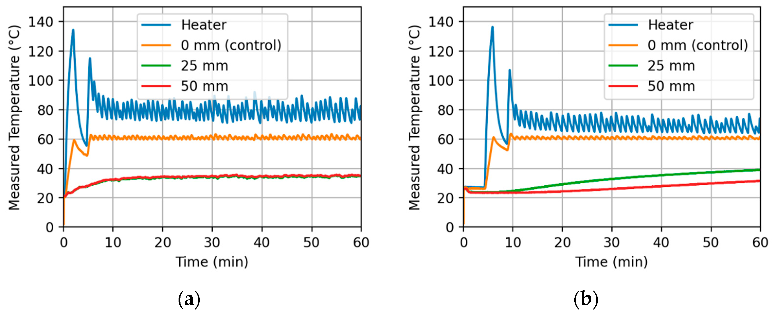
2.6.2. Temperature Gradient Measurements

In order to quantify the temperature gradient resulting from the location of the control temperature sensor, three thermistors were installed on a 3-D printed jig in the center of the chamber. The jig held the thermistors 0, 25, and 50 mm above the base of the chamber. The thermistor jig is shown in the chamber in Figure 15a. These temperatures were measured on a separate microcontroller from that driving the heater. The measurements were taken with rPET material inside the chamber, with the chamber at atmospheric pressure (measuring the temperature under vacuum conditions faced the same challenges as for placing the control thermistor inside) and the lid off. The thermal controller was set to 60 °C, measured at the heating element. This test was completed twice: (1) with only rPET inside the chamber; then (2) with an added metal cylinder (referred to as a heat sink) inside to aid in the distribution of heat to the rPET. The heat sink with the thermistors and rPET is shown in Figure 15b.
An additional set of tests was completed in which the thermistor mounted at 0 mm (on the base, inside the chamber) was used to drive the relay controller. This was tested with no material in the chamber, and with rPET in the chamber. Once again, the lid was off, meaning the thermistor was exposed to convective interference that would otherwise not be present under vacuum. The temperatures of the heater and the 25- and 50-mm thermistors were recorded. This configuration offered an approximation of how the controller would behave if the control thermistor were mounted inside the chamber while under vacuum. The results indicated the necessary heater temperature to reach an inside surface temperature of 60 °C, and aid in estimating the inside surface temperature for a given heater set temperature.

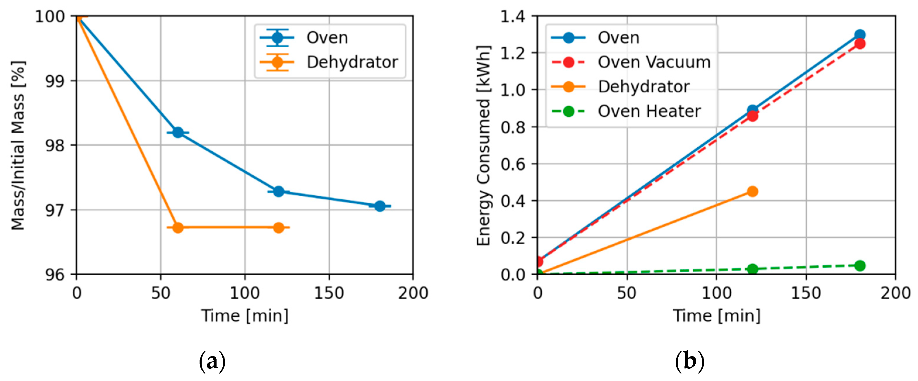
2.6.3. Drying Rate Comparison

The vacuum oven was tested against an off-the-shelf food dehydrator [82], which would be classified as a typical hot-air dryer. To quantify the dehydration of each sample, the mass of each sample was measured prior to and throughout testing using an open-source precision mass balance, calibrated using a 100 g standard mass with a rated precision of 5 mg [26]. The mass measurements were taken external to each drier, at atmospheric pressure and temperature. During each test, the energy consumption of the vacuum oven and the food dehydrator were each measured using multimeters, measuring energy in kWh to 0.01 kWh precision [83]. The vacuum oven’s heating and vacuum (air compressor) energy consumption were measured separately to help identify where the majority of energy consumption occurs.
Testing was first conducted on small samples (10 g) of rPET to determine a set temperature for the oven. The samples were measured on a 100 g load cell with a reported measurement accuracy (standard deviation) of 5 mg [26]. Three 10 g samples were prepared in petri dishes with known masses and 300 mg of water was added to each sample, bringing the total mass to 10.3 g, such that the added water comprised approximately 3% of the mass. The first sample was placed in the center of the vacuum oven base, which was set to 70 °C. The second was placed on the lowest shelf of the food dehydrator, also set to 70 °C (its maximum temperature). All trays provided with the dehydrator were left in the assembly during testing, in accordance with the operating instructions [82]. The third sample was left on a counter to act as a control. Every 15 min, each sample was weighed while left in its petri dish. This ensured that no flakes of plastic or droplets of moisture could be left behind in transfer between containers. The mass of the empty petri dish was subtracted from the measured mass, recording only the mass of the plastic and water. This was repeated with the vacuum oven set to 80 °C.
Next, large samples (350 g) of rPET were tested with the vacuum oven set to 80 °C. At this point, small sample testing had showed that both dryers acted faster than a control, so no control was kept for further measurements. Each large sample was measured on a 5 kg load cell with a reported measurement accuracy (standard deviation) of 20 mg [26]. The samples once again had 3% water by mass added, constituting 10.8 g of water. Given the size of the sample, the plastic was stirred after the addition of water to encourage an even distribution of water throughout the sample. These samples were too large to keep in containers within each dryer, so measurements were made less often (every 60 min), and the plastic was transferred from each dryer to a separate bowl for each measurement. In the vacuum chamber, two metal cylinders were included as heat sinks during the large sample tests. In the dehydrator, all trays were filled with plastic. The lowest tray had a dense metal screen of material installed to minimize the loss of small pieces of plastic into the base of the dehydrator.
To test the drying of biomass, samples of approximately 500 mg were measured into petri dishes, once again with the mass of the container measured beforehand. The biomass was expected to be about 60% water by mass, so no water was added. These samples were measured every 15 min while being dried.
The results of the drying tests are shown as a computed value—the percentage of the initial mass (pim) remaining at each measurement, calculated using Equation (5), where mi is the initial mass and mm is the measured mass. This serves two purposes. First, it corrects for any differences in initial mass between each sample, thus correcting out vertical offsets in the data. Second, it highlights the percentage of mass lost in terms of the percentage moisture content. The rPET tests each had 3% water by mass added to the sample prior to testing, and every sample (except for the large vacuum oven sample, which was cut short) showed a reduction in mass to below the initial ‘dry’ mass, indicating that additional pre-existing moisture was removed from the plastic during drying. Since each curve is scaled to a percentage mass, error bars are included to indicate uncertainty (me) in the mass measurement. The error is shown as a percentage of the measured mass (pmm), calculated in Equation (6), and hence smaller masses have a larger percentage of uncertainty, because they approach the magnitude of the measurement error of the load cell.
pim = mm/mi [%]
pmm = me/mi [%]

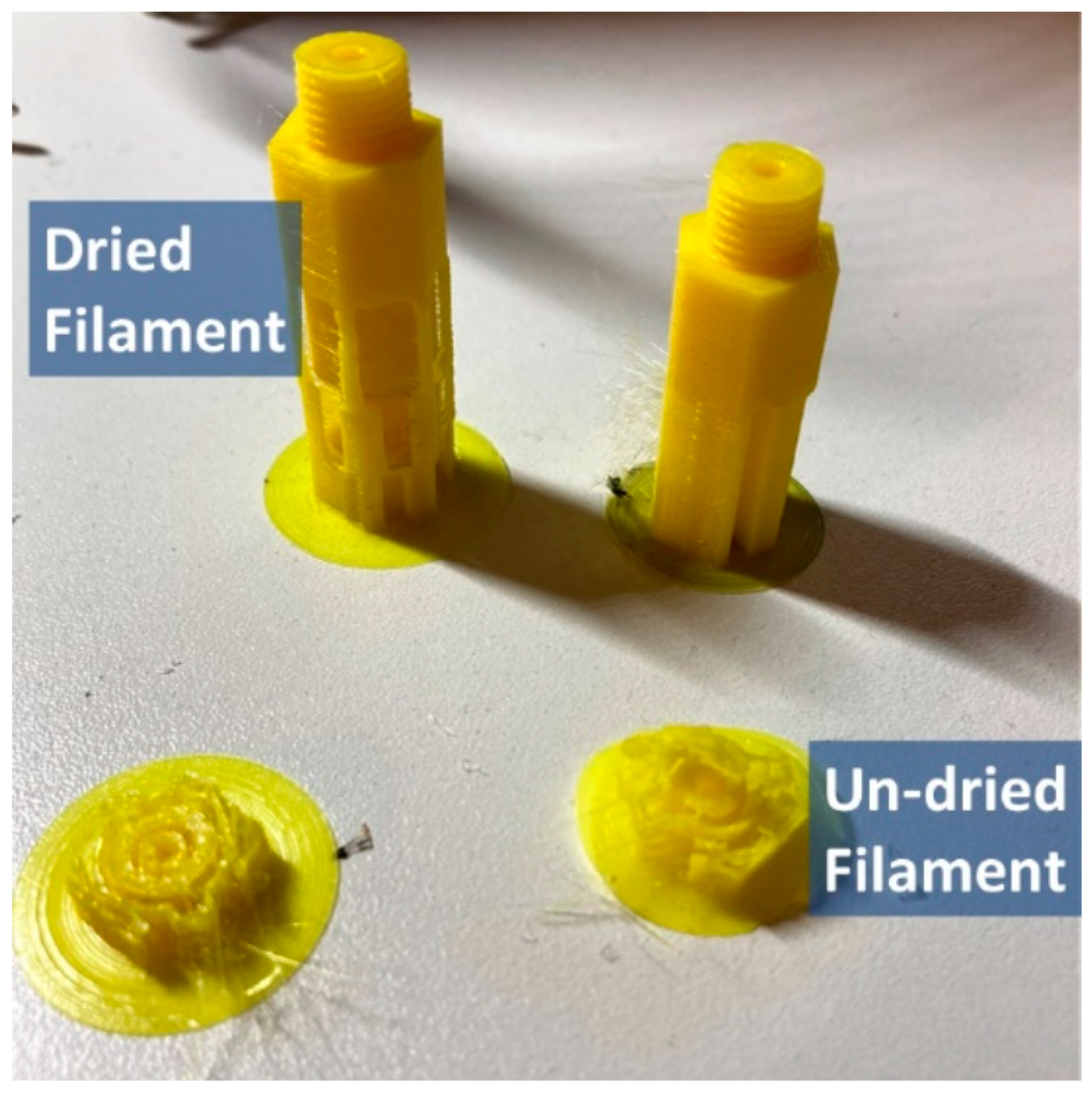
2.6.4. Filament Drying

To verify the effects of the vacuum oven on Fused Filament Fabrication (FFF) 3-D print quality, two tests were run. First, two small (~30 g) samples of PLA filament were taken from a single spool of PLA filament, which had been stored in a humid environment. The first sample was used to print the vacuum connectors from Table A1. The second sample was dried using the printer, set to 60 °C, for two hours, then used to print the same parts. Both prints were completed on the same day and with the same printer. The resulting prints were photographed for visual comparison.
Second, a 1 kg spool of PLA filament, which had been stored in a laboratory, was dried in the vacuum oven, set to 80 °C. The mass of the spool was measured every half hour until no changes in mass were observed. This mass was measured using the same 5 kg load cell as was used for the large samples of rPET.

2.7. Economic Analysis

To quantify the cost of this device, its total cost is divided between the two components. Here only the material costs are considered. Several components are available for bulk purchase, providing enough material for multiple builds of this device, or use on other devices. This means that the device has two costs. First, the up-front cost, that which would be paid to build a single vacuum oven, counting all leftover material as cost for the build. This is the summation of the bulk price, Pb, of each component. Second, the effective cost, Ce, which accounts for only the material used in the build. This is computed by Equation (7), which corrects the bulk price using the bulk volume, Vb, and the volume consumed, Vc. The computation of the bulk and effective cost is completed in the BOM spreadsheet, available on the OSF repository [45].
Ce = Pb × Vc/Vb
where the correction is applied to each component’s cost. The cost of 3-D printed materials (listed in Table A1) is the mass of the part times the cost of plastic per kg. The cost of the PLA filament for the Athena II was U.S. $19/kg [84].

3. Results

3.1. Thermistor Calibration

The calculated full-model coefficients for the Steinhart–Hart Equation are shown in Table 4.
These were used to compute the thermistor curve shown in Figure 16.
The computed Beta values are shown in Table 5. These were used to generate comparison curves with the full model. The difference between the full and simplified model for each Beta value is shown in Figure 17. The calibration shows that a Beta equal to 3920 or 3950 is the best option, maintaining an error within 1 °C for the expected operating range. Since 3950 is the nominal value, it was used in recognition of the potential error in measuring the resistance and the actual temperature of the thermistor during the calibration measurements.

3.2. Temperature Gradient Testing

The measured temperature gradient in the chamber with and without an added heat sink is shown in Figure 18. The three thermistors show a very steep gradient and a slow rise for the temperature in the chamber. The measurements indicate that a heat sink amidst the loosely packed material greatly increases the rate of warming throughout the chamber.
The measured temperature gradients while using the inside (0 mm) thermistor to drive the controller are shown in Figure 19. With no material in the chamber, the heater had to maintain an average temperature of 79 °C to keep the inside surface of the chamber at 60 °C. Note that the chamber was open to atmospheric air, allowing convective heat loss. After the addition of rPET (still at atmospheric pressure), the heater temperature averaged around 68 °C in order to maintain an inside surface temperature of 60 °C. Note here that the PET had not reached a steady state temperature after one hour of testing. The gradient is likely exacerbated under vacuum conditions because convective heat transfer is no longer possible, restricting heat transfer only to conduction. These results suggest that a set temperature of 70 to 80 °C on the heater should yield an oven temperature (only at the inside surface of the base) of 60 °C (slightly above the saturation temperature of water at the measured vacuum pressure). The addition of bulk material to the oven slows the transfer of heat upward through the chamber, apparently by reducing the rate of convective loss. This observation highlights two possibilities. First, introducing a vacuum will virtually eliminate convective loss inside the chamber, meaning the temperature gradient between the heater and the inside surface of the chamber should be small; and, second, the bulk material acts as insulation, meaning heat transfer in the absence of convection will likely be slow, resulting in a significant temperature gradient on large samples under vacuum. This temperature gradient is likely to negatively affect the rate of drying as the top layer of large samples will not reach the saturation temperature of water.

3.3. Drying Tests

During all drying tests, the ultimate vacuum achieved in the vacuum oven was approximately 84 kPa vacuum (25 inHg), or 17 kPa absolute, which reduced the saturation temperature of water to around 57 °C. The results of small sample tests are shown in Figure 20. At 70 °C, the sample in the vacuum oven was considered dry after 75 min, and the dehydrator sample was considered dry after 60 min, making the vacuum oven 25% slower than the dehydrator at this setting. This corresponds with what was expected from the temperature gradient tests—a set temperature of 70 °C may not have brought the inside of the chamber up to the saturation temperature of water, limiting the rate of evaporation. Increasing to 80 °C ensured that the samples were warm enough to cause rapid drying. In this case, the vacuum oven sample was dried after 45 min, while the dehydrator (still set to 70 °C) took 75 min, making the oven 40% faster in this test, and 25% faster than the dehydrator on either 10 g sample tested. The increased set temperature caused a significant improvement in the oven’s performance, even though gradient testing suggests it is likely that the material in the oven was still at a lower temperature than the dehydrator. The dehydrator settings were not changed between these two tests, yet they show a significant variation between the two tests. This variation was accepted as the variation in real-world conditions for the dehydrator and were not explored in testing. In both cases, the energy consumption of the dehydrator over the span of the 90-min test was about 0.36 kWh. The vacuum oven consumed 0.61 (Figure 20b) and 0.55 kWh (Figure 20d), respectively. The difference between these is directly related to the number of times the air compressor cycled to refill its tank. The energy required to fill the compressor tank from empty was included in the total energy on the first test only, accounting for 0.04 kWh of the difference in total energy consumed. These results show that the vacuum oven consumes about 70% more energy than the dehydrator for a given amount of time.
The results of the large sample rPET test are shown in Figure 21. The immediate conclusion drawn from this test was that the vacuum oven cannot handle large volumes of water. During the test, condensation was observed on the lid and upper wall of the vacuum chamber. Condensation indicates that the lower portion of the oven was heating sufficiently to evaporate moisture, but the top of the oven was cool enough to allow water to re-condense before being evacuated from the chamber. Given time, the trend shows that the oven could remove all the present moisture. The food dehydrator, however, proved to be significantly faster when drying large samples. The energy measurements for this test are shown in Figure 21b. The energy data, consistent with other results, show that the vacuum oven consumes about twice as much energy as the food dehydrator with a vast majority (96%) of the energy going to the air compressor to maintain vacuum pressure in the chamber.
Further testing of oven drying efficiency was performed on small samples of microbial biomass. The 500 mL culture grown on disodium terephthalate produced 2 g of biomass by wet weight after three days of growth. Approximately 1 g of biomass was dried, with 500 mg tested in each dryer. The culture is shown before and after dehydration in Figure 22.
The results of using the open source vacuum oven for biomass dehydration on these samples are shown in Figure 23. These results show the vacuum oven dehydrating the biomass at a much higher rate than the food dehydrator. The oven settled out in about 75 min, while the dehydrator took 150 min. The small masses (around 500 mg) under test likely contributed to the performance of the vacuum oven. The small sample sizes also result in larger measurement uncertainty from the reported accuracy of the load cell, as indicated by the error bars. The observed difference in the final percent of initial mass is expected to be a result of the biomass sample being non-homogeneous. After completion of the test, the sample from the dehydrator was moved to the vacuum oven to check if it could remove more moisture than the dehydrator had. No additional loss of mass was measured after 15 min, meaning there is no evidence to suggest that the vacuum oven dried the biomass more completely than the dehydrator.
These test results are summarized in Table 6. This includes an average specific energy consumption value, calculated by dividing the total energy consumed by the total mass removed. They show that the vacuum oven is more efficient than the food dehydrator (with regard to time and energy) for small samples when the set temperature is 80 °C. The dehydrator proved to be more efficient when handling larger masses of water due to the uneven heating in the chamber. The average specific energy consumption shows that both devices become significantly more efficient when drying larger samples. This happens because the material being dried takes up more space in the dryers, limiting energy input that passes through the dryer without being applied to the material to be dried.

3.4. Filament Drying

The print results from the two filament samples are shown in Figure 24. The dried filament shows smooth layers, good adhesion, and a smooth surface finish. The un-dried filament resulted in a very porous print with poor layer adhesion. Popping noises were observed during the print; this was likely the effect of water evaporating from the plastic as it was heated in the nozzle.
The measured filament dehydration results show a decrease in mass of about 0.4 g from the initial mass of 1245.7 g. The change in mass is shown in Figure 24. The small decrease in mass is likely due to the low humidity of the environment in which the filament had been stored. During testing, measurement variation related to the placement of the filament on the balance was observed, causing measurement variations in the order of 0.2 g. This is indicated with error bars in Figure 25.

3.5. Economic Analysis

The up-front (total cost for all materials) and effective (corrected for bulk purchases) cost of each component and the total material cost of the vacuum oven are shown in Table 7. Note that these prices exclude taxes and the cost of shipping, which is now often free from many Internet vendors. Nor does it include labor costs for the free and open source hardware (FOSH), which have been discussed previously [85]. The majority of the material cost comes from the vacuum system—the chamber, air ejector, and air compressor comprise $268 of the cost together. Pre-ownership of an air compressor would reduce the total costs by about $100. Similarly, the air ejector could potentially be 3-D printed, which would yield somewhere in the order of $75 in additional savings.

4. Discussion

The test results presented here indicate that the open source vacuum oven successfully works as a drying device. The performance of the oven depends largely on the size of the sample being dried, the moisture content of the sample and the temperature set point of the heater. Laboratory size samples of 10 g and less were dried within 75 min, while larger samples in the order of magnitude to support DRAM took upwards of 3 h to completely dry. Uneven heating in the chamber had negative effects on the drying rate while removing large amounts of water from a material because it caused evaporated water to condense on other surfaces in the chamber, rather than leave the chamber via the air ejector. This issue is dependent on the volume of water to be removed from the sample, so the oven is suitable for drying small samples of wet material (e.g., microorganisms) and larger samples of fairly dry materials that simply need a deeper dry (e.g., rPET materials for DRAM). The vertical temperature gradient could be reduced by installing flexible or band heaters around the body of the chamber. Additional testing could be done to verify this in a range of commercial DRAM materials and conventional filaments. Further study on a wider range of heater temperatures can also be considered.
It was expected that the vacuum oven would remove a greater volume of water from a hygroscopic material like rPET when compared to a simple hot air dryer because the vacuum oven provides a lower moisture concentration than a hot air dryer, which depends on the absolute humidity of the room in which it operates. This was not observed in this study. Part of the challenge with this is that the differences in moisture content are fractions of percent initial mass, meaning a large sample or a more sensitive mass measurement device must be used to make the difference measurable. In addition, many tests would be required to overcome the uncertainty of variation in the initial moisture content of samples. In order to gather compelling evidence that this behavior is achievable with this oven, a longer study with more carefully controlled samples must be conducted to gather statistically significant data on the exact moisture content in the material after drying, which should be measured using a moisture analyzer. This is left for future work, because the vacuum oven was shown to be more than adequate for the target applications and case studies presented here.
The open source vacuum oven presented in this study was compared for the total effective cost to similar drying solutions available on the market in Table 8. Table 8 shows the cost of each dryer, and the percent savings (Psave) achieved by the open source vacuum oven given by:
Psave = ((CcommercialCOSVO)/Ccommercial) [%]
where Ccommercial is the cost of a commercial dryer and COSVO is the material cost of the open source vacuum oven. To clarify, a Psave of 40% indicates that the open source oven costs 40% less than the commercial option. Its effective cost is less than 20% the cost of available vacuum dryers on the market.
Although the open source vacuum oven is significantly less costly than commercial vacuum ovens, it costs more than commercially available hot-air solutions that range from $45 [82] to $70 [20]. Thus, the open source vacuum oven provides an economical solution when vacuum drying is needed. The savings shown in Table 8 are consistent with expected savings of about 87% observed in a recent review of scientific FOSH [85].
There are several ways the current system could be augmented to improve performance. First, more even heating could be obtained with a higher power heating system covering a greater surface area of the chamber. Energy testing showed that this could be accomplished with a minimal effect on the total energy consumption of the device. Aided distribution of heat throughout sparse or weakly conductive material has been shown to be possible with the addition of metal cylinders in the chamber to transfer heat from the source throughout the chamber. The accuracy of the temperature could be better monitored if the temperature measurement was performed inside the chamber. This could be accomplished by hermetically sealing a cable or connector in the wall of the chamber to keep a sensor inside the chamber under vacuum, or perhaps a temperature sensor could be housed in the lid to avoid metal work. Multiple temperature measurements could be used to track temperature gradients in the chamber and avoid hot-spots which could damage portions of the material being dried. Alternatively, material could be pre-heated in a more thermally conductive environment, prior to being introduced to a vacuum. This approach is used in the plastics industry and would likely improve the oven’s effectiveness on large samples [25].
To reduce energy consumption, the vacuum system could be improved. Once an ultimate vacuum is reached, the efficiency of the air ejector is poor—the consumption of compressed air is the same, but very little air is removed from inside the chamber. With the addition of a valve on the vacuum connector, the air ejector could be cycled on and off, turning back on once the evaporation of water causes the absolute pressure to increase inside the chamber. Air ejectors could also be connected in series (multi-stage) to achieve a deeper ultimate vacuum, which could reduce the minimum set temperature for effective drying and increase the drying rate when operating at higher temperatures.
One of the strengths of modern open hardware is the ability to replicate the hardware from digital designs that themselves can be manipulated with libre software [87,88]. This approach enables more scientists to have access to state-of-the-art equipment [89] and thus encourages democratization of production [90]. In this design, costs of fittings were greatly reduced using 3-D printed parts. A natural continuation of that design that would leverage the open hardware paradigm to a greater degree is to have an OpenSCAD fully 3-D printable version of the air ejector. Due to the tolerances necessary, material extrusion printing may not be adequate because of layer thickness limitations, but there are open-source SLA-based 3-D printers that are low cost and accessible. Such advancements would also reduce the cost barrier to exploring multi-stage air ejectors to achieve a deeper ultimate vacuum and presumably better performance.

5. Conclusions

This study successfully designed, built and tested an open source vacuum oven for low-temperature drying. The system was shown to be effective at drying both recycled plastic and biomaterials, drying at a higher rate and a comparable efficiency when compared to a hot-air dryer for samples with low volumes of water. The vacuum oven can be constructed for under $360 or around 20% of the cost of a commercial vacuum dryer. It has several laboratory-scale applications including dehydration of microorganisms, drying plastic for DRAM, and chemical processing. The specific energy ranged from 0.12 kWh/g for a large mass of rPET to 1.55 kWh/g for a small mass of rPET at lower operating temperatures. When drying biomass, the specific energy was 1.17 kWh/g.
Future studies may explore other heating methods to improve performance on large and wet samples. Controlled experiments focusing on absolute moisture content would provide additional information relevant to the oven’s behavior relative to other dryer types. Finally, distributed manufacturing of the vacuum system would allow for a deeper vacuum and lowered cost of reproduction. Such systems can be explored in future studies.

Author Contributions

Conceptualization, J.M.P. and B.R.H.; methodology, B.R.H. and L.I.P.; software, B.R.H.; validation, B.R.H. and L.I.P.; formal analysis, B.R.H., L.I.P., S.T. and J.M.P.; investigation, B.R.H., L.I.P.; resources, S.T. and J.M.P.; data curation, B.R.H.; writing—original draft preparation, B.R.H. and J.M.P.; writing—review and editing, B.R.H., L.I.P., S.T. and J.M.P.; visualization, B.R.H.; supervision, S.T. and J.M.P.; project administration, S.T. and J.M.P.; funding acquisition, S.T. and J.M.P. All authors have read and agreed to the published version of the manuscript.

Funding

Funding for this work was provided by the Defense Advanced Research Projects Agency ReSource program cooperative agreement HR00112020033, the NSF SBIR Phase II grant number: 1746480, and the Witte Endowment. The content of the information does not necessarily reflect the position or the policy of the Government, and no official endorsement should be inferred.

Institutional Review Board Statement

Not applicable.

Informed Consent Statement

Not applicable.

Data Availability Statement

All data are available on the Open Science Framework https://osf.io/vf2b8/ (accessed on 19 May 2021).

Acknowledgments

The authors would like to thank N. Tanikella for technical assistance.

Conflicts of Interest

The authors declare no conflict of interest. The funders had no role in the design of the study; in the collection, analyses, or interpretation of data; in the writing of the manuscript, or in the decision to publish the results.

Appendix A. Vacuum Selection

Small off-the-shelf vacuum chambers are typically expected to be evacuated with a rotary vane vacuum pump. A two-stage oil-sealed rotary vane vacuum pump can achieve an ultimate absolute pressure on the order of 0.01 Pa [91]. Off-the-shelf vacuum chambers often come plumbed with a vacuum gauge and ball valves sized to connect to such a pump—some even ship with the pump itself [92]. Rotary vane vacuum pumps have some drawbacks, however, as they are meant to evacuate air with low moisture content (‘dry air’). Any water vapor passing through the pump can condense in the pump’s oil, limiting how deep in a vacuum the pump can pull (referred to as ‘ultimate vacuum’) and potentially causing premature failure of the pump [93]. When evacuating a system known to have water in the system, two methods are broadly used to keep water out of the oil. The first is by running the evacuated air through a condenser before it reaches the pump [94]. This adds extra hardware to the vacuum system and requires very low temperatures to rapidly condense water out of the air. The second method is to us a ‘gas ballast’—a valve in the vacuum pump that adds atmospheric air to the evacuated air, aerosolizing any condensed water so that it gets carried out of the pump, rather than collecting in the oil. The unfortunate side-effect of this is that oil also gets aerosolized, requiring an oil trap to re-capture oil and prevent respiratory hazards as well as rapid loss of oil [93].
An oil-sealed rotary vane vacuum pump is not the only option for drawing a vacuum. Other styles of mechanical vacuum pumps, more suited to dealing with moisture in the evacuated air, exist, though they cost significantly more than a rotary vane pump [94]. On the same price scale as a rotary vane pump, and well suited to evacuating air with moisture or other gases, is the air ejector, which was selected for this study.

Appendix B. Bill of Materials

The vacuum chamber and thermal control system equipment are separate, fairly interchangeable components. As such, they are provided in two sections of the Bill of Materials (BOM) in Table A1. A full BOM, including unit cost (corrected for the amount of a bulk material actually consumed), links for purchase, and additional notes, is available in a repository on the Open-Science Framework (OSF) [45].
Table A1. Visual bill of materials separated between the two primary components.
ComponentPhotograph
Vacuum Chamber
Air Compressor
$99 [31]
Jmmp 05 00052 i001
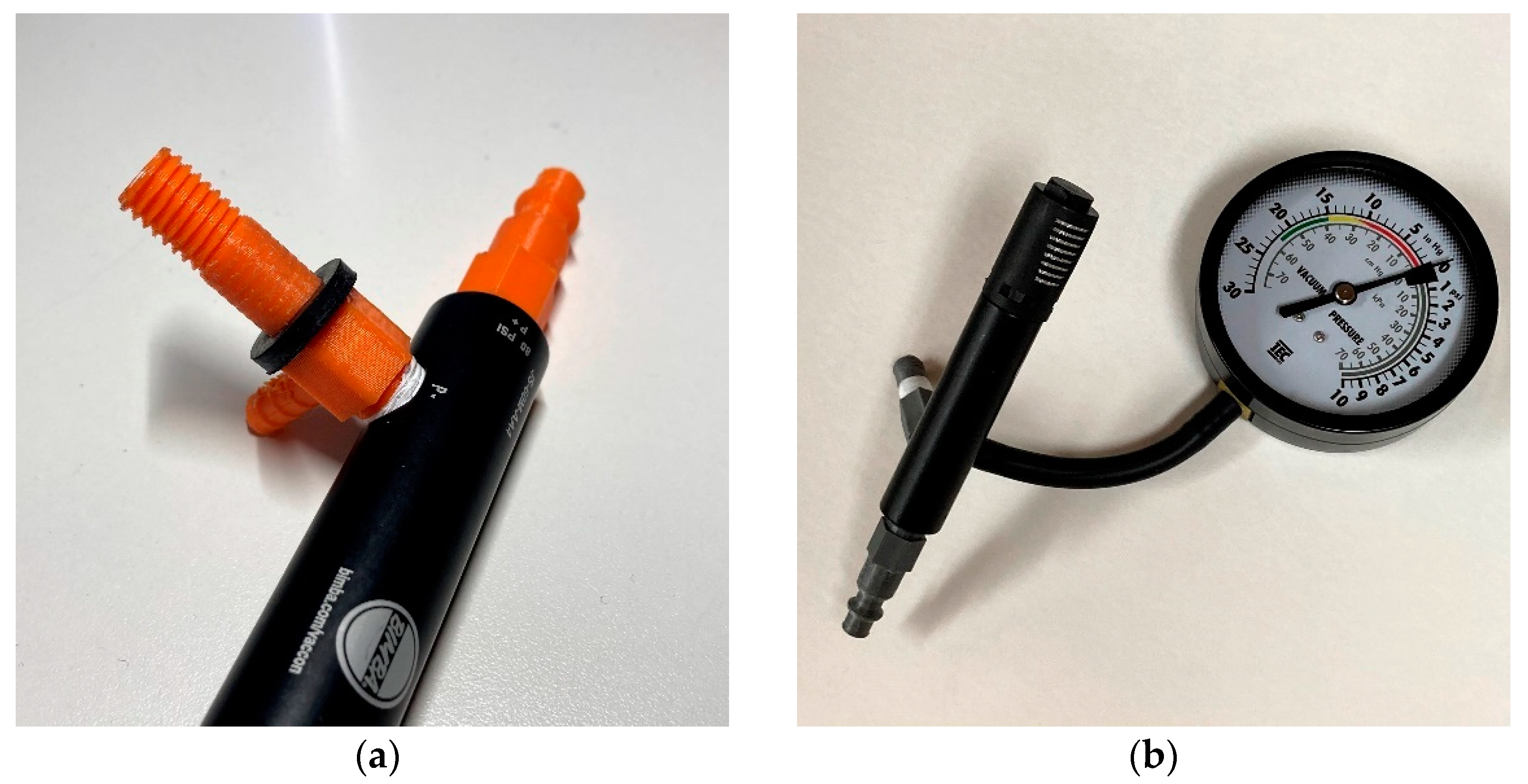
Fixed-Flow Air-Powered Vacuum Pump
$79.75 [37]
Jmmp 05 00052 i002
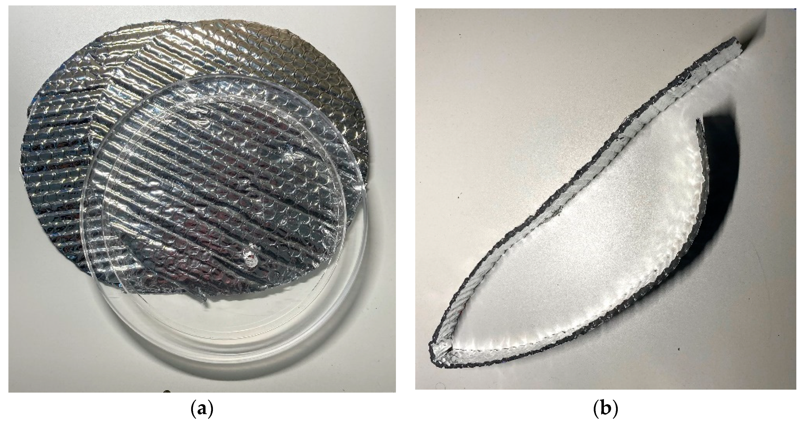
Vacuum Chamber, including:
  • Lid with hole for plumbing
  • M10 Nut
  • M10 Washers (nylon or rubber)
$89.99 [27]
Jmmp 05 00052 i003
10 sq ft Reflectix Double Sided Insulation
$13.57/33.3 sq ft [46]
Jmmp 05 00052 i004
Vacuum Gauge with Rubber Hose
$24.99 [30]
Jmmp 05 00052 i005
1 ft High Temperature Flue Tape
$8.82/15 ft [47]
Jmmp 05 00052 i006
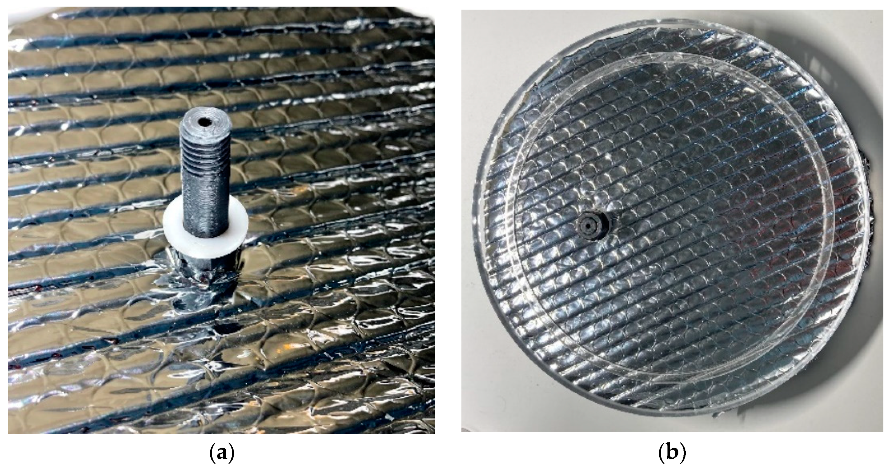
3-D Printed Vacuum Pump Intake Connector [45]
Printed in shown orientation, threads up.
Jmmp 05 00052 i007
3-D Printed Vacuum Pump Vacuum Connector [45]
Printed in shown orientation, fine threads up
Jmmp 05 00052 i008
Thermal Control System
120V Silicone Heating Pad, 1.16 W/cm2
(7.5 W/in2)
19.99 [48]
Jmmp 05 00052 i009
Solid State Relay (5 V Input, 120 VAC/2 A+ output) $25.44 [49] Jmmp 05 00052 i010
1x NTC Thermistor
13.99/5 ea [50]
Jmmp 05 00052 i011
3x 10 kOhm Resistor (or 1x 30 kOhm resistor)
$6.42/100 ea [51]
Jmmp 05 00052 i012
Arduino Microcontroller (Nano)
$20.70 [52]
or derivative
$15.99/3 ea [53]
Jmmp 05 00052 i013
USB-A to USB-mini-B (or USB-micro, or USB-B, depending on the Arduino)
$3.84 [54]
Jmmp 05 00052 i014
1x Solder Breadboard, 3 × 7 cm
$11.21/40 ea [55]
Jmmp 05 00052 i015
Male and Female Header pins:
  • 1 × 2 × 1 M
  • 2 × 15 × 1 F
$5.99/1200 ea [56]
Jmmp 05 00052 i016
22 AWG Hookup Wires:
  • 1 × 160 mm Yellow
  • 1 × 160 mm Black
  • 2 × 20 mm Red
  • 1 × 20 mm Yellow
  • 1 × 20 mm Black
14.95/42 m [57]
Jmmp 05 00052 i017

Appendix C. Wiring Instructions

The pads on the breadboard are labeled on a grid system, rows 1–10 and columns A–X. This grid system is used to indicate locations of connections. In the case of hookup wires, each end of the wire connects to two pads—the pad where the wire is secured, then the pin that the wire is actually connected to. Each end of the wire is labeled in this manner: ‘pad to insert into: pad to solder to’. An example is shown in Figure A1.
Figure A1. Illustration of wire solder labels. The top row is row 10, and it contained a row of header pins. A wire needed to connect to the header pin at L10. To do this, the wire was soldered into L9, then bent over onto L10 (which was already occupied by a header pin) and soldered in place. This wire would be labeled ‘L9:L10′.
Jmmp 05 00052 g0a1
First, the 15 × 1 female header pins were installed on row 10, columns A–O and row 4, columns A–O. These mount the Arduino Nano, with the USB port on the ‘A’ side. Next, the 2 × 1 header pins were installed in row 1, L-M. These headers receive the thermistor’s pre-installed connector.
Next, the reference resistor was soldered into pads B1 and K1:L1. Since three 10 kOhm resistors were in use, they were installed to span that gap, shorted together along the way. This created the voltage divider, with the measurement node at K1:L1.
Two 20 mm red wires were used to connect power to the reference resistor at the top of the voltage divider. The first wire was connected to B3:B4 and B2:B1. The second was connected to C3:C4 and C2:B1. This provided 3.3 V, which is cleaner (less noisy) than 5 V on an Arduino, to the voltage divider and the ADC reference pin on the Arduino [69]. One 20 mm yellow wire was connected to K3:K4 and K2:K1, connecting the measurement node to A7 on the Arduino. To ground the divider, a 20 mm black wire was connected to N3:N4 and M2:M1.
Finally, a 160 mm black wire was connected to N5:N4 with the other end open. Similarly, a 160 mm yellow wire was connected to C9:C10. These wires connect to the input terminals (3 and 4) on the solid-state relay (Figure 10b). The completed circuit is shown in Figure 9.

References

  1. Parikh, D.M. Solids Drying: Basics and Applications. Chem. Eng. 2014, 121, 42–45. [Google Scholar]
  2. Jansen, J. Plastics Engineering—January 2015—Plastic Failure Through Molecular Degradation. Plast. Eng. Jan. 2015, 71, 34–39. [Google Scholar] [CrossRef]
  3. Bozzelli, J. Injection Molding: You Must Dry Hygroscopic Resins. Plastics Technology. 2010. Available online: https://www.ptonline.com/articles/you-must-dry-hygroscopic-resins (accessed on 19 May 2021).
  4. Calovini, L. Everything You Need to Know About Desiccant Drying. Shini USA. 2016. Available online: https://www.shiniusa.com/2016/07/26/everything-you-need-to-know-about-desiccant-drying/ (accessed on 19 May 2021).
  5. Stoughton, P. How to Dry PET for Container Applications. Plastics Technology. 2014. Available online: https://www.ptonline.com/articles/how-to-dry-pet-for-container-applications (accessed on 19 May 2021).
  6. Månsson, A. How Moist Filaments Will Screw up Your 3D-Printing. 3DPrinterChat. 2016. Available online: https://3dprinterchat.com/how-moist-filaments-will-screw-up-your-3d-printing/ (accessed on 19 May 2021).
  7. Dertinger, S.C.; Gallup, N.; Tanikella, N.G.; Grasso, M.; Vahid, S.; Foot, P.J.; Pearce, J.M. Technical pathways for distributed recycling of polymer composites for distributed manufacturing: Windshield wiper blades. Resour. Conserv. Recycl. 2020, 157. [Google Scholar] [CrossRef]
  8. Sanchez, F.A.; Boudaoud, H.; Camargo, M.; Pearce, J.M. Plastic recycling in additive manufacturing: A systematic literature review and opportunities for the circular economy. J. Clean. Prod. 2020, 264. [Google Scholar] [CrossRef]
  9. Little, H.A.; Tanikella, N.G.; Reich, M.J.; Fiedler, M.J.; Snabes, S.L.; Pearce, J.M. Towards Distributed Recycling with Additive Manufacturing of PET Flake Feedstocks. Materials 2020, 13, 4273. [Google Scholar] [CrossRef] [PubMed]
  10. Li, P.; Ramaswamy, S.; Bjegovic, P. Pre-Emptive Control of Moisture Content in Paper Manufacturing Using Surrogate Measurements. Trans. Inst. Meas. Control Trans Inst Meas. Control 2003, 25, 36–56. [Google Scholar] [CrossRef]
  11. Amos, W.A. Report on Biomass Drying Technology; National Renewable Energy Lab.: Golden, CO, USA, 1999. [CrossRef] [Green Version]
  12. Resin Expert. How to Stabilize Wood—Stabilise Wood the Right Way. Available online: https://resin-expert.com/en/guide/how-to-stabilize-wood (accessed on 27 March 2021).
  13. Boundless. 6.14E: Desiccation. In Microbiology; LibreTexts: Davis, CA, USA, 2021. [Google Scholar]
  14. Vega-Mercado, H.; Marcela Góngora-Nieto, M.; Barbosa-Cánovas, G.V. Advances in Dehydration of Foods. J. Food Eng. 2001, 49, 271–289. [Google Scholar] [CrossRef]
  15. Alibert; Ama-fessional Molder. 3D Print Board Filament Dryer Discussion page 1. Available online: https://3dprintboard.com/showthread.php?27550-Filament-Dryer (accessed on 9 June 2020).
  16. Sherman, L.M. Resin Dryers: Which Type Is Right for You? Plastics Technology. 2005. Available online: https://www.ptonline.com/articles/resin-dryers-which-type-is-right-for-you (accessed on 19 May 2021).
  17. Barley, J. Basic Principles of Freeze Drying. Available online: https://www.spscientific.com/freeze-drying-lyophilization-basics/ (accessed on 27 March 2021).
  18. Yao, C.; Qian, X.-D.; Zhou, G.-F.; Zhang, S.-W.; Li, L.-Q.; Guo, Q.-S. A Comprehensive Analysis and Comparison between Vacuum and Electric Oven Drying Methods on Chinese Saffron (Crocus sativus L.). Food Sci. Biotechnol. 2018, 28, 355–364. [Google Scholar] [CrossRef]
  19. 3DXTech. Drying Instructions. Available online: https://www.3dxtech.com/drying-instructions/ (accessed on 8 June 2020).
  20. eSun. EBOX. Available online: http://www.esunchina.net/products/246.html (accessed on 8 June 2020).
  21. 3D Print Board. Filament Dryer. Available online: https://3devo.com/blog/best-ways-to-store-your-3d-printing-filament/ (accessed on 9 June 2020).
  22. CNC Kitchen. Investigating Different Methods of Filament Drying (Dehydrator, Vacuum, Oven & Desiccant). Available online: https://www.cnckitchen.com/blog/cyo43tzz88uqge65xgwz0wv8yvv3rs (accessed on 30 March 2020).
  23. HarvestRight. Home Freeze Dryer. Available online: https://harvestright.com/product/home-freeze-dryer/ (accessed on 30 March 2021).
  24. AMTechniques. Vacuum Filament Dryer. Available online: https://www.kickstarter.com/projects/gertjan-mulder/vacuum-filament-dryer (accessed on 30 March 2021).
  25. Novatec. Vacuum Dryers. Available online: https://www.ptonline.com/knowledgecenter/plastics-drying/dryer-types/vacuum-dryers (accessed on 8 June 2020).
  26. Hubbard, B.R.; Pearce, J.M. Open-Source Digitally Replicable Lab-Grade Scales. Instruments 2020, 4, 18. [Google Scholar] [CrossRef]
  27. SUNCOO 2 Gallon Stainless Steel Vacuum Chamber for Degassing Urethanes, Resins, Silicones and Epoxies. Available online: https://www.amazon.com/SUNCOO-Stainless-Degassing-Urethanes-Silicones/dp/B078K9Q3F9 (accessed on 29 March 2021).
  28. Yunus, A.C.; Michael, A.B. Table A-4 Saturated Water. In Thermodynamics: An Engineering Approach 8e; McGraw Hill Education: New York, NY, USA, 2016; pp. 904–905. ISBN 978-93-392-2165-2. [Google Scholar]
  29. Engineering Toolbox. Water-Boiling Points at Vacuum Pressure. Available online: https://www.engineeringtoolbox.com/water-evacuation-pressure-temperature-d_1686.html (accessed on 29 March 2021).
  30. INNOVA 3620 Vacuum/Carburetor Fuel Pressure Tester. Available online: https://www.amazon.com/INNOVA-3620-Vacuum-Carburetor-Pressure/dp/B000EW0KPY (accessed on 30 March 2021).
  31. CRAFTSMAN 6-Gallon Single Stage Portable Electric Pancake Air Compressor. Available online: https://www.lowes.com/pd/CRAFTSMAN-6-Gallon-Single-Stage-Portable-Electric-Pancake-Air-Compressor/1000595167 (accessed on 30 March 2021).
  32. Blatchley, C.G. Selection of Air Ejectors. Schutte & Koerting. Available online: https://www.s-k.com/technical-references/air_ejector_selection.pdf (accessed on 19 May 2021).
  33. Dandachi, J.M.A. Steam Air Ejector Performance and Its Dimensional Parameters. Ph.D. Thesis, Loughborough University, Loughborough, UK, 1990. Available online: https://hdl.handle.net/2134/7041 (accessed on 19 May 2021).
  34. Hill, G.F.; Sachse, G.W. Venturi Air-Jet Vacuum Ejectors for High-Volume Atmospheric Sampling on Aircraft Platforms; NASA: Washington, DC, USA, 1992; p. 45.
  35. Hall, N. Nozzle Design—Converging/Diverging (CD) Nozzle. Available online: https://www.grc.nasa.gov/WWW/K-12/airplane/nozzled.html (accessed on 18 August 2020).
  36. Hydraulics Pneumatics. Compressed Air Guide: Pull, Don’t Push. Hydraulics & Pneumatics. 2014. Available online: https://www.hydraulicspneumatics.com/technologies/air-compressors/article/21884511/compressed-air-guide-pull-dont-push (accessed on 19 May 2021).
  37. Fixed-Flow Air-Powered Vacuum Pump. Available online: https://www.mcmaster.com/9997K15/ (accessed on 29 March 2021).
  38. BAPI. Thermistor vs RTD Temperature Measurement Accuracy—Application Note. Available online: https://www.bapihvac.com/application_note/thermistor-vs-rtd-temperature-measurement-accuracy-application-note/ (accessed on 9 June 2020).
  39. Williams, A. Thermistors and 3D Printing. Hackaday. 2017. Available online: https://hackaday.com/2017/12/15/thermistors-and-3d-printing/ (accessed on 19 May 2021).
  40. Banzi, M.; Shiloh, M. Getting started with Arduino: The Open Source Electronics Prototyping Platform; Maker Media, Inc.: Sebastopol, CA, USA, 2014. [Google Scholar]
  41. Microstar Laboratories. Calibrate Thermistors. Available online: http://www.mstarlabs.com/sensors/thermistor-calibration.html (accessed on 29 March 2021).
  42. Amtherm. The Secret to Successful Thermistor Beta Calculations. Available online: https://www.ametherm.com/blog/thermistors/thermistor-beta-calculations (accessed on 7 July 2020).
  43. Electronics Tutorials. Thermistors and NTC Thermistors. Available online: https://www.electronics-tutorials.ws/io/thermistors.html (accessed on 22 March 2021).
  44. Tempco. Duraband Maximum Watt Densities. Available online: https://www.tempco.com/Tempco/Resources/01-Band-Resources/DurabandsWattDnsty.pdf (accessed on 30 March 2020).
  45. Hubbard, B.; Pearce, J.M. Open Source Vacuum Oven for Low-Temperature Drying. Available online: https://osf.io/vf2b8/ (accessed on 19 May 2021).
  46. Reflectix 16 in. x 25 Ft. Double Reflective Insulation Roll with Staple Tab Edge-ST16025. Available online: https://www.homedepot.com/p/Reflectix-16-in-x-25-ft-Double-Reflective-Insulation-Roll-with-Staple-Tab-Edge-ST16025/100012574 (accessed on 30 March 2021).
  47. 3M High Temperature Flue Tape, High Heat Sealing Tape up to 600 Degrees, 15-Foot Roll. Available online: https://www.amazon.com/3M-High-Temperature-Flue-15-Foot/dp/B00004Z4DS (accessed on 30 March 2021).
  48. ABN Silicone Heating Pad 120V—4 × 5 Inch Universal Engine Heater Car Oil Pan Heater Pad, 150W Electric Heater Pad. Available online: https://www.amazon.com/ABN-Automotive-Electric-Silicone-Heating/dp/B077J5DSFJ (accessed on 30 March 2021).
  49. G3NA-210B-UTU DC5-24 Omron Automation and Safety. Available online: https://www.mouser.com/ProductDetail/653-G3NA210BUTUDC524 (accessed on 30 March 2021).
  50. Creality 3D Printer NTC Thermistor Temp Sensor 100K for Ender 3/Ender 3 Pro/Ender 5/CR-10/CR-10S. Available online: https://www.amazon.com/Printer-Thermistor-Sensor-Reprap-Comgrow/dp/B0714MR5BC (accessed on 30 March 2021).
  51. E-Projects 100EP51210K0 10k Ohm Resistors, 1/2 W, 5% (Pack of 100). Available online: https://www.amazon.com/Projects-100EP51210K0-10k-Resistors-Pack/dp/B0185FIOTA (accessed on 30 March 2021).
  52. Arduino Nano. Available online: https://store.arduino.cc/usa/arduino-nano (accessed on 30 March 2021).
  53. ELEGOO Nano Board CH340/ATmega328P Without USB Cable, Compatible with Arduino Nano V3.0 (Nano x 3 Without Cable). Available online: https://www.amazon.com/ELEGOO-Arduino-ATmega328P-Without-Compatible/dp/B0713XK923 (accessed on 30 March 2021).
  54. Monoprice 3-Feet USB A to Mini-B 5pin 28/28AWG Cable (103896) Black. Available online: https://www.amazon.com/Monoprice-3-Feet-mini-B-28AWG-103896/dp/B003L18SHC/ (accessed on 30 March 2021).
  55. Geekcreit 40pcs FR-4 2.54mm Double Side Prototype PCB Printed Circuit Board. Available online: https://www.banggood.com/Geekcreit-40pcs-FR-4-2_54mm-Double-Side-Prototype-PCB-Printed-Circuit-Board-p-995732.html (accessed on 30 March 2021).
  56. DEPEPE 30 Pcs 40 Pin 2.54mm Male and Female Pin Headers for Arduino Prototype Shield. Available online: https://www.amazon.com/DEPEPE-2-54mm-Headers-Arduino-Prototype/dp/B074HVBTZ4/ (accessed on 30 March 2021).
  57. Plusivo 22AWG Hook up Wire Kit—600V Tinned Stranded Silicone Wire of 6 Different Colors x 23 Ft Each. Available online: https://www.plusivo.com/home/67-plusivo-22awg-hook-up-wire-kit-600v-tinned-stranded-silicone-wire-of-6-different-colors-x-23-ft-each.html (accessed on 30 March 2021).
  58. Reflectix Inc. Installation Instructions for Reflectix, Inc. Double Reflective Insulation. Available online: https://images.homedepot-static.com/catalog/pdfImages/5a/5ab3af4c-631f-416d-af7c-b7aeb41f51a2.pdf (accessed on 30 March 2021).
  59. FreeCAD. Available online: https://www.freecadweb.org/ (accessed on 30 March 2021).
  60. OpenSCAD. Available online: http://openscad.org (accessed on 30 March 2021).
  61. Kirshner, D. Thread-Drawing Modules for OpenSCAD. Available online: https://dkprojects.net/openscad-threads/ (accessed on 30 March 2021).
  62. GNU General Public License Version 3. Available online: https://www.gnu.org/licenses/gpl-3.0.en.html (accessed on 30 March 2021).
  63. Corona688. OpenSCAD NPT/Tsmthread 0.4. Available online: https://www.thingiverse.com/thing:3391213 (accessed on 30 March 2021).
  64. Creative Commons—Attribution-NonCommercial 3.0 Unported—CC BY-NC 3.0. Available online: https://creativecommons.org/licenses/by-nc/3.0/ (accessed on 30 March 2021).
  65. Anzalone, G.; Wijnen, B.; Pearce, J. Multi-Material Additive and Subtractive Prosumer Digital Fabrication with a Free and Open-Source Convertible Delta RepRap 3-D Printer. Rapid Prototyp. J. 2015, 21, 506–519. [Google Scholar] [CrossRef] [Green Version]
  66. Ultimaker. Ultimaker Cura 4.7.1. Available online: https://github.com/Ultimaker/Cura (accessed on 30 March 2021).
  67. Buckeye Hydro. Should I Use Teflon Tape? Available online: https://www.buckeyehydro.com/blog/should-i-use-teflon-tape/ (accessed on 19 May 2021).
  68. SciPy Optimization and Root Finding (Scipy.Optimize). Available online: https://docs.scipy.org/doc/scipy/reference/optimize.html (accessed on 30 March 2021).
  69. Hrisko, J. Arduino Thermistor Theory, Calibration, and Experiment. Maker Portal. 2019. Available online: https://makersportal.com/blog/2019/1/15/arduino-thermistor-theory-calibration-and-experiment (accessed on 19 May 2021).
  70. Salimov, Y. NTC_Thermistor. Available online: https://github.com/YuriiSalimov/NTC_Thermistor (accessed on 30 March 2021).
  71. Novatec. Hygroscopic VS Non-Hygroscopic Resins. Available online: https://www.ptonline.com/knowledgecenter/plastics-drying/resin-types/hygroscopic-vs-non-hygroscopic-resins (accessed on 8 June 2020).
  72. Lee, J.H.; Lim, K.; Hahm, W.; Kim, S. Properties of Recycled and Virgin Poly(Ethylene Terephthalate) Blend Fibers. J. Appl. Polym. Sci. 2013, 128. [Google Scholar] [CrossRef]
  73. Zander, N.; Gillan, M.; Burckhard, Z.; Gardea, F. Recycled Polypropylene Blends as Novel 3D Printing Materials. Addit. Manuf. 2018, 25. [Google Scholar] [CrossRef]
  74. Idrees, M.; Jeelani, S.; Rangari, V. 3D Printed Sustainable Biochar-Recycled PET Composite. Acs Sustain. Chem. Eng. 2018, 6. [Google Scholar] [CrossRef]
  75. Baechler, C.; DeVuono, M.; Pearce, J.M. Distributed recycling of waste polymer into RepRap feedstock. Rapid Prototyp. J. 2013, 19, 118–125. [Google Scholar] [CrossRef]
  76. Woern, A.L.; McCaslin, J.R.; Pringle, A.M.; Pearce, J.M. RepRapable Recyclebot: Open source 3-D printable extruder for converting plastic to 3-D printing filament. HardwareX 2018, 4, e00026. [Google Scholar] [CrossRef]
  77. Karegoudar, T.B.; Pujar, B.G. Degradation of Terephthalic Acid by a Bacillus Species. FEMS Microbiol. Lett. 1985, 30, 217–220. [Google Scholar] [CrossRef]
  78. Vamsee-Krishna, C.; Mohan, Y.; Phale, P. Biodegradation of Phthalate Isomers by Pseudomonas Aeruginosa PP4, Pseudomonas Sp. PPD and Acinetobacter Lwoffii ISP4. Appl. Microbiol. Biotechnol. 2006, 72, 1263–1269. [Google Scholar] [CrossRef]
  79. Ritala, A.; Häkkinen, S.T.; Toivari, M.; Wiebe, M.G. Single Cell Protein—State-of-the-Art, Industrial Landscape and Patents 2001–2016. Front. Microbiol. 2017, 8, 2009. [Google Scholar] [CrossRef]
  80. García Martínez, J.B.; Egbejimba, J.; Throup, J.; Matassa, S.; Pearce, J.; Denkenberger, D. Potential of Microbial Protein from Hydrogen for Preventing Mass Starvation in Catastrophic Scenarios. Sustain. Prod. Consum. 2020, 25, 234–247. [Google Scholar] [CrossRef]
  81. García Martínez, J.B.; Pearce, J.M.; Cates, J.; Denkenberger, D. Methane Single Cell Protein: Securing Protein Supply During Global Food Catastrophes. Available online: https://osf.io/94mkg (accessed on 19 May 2021).
  82. Rosewill. Countertop Portable Electric Food Fruit Dehydrator Machine with Adjustable Thermostat, BPA-Free, 5-Tray, RHFD-15001. Available online: /ip/Rosewill-Countertop-Portable-Electric-Food-Fruit-Dehydrator-Machine-with-Adjustable-Thermostat-BPA-Free-5-Tray-RHFD-15001/51409615 (accessed on 31 March 2021).
  83. P3. Kill A Watt Meter—Electricity Usage Monitor. Available online: http://www.p3international.com/products/p4400.html (accessed on 31 March 2021).
  84. MH Build Series PLA Filament—1.75mm (1 kg). Available online: https://www.matterhackers.com/store/3d-printer-filament/175mm-pla-filament-red-1-kg (accessed on 31 March 2021).
  85. Pearce, J.M. Economic Savings for Scientific Free and Open Source Technology: A Review. HardwareX 2020, 8, e00139. [Google Scholar] [CrossRef]
  86. YamatoADP. Series 220V Vacuum Drying Ovens—Ovens and Furnaces, Vacuum Ovens. Available online: https://www.fishersci.com/shop/products/yamato-adp-series-220v-vacuum-drying-ovens-2/1326320 (accessed on 31 March 2021).
  87. Oberloier, S.; Pearce, J. General Design Procedure for Free and Open-Source Hardware for Scientific Equipment. Designs 2017, 2, 2. [Google Scholar] [CrossRef] [Green Version]
  88. Gibb, A. Building Open Source Hardware: DIY Manufacturing for Hackers and Makers; Pearson Education: London, UK, 2014. [Google Scholar]
  89. Chagas, A.M. Haves and Have Nots Must Find a Better Way: The Case for Open Scientific Hardware. PLoS Biol. 2018, 16, e3000014. [Google Scholar] [CrossRef] [Green Version]
  90. Powell, A. Democratizing Production through Open Source Knowledge: From Open Software to Open Hardware. Media Cult. Soc. 2012, 34, 691–708. [Google Scholar] [CrossRef] [Green Version]
  91. Vacuum Science World. The Fundamentals of Vacuum Science. Available online: https://www.vacuumscienceworld.com/vacuum-science (accessed on 29 March 2021).
  92. ABLAZE 3 Gallon Stainless Steel Vacuum Degassing Chamber and 3 CFM Single Stage Pump Kit. Available online: https://www.amazon.com/ABLAZE-Gallon-Stainless-Degassing-Chamber/dp/B076KNYCZ6/ (accessed on 29 March 2021).
  93. VAC AERO. International Gas Ballasting of Mechanical Oil Sealed Rotary Vacuum Pumps. Available online: https://vacaero.com/information-resources/vacuum-pump-technology-education-and-training/666-gas-ballasting-of-mechanical-oil-sealed-rotary-vacuum-pumps.html (accessed on 30 July 2020).
  94. Schach, A. How to Select the Right Vacuum Pump; Labconco: Kansas City, MO, USA, 2016. [Google Scholar]
Figure 1. Insulation was cut to fit the specific vacuum chamber that was purchased. (a) Circles of insulation to cover the base and lid; (b) a strip of insulation to be wrapped around the circumference of the chamber to build an air gap.
Jmmp 05 00052 g001
Figure 2. Air ejector connector cross-sections, highlighting internal geometry where air flows. (a) Intake connector, where high pressure air enters the ejector; (b) vacuum connector, where evacuated air flows from the chamber to the ejector and vacuum pressure is measured.
Jmmp 05 00052 g002
Figure 3. Assemble the air ejector. (a) Thread the 3-D printed connectors into the air ejector, using PTFE tape if necessary; (b) attach the vacuum gauge to the hose barb. Note that the same parts were printed in orange (left) and grey (right) PLA.
Jmmp 05 00052 g003
Figure 4. The air ejector is driven by compressed air, which creates a vacuum pressure inside the ejector, pulling air through the vacuum connector into the stream of compressed air. The exhaust is delivered into the atmosphere through a diffuser that reduces airflow noise.
Jmmp 05 00052 g004
Figure 5. Process to connect the air ejector to the lid. Note that the photographed part is grey here, where it was orange in prior photos. (a) Feeding the vacuum connector through the insulation, then an M10 washer (nylon or rubber); (b) feeding the vacuum connector through the lid, then another washer, then secure with an M10 nut.
Jmmp 05 00052 g005
Figure 6. If installed, the heater power cable and sensor wires may be fed up the wall of the chamber for strain relief, but this is not required.
Jmmp 05 00052 g006
Figure 7. Install insulation on the chamber wall. (a) First, attach strips of insulation to build an air gap and span the protruding components on the chamber walls; (b) Next, install the large piece of insulation, fully covering the walls of the chamber.
Jmmp 05 00052 g007
Figure 8. The circuit is a voltage divider and a pair of signal wires to control the relay.
Jmmp 05 00052 g008
Figure 9. The completed circuit is wired to connect to a relay and measure a single thermistor.
Jmmp 05 00052 g009
Figure 10. Assembly of the electronics for the thermal controller. (a) The Arduino installed on the circuit; (b) the signal wires attached to the relay.
Jmmp 05 00052 g010
Figure 11. The heating element was adhered to the base of the chamber, with the thermistor secured on the interface.
Jmmp 05 00052 g011
Figure 12. The power cable was prepared for connection to the relay. (a) First, it was cut in half. Only one wire needed to be cut, but both were cut in this case. (b) Next, one pair of wires was immediately re-joined with a wire nut.
Jmmp 05 00052 g012
Figure 13. The power cable was secured into the load terminals of the relay.
Jmmp 05 00052 g013
Figure 14. The fully assembled vacuum oven.
Jmmp 05 00052 g014
Figure 15. The test setup for measuring temperature gradient. (a) Three thermistors were mounted on a 3-D printed jig, mounting them 0, 25, and 50 mm above the base of the chamber. (b) For the second test, a heat sink was added in the mix of rPET to aid heat transfer throughout the material.
Jmmp 05 00052 g015
Figure 16. The full Steinhart–Hart Equation yields this temperature curve, showing the thermistor’s sensitivity decreasing as the temperature increases.
Jmmp 05 00052 g016
Figure 17. The calculated Beta values have varying accuracy as a function of resistance. These curves show that Beta of 3920 or 3950 maintain an error within 1 °C for the majority of the temperature range under assessment.
Jmmp 05 00052 g017
Figure 18. Temperature gradient measurements. (a) Chamber loosely packed with rPET; (b) chamber loosely packed with rPET, plus a metal cylinder, referred to as a heat sink.
Jmmp 05 00052 g018
Figure 19. Temperature gradient measurements with the inside surface temperature used for control. (a) Chamber empty and open to the air, average heater temperature 79 °C at steady state. Note that the 25 and 50 mm curves lie on top of each other, since both are measuring air temperature inside the chamber; (b) chamber loosely packed with rPET, average heater temperature 68 °C at steady state.
Jmmp 05 00052 g019
Figure 20. Dehydration measurements on small (10 g) samples of rPET. Increasing the oven temperature from 70 (left) to 80 °C (right) caused a 40% decrease in drying time. (a) Sample percent initial mass with the vacuum oven set to 70 °C. The vacuum oven was 25% slower than the dehydrator at this setting; (b) Sample percent initial mass with the vacuum oven set to 80 °C. In this case, the vacuum oven was 40% faster than the dehydrator. (c) The energy consumed during the 70 °C test. The dashed lines are summed in the blue aggregate energy for the oven. (d) The energy consumed during the 80 °C test.
Jmmp 05 00052 g020
Figure 21. Dehydration of large (350g) samples of rPET. This test was cut short because it clearly indicated that the vacuum oven could not manage the large mass of plastic and water. (a) The percentage of initial mass as a function of time. (b) The energy consumption of each device. The energy consumption of the vacuum is shown as an aggregate of the two components, the heater and the vacuum.
Jmmp 05 00052 g021
Figure 22. 500 mg samples of the consortium were dehydrated in a petri dish. (a) The wet culture, prior to drying; (b) the fully dehydrated culture.
Jmmp 05 00052 g022
Figure 23. Dehydration measurements on consortium of microorganisms. (a) Percent initial mass for each sample; (b) energy consumption. The dashed oven vacuum and oven heater curves were summed to form the aggregate oven curve.
Jmmp 05 00052 g023
Figure 24. The dried filament showed significantly stronger layer adhesion and smoother surface finish.
Jmmp 05 00052 g024
Figure 25. A 1 kg spool of PLA filament was dried in the vacuum oven. The change in mass was around 0.4 g, compared to the initial mass of 1245.7 g.
Jmmp 05 00052 g025
Table 1. Print Settings for PLA.
PropertyValue
Layer Height0.2 mm
Wall Thickness2 mm
Top/Bottom Thickness0.8 mm
InfillCubic, 20%
Nozzle Temperature210 °C
Print SpeedInfill/Support: 70 mm/s, Wall: 35 mm/s
Outer Wall Speed35 mm/s
RetractionYes
Print CoolingNo
SupportBuild-plate only, 50 deg, 15% density
Adhesion TypeBrim
Table 2. Optimized reference resistances for several operating temperature ranges.
Temperature Range (°C)Reference Resistance, R0 (kOhm)ADC Range Utilized
50–60309%
60–70219%
70–80158%
50–802125%
Table 3. Thermistor calibration measurements.
Temperature (°C)Reference Resistance, R0 (kOhm)
25100
0310
1007.1
Table 4. Steinhart–Hart full model calibration.
CoefficientValue
Ka6.9 × 10−4
Kb2.1 × 10−4
Kc1.3 × 10−7
Table 5. Steinhart–Hart simplified model calibration.
Temperatures UsedBeta
25, 03690
0, 1003850
25, 1003920
Nominal3950
Table 6. Summary of the test results.
Test DescriptionDeviceDrying TimeEnergy Consumed (Average Specific Energy)
10 g rPET, 70 °CVacuum Oven75 min0.51 kWh (1.55 kWh/g)
Dehydrator60 min0.23 kWh (0.70 kWh/g)
10 g rPET, 80 °CVacuum Oven45 min0.28 kWh (0.80 kWh/g)
Dehydrator75 min0.30 kWh (0.83 kWh/g)
350 g rPETVacuum Oven180+ min1.30+ kWh (0.12 kWh/g)
Dehydrator60 min0.45 kWh (0.04 kWh/g)
BiomassVacuum Oven75 min0.55 kWh (1.17 kWh/g)
Dehydrator150 min0.56 kWh (1.30 kWh/g)
Table 7. Cost breakdown of the vacuum oven.
ComponentUp-Front Cost as Purchased (USD)Effective Cost (USD)
Heater$116.60$58.17
Vacuum$316.12$298.39
Total$432.72$356.56
Table 8. Cost comparison of the open source vacuum oven with other devices on the market.
Type of DryerCostPercent Savings
Vacuum Oven [86]$2920.0087.8%
Vacuum Filament Drier [24]$2295.0084.5%
Freeze Dryer [23]$2195.0083.8%
Publisher’s Note: MDPI stays neutral with regard to jurisdictional claims in published maps and institutional affiliations.

