Article

Finite-Time Robust Flight Control of Logistic Unmanned Aerial Vehicles Using a Time-Delay Estimation Technique

1
School of Aeronautics, Nanjing University of Aeronautics and Astronautics, Nanjing 210016, China
2
School of Intelligent Manufacturing, Wenzhou Polytechnic, Wenzhou 325000, China
3
Wenzhou Institute, University of Chinese Academy of Sciences, Wenzhou 325000, China
4
School of Mechanical and Electrical Engineering, Wenzhou University, Wenzhou 325000, China
*
Authors to whom correspondence should be addressed.
Drones 2024, 8(2), 58; https://doi.org/10.3390/drones8020058
Submission received: 3 January 2024 / Revised: 26 January 2024 / Accepted: 7 February 2024 / Published: 8 February 2024

Abstract

:
This paper proposes a cascaded dual closed-loop control strategy that incorporates time delay estimation and sliding mode control (SMC) to address the issue of uncertain disturbances in logistic unmanned aerial vehicles (UAVs) caused by ground effects, crosswind disturbances, and payloads. The control strategy comprises a position loop and an attitude loop. The position loop, which functions as the outer loop, employs a proportional–integral–derivative (PID) sliding mode surface to eliminate steady-state error through an integral component. Conversely, the attitude loop, serving as the inner loop, utilizes a fast nonsingular terminal sliding mode approach to achieve finite-time convergence and ensure a quick system response. The time-delay estimation technique is employed for the online estimation and real-time compensation of unknown disturbances, while SMC is used to enhance the robustness of the control system. The combination of time-delay estimation and SMC offers complementary advantages. The stability of the system is proven using Lyapunov theory. Hardware-in-the-loop simulation and flight tests demonstrate that the control law can achieve a smooth and continuous output. The proposed control strategy can be effectively applied in complex scenarios, such as hovering, crash recovery, and high maneuverability flying, with significant practicality in engineering applications.

1. Introduction

The field of rotorcraft logistic unmanned aerial vehicles (UAVs) [1] is rapidly advancing, transforming from a concept into a practical and productive force [2]. During operation, rotorcraft logistic UAVs require the ability to hover, maneuver in flight, and possess strong fault tolerance and self-rescue capabilities [3]. These rotorcraft UAVs exhibit complex physical characteristics, including nonlinearity, under-actuation, and strong coupling [4]. The unique nature of logistic operations imposes specific requirements on rotorcraft UAVs [5]. For instance, during ultralow altitude cargo delivery, precise hovering or slow landing is essential. At altitudes less than 2–3 times the size of the UAV, the ground effect becomes noticeable [6], leading to downwash airflow and lateral crosswinds caused by the Bernoulli effect, which impact flight stability. Furthermore, rotorcraft logistic UAVs need to achieve high-speed and high-maneuverability flight while carrying a payload [7]. Due to their low-altitude operation, rotorcraft UAVs must possess fault tolerance and self-rescue capabilities [8] to prevent accidents caused by external interference [9]. Ensuring robust control of rotorcraft logistic UAVs under the combined effects of ground effects, crosswind disturbances, payloads, and failures is a significant challenge [10]. At the current stage of research, the focus is predominantly on designing robust controllers for achieving the precise control of UAV attitude under multiple disturbance effects [11]. Commonly employed control algorithms include both linear and nonlinear control algorithms [12,13]. The proportional–integral–derivative (PID) control algorithm [14], a traditional linear control algorithm, is widely utilized in UAVs, such as in the renowned open-source flight control system Pixhawk 4 [15]. However, PID control, as a linear controller, is unable to adapt to the nonlinearity and variety of complex operating conditions of rotorcraft logistic UAVs [16]. In contrast, nonlinear control methods such as sliding mode control (SMC) [17], fuzzy control [18], optimal control [19], and neural network control [20] exhibit enhanced robustness. Fuzzy control necessitates prior knowledge of the controlled object to establish a fuzzy rule base [21], while optimal control and neural network control entail solving complex mathematical optimization problems with intricate processes [22]. On the other hand, SMC [23] successfully eliminates the uncertainties, nonlinearity, and disturbances of the system through the introduction of a sliding mode surface. This approach is resilient to disturbances caused by parameter changes, external interference, and noise, with a prompt response to system dynamics and a higher closed-loop bandwidth [24]. Moreover, the SMC controller boasts a straightforward structure with a low computational burden and easy implementation [25]. In this research, instead of utilizing cascaded PID [26], the SMC controller will be employed to construct a cascaded dual-loop SMC controller.
The cascade inner–outer control methodology [27] is employed to enhance the control stability and response speed in complex multi-input multi-output and underactuated systems [28]. By implementing a hierarchical and decoupled structure, this approach enables robust control. In cascade inner–outer control, the bandwidth of the inner loop is set at 5 to 10 times larger than the bandwidth of the outer loop [29]. The inner loop controller is designed to swiftly respond to and eliminate fast dynamic instabilities of the system [30]. Moreover, the outer loop controller is responsible for controlling the slow dynamics of the system to achieve precise control.
In the context of UAV control, the inner loop corresponds to the attitude loop, which acquires the desired pitch, roll, and yaw moments. Conversely, the outer loop pertains to position control and is utilized to obtain the desired thrust and provide the reference input for the inner loop. Over the years, the SMC theory has made significant advancements. The fast nonsingular terminal sliding mode (FNTSM) [31,32] has emerged as a groundbreaking development that addresses chattering issues and achieves a finite-time convergence of the system state by introducing a nonsingular terminal mode in the state space [33]. To attain a swift response in attitude control, the FNTSM is employed as the inner loop controller. In the outer loop, the traditional PD-type sliding surface is further refined into a PID-type sliding surface, integrating an integral term to eliminate steady-state error and enhance position control accuracy [34]. Due to the intricacies of operating conditions and uncertainties in payloads, establishing an accurate mathematical model for rotorcraft logistic UAVs is a considerable challenge. A disturbance observer (DOB) [35] is a commonly utilized tool in robust control for obtaining the nominal model of a controlled object. However, the performance of a DOB relies on its structural design and parameter tuning, which can be intricate and time-consuming. Furthermore, the effectiveness of the DOB depends on the observability of the system. With the need for a simple controller structure and low computational cost in practical engineering, this paper introduces the time delay estimation (TDE) technique [36] into SMC. The TDE technique estimates the current system dynamics and disturbances based on the previous system dynamics [37]. It has been extensively employed in controlling piezoelectric ceramics, hydraulic cylinders, and servo robots to estimate time-delay signals, friction forces, modeling errors, and noise disturbances. Consequently, this paper incorporates the TDE technique into the control of rotorcraft logistic UAVs to achieve the online estimation and real-time compensation of system states and external disturbances. This enables the robust controller to have a comprehensive multibody dynamics model.
To demonstrate the effectiveness of the proposed algorithm, complex scenarios such as hovering, crash recovery, and high maneuvering flight scenarios are experimentally studied to simulate the actual working conditions of a rotor logistic UAV. The contributions of this paper are as follows:
  • Construction of a cascaded dual-loop SMC controller. The inner loop adopts the fast nonsingular terminal sliding mode to achieve the finite-time convergence of the system state and improve the response speed. The outer loop employs a PID-type sliding mode surface to enhance the control accuracy.
  • TDE technology is introduced for the robust control of rotor logistic UAVs to achieve the online estimation and real-time compensation of unknown disturbances, thereby improving the nominal dynamic model of the controlled object.
  • Flight capability tests of the rotor logistic UAV are conducted in three complex scenarios to verify the ability of the proposed algorithm to hover, maneuver flight, and perform self-recovery during fault tolerance.
The remainder of this paper is organized as follows: Section 2 describes the dynamic modeling, Section 3 discusses the controller design and stability analysis, Section 4 presents the simulation and experiments, and finally, Section 5 concludes the paper.

2. Dynamic Modeling of Quadcopter UAVs

The structure of a rotorcraft logistic UAV with an “X”-shaped layout, as shown in Figure 1, is depicted. In the figure, O b X b Y b Z b represents the body-fixed coordinate system with the origin located at the center of gravity of the UAV, while O e X e Y e Z e represents the earth-based coordinate system. The position vector Ε = [ x , y , z ] T and attitude vector Θ = [ ϕ , θ , ψ ] T are defined in the Earth coordinate system, where θ ,   ϕ ,   ψ denote the pitch angle, roll angle, and yaw angle, respectively [24].
In accordance with Newton’s laws of motion, the position kinematics model of a rotorcraft logistics UAV is formulated [35]:
[ x ¨ y ¨ z ¨ ] = [ F 1 + F 2 + F 3 + F 4 m ( cos ψ sin θ cos ϕ + sin ψ sin ϕ ) k 1 x ˙ m F 1 + F 2 + F 3 + F 4 m ( sin ψ sin θ cos ϕ cos ψ sin ϕ ) k 2 y ˙ m F 1 + F 2 + F 3 + F 4 m cos ϕ cos θ g k 3 z ˙ m ] ,
In this context, Ε ˙ = [ x ˙ , y ˙ , z ˙ ] T represents the velocity vector in the Earth’s coordinate system, Ε ¨ = [ x ¨ , y ¨ , z ¨ ] T denotes the acceleration vector, g signifies the gravitational acceleration, and F 1 , F 2 , F 3 , and F 4 , respectively, denote the thrusts provided by individual motors. k 1 , k 2 , and k 3 represent the coefficients of translational aerodynamic resistance in three directions.
Based on Euler’s laws, an attitude dynamics model of a rotorcraft logistics UAV is formulated.
[ ϕ ¨ θ ¨ ψ ¨ ] = [ ( F 1 F 2 F 3 + F 4 ) l J y y k 4 l J y y ϕ ˙ ( F 1 + F 2 F 3 F 4 ) l J x x k 5 l J x x θ ˙ ( F 1 F 2 + F 3 F 4 ) l J z z k 6 l J z z ψ ˙ ] ,
In this context, J = diag ( J yy , J x x , J zz ) represents the moment of inertia about the body axis, l denotes the distance from the body center to the motor axis, and k 4 , k5, and k 6 , and represent the torque coefficients of rotational aerodynamic resistance in three directions.
Based on the force relationships of the “X”-shaped layout, the control inputs of the rotorcraft logistics UAVs are defined.
U = { u 1 = F 1 + F 2 + F 3 + F 4 u 2 = ( F 1 F 2 F 3 + F 4 ) l J y y u 3 = ( F 1 + F 2 F 3 F 4 ) l J x x u 4 = ( F 1 F 2 + F 3 F 4 ) l J zz ,
In this context, u 1 , u 2 , u 3 and u 4 represent the control inputs for the throttle, roll, pitch, and yaw, respectively. Substituting these values into Equations (1) and (2), we obtain
{ x ¨ = u 1 m ( cos ψ sin θ cos ϕ + sin ψ sin ϕ ) k 1 x ˙ m y ¨ = u 1 m ( sin ψ sin θ cos ϕ cos ψ sin ϕ ) k 2 y ˙ m z ¨ = u 1 m cos ϕ cos θ g k 3 z ˙ m ϕ ¨ = u 2 k 4 l J yy ϕ ˙ θ ¨ = u 3 k 5 l J xx θ ˙ ψ ¨ = u 4 k 6 l J zz ψ ˙ .

3. Controller Design and Stability Analysis

3.1. Position Loop Controller Design

The objective of rotorcraft logistics UAV controller design is to obtain a nonlinear robust controller that can accurately track desired trajectories even in the presence of adverse factors such as ground effects and crosswind disturbances.
Taking the position controller in the direction of gravity as an example, the design process of the position controller is explained. The desired displacement, velocity, and acceleration in the direction of gravity are defined as z d , z ˙ d and z ¨ d , respectively. The position error, velocity error, and acceleration error in the direction of gravity are defined as e z = z d z , e ˙ z = z ˙ d z ˙ , e ¨ z = z ¨ d z ¨ .
The dynamic equation of the direction of gravity in Equation (4) is simplified as
u 1 = m z ¨ + m g + P z .
In the equation, P z = u 1 u 1 cos ϕ cos θ + k 3 z ˙ + δ z , and the term δ z can be regarded as a complex term that encompasses unknown factors such as modeling errors, air resistance, and external disturbances in the direction of gravity for logistics UAVs.
A linear second-order dynamic equation for the position error is expressed as follows:
e ¨ z + K P Z e z + K I Z e ˙ z = 0 .
where K P Z and K I Z are positive parameters to be adjusted.
To accomplish this, a PID-type sliding surface is designed, and the objective is to achieve s z = 0 . The sliding surface is defined as follows:
s z = e ˙ z + K P Z e z + K I Z e z d τ .
The technique of the fast-approaching law is employed [38]:
s ˙ z = s z + β z sig ( s z ) ρ z .
where β z > 0 and 0 < ρ z < 1 , and the operator “ sig ( ) a = | | a sign ( ) ” is defined for the purpose of simplifying the expression.
The design of an SMC controller with a fast-approaching law and a PID-type sliding surface is presented below:
u 1 = u b + u c .
where u b = m ( u a + β z sig ( s ) ρ z + g ) , u c = P ^ z , and u a = z ¨ d + K P z e ˙ z + K I z e z .
To achieve the accurate estimation of parameter P z in Equation (5) and simplify the controller structure, the TDE technique is employed to obtain an estimated value P ^ z for parameter P z . The expression for P ^ z is given as follows:
P ^ z ( t ) P z ( t L ) = u 1 ( t L ) m z ¨ ( t L ) m g .
In the equation, t represents the current time, L represents the time delay, which is typically kept consistent with the time step of the control system, P z ( t ) and P z denote the same variable, and P ^ z ( t ) and P ^ z represent the same variable.
By substituting Equation (10) into Equation (9), the control law based on the TDE technique can be expressed as follows:
u 1 = m ( z ¨ d + K P Z e ˙ z + K I Z e z + β Z s i g ( s ) ρ Z + g ) FPIDSMC + u 1 ( t L ) m z ¨ ( t L ) TDE .
The TDE error is defined as P ˜ z = P z P ^ z .
The controller, composed of a combination of the fast convergent law, PID-type SMC, and TDE technology, is abbreviated as FPID-TDE. By substituting the control law (9) into the system dynamics in Equation (5), the closed-loop displacement error equation is obtained:
e ¨ z + K P Z e ˙ z + K I Z e z + β Z sig ( s z ) ρ Z = P ˜ z m .
Figure 2 is the control block diagram of the position controller.
The stability analysis of the FPID-TDE controller.
Lemma 1.
For the UAV’s position dynamics model in the direction of gravity described by Equation (5), if a PID-type sliding surface (7) and a fast-approaching law (8) are adopted, and under the action of the control law (11), the system state will achieve asymptotic stability.
The Lyapunov function is defined as follows:
V = 1 2 s z 2 .
For the error term P ˜ z of TDE, there always exists a positive number ε z based on the boundedness property of TDE technology, such that
| P ˜ z | ε z .
Substitute Equation (11) into the dynamics model (5),
s ˙ z = P ˜ z m β z sig ( s z ) ρ z .
Taking the derivative of the Lyapunov function with respect to time yields
V ˙ z = s z s ˙ z = s z ( P ˜ z m β z sig ( s z ) ρ z ) β z |   s z   | ( |   s z   | ρ z ε z m β z ) .
The convergence range of the sliding surface | s z | is given by | s z | ( ε z β z m ) 1 / ρ z .
Thus, the stability proof of the position controller is completed.
Let u x = u 1 ( cos ψ sin θ cos ϕ + sin ψ sin ϕ ) ; then, the desired displacement, desired velocity, and desired acceleration in the Xe direction are defined as x d , x ˙ d , x ¨ d . The displacement error e x , velocity error e ˙ x , and acceleration error e ¨ x in the gravity direction are defined as e x = x d x , e ˙ x = x ˙ d x ˙ , and e ¨ x = x ¨ d x ¨ , respectively. The FPID-TDE controller in the Xe direction is designed as follows:
u x = m ( x ¨ d + K P x e ˙ x + K I x e x + β x sig ( s ) ρ x + g ) FPIDSMC + u x ( t L ) m x ¨ ( t L ) TDE .
Let u y = u 1 ( sin ψ sin θ cos ϕ cos ψ sin ϕ ) ; then, the desired displacement, desired velocity, and desired acceleration in the Ye direction are defined as y d , y ˙ d , y ¨ d . The displacement error e y , velocity error e ˙ y , and acceleration error e ¨ y in the gravity direction are defined as e y = y d y , e ˙ y = y ˙ d y ˙ , and e ¨ y = y ¨ d y ¨ , respectively. The FPID-TDE controller in the Ye direction is designed as follows:
u y = m ( y ¨ d + K P y e ˙ y + K I y e y + β y sig ( s ) ρ y + g ) FPIDSMC + u y ( t L ) m y ¨ ( t L ) TDE .
The desired angles for roll and pitch are obtained by decoupling u x and u y .
{ ϕ d = 1 g ( u x sin ψ u y cos ψ ) θ d = 1 g ( u x cos ψ u y cos ψ ) .

3.2. Design of the Attitude Control System

Taking the yaw direction attitude controller as an example, the design of the attitude controller is described. First, let P ϕ = J ¯ y y ϕ ¨ ϕ ¨ k 4 l J y y ϕ ˙ + δ ϕ , where δ ϕ includes unknown terms such as modeling errors, aerodynamic drag, and external disturbances in the yaw direction of the quadrotor UAV system. The attitude dynamics model of the UAVs is rewritten to characterize the roll angle.
J ¯ y y ϕ ¨ = u 2 + P ϕ .
The desired angle, desired angular velocity, and desired angular acceleration in the yaw direction are defined as ϕ d , ϕ ˙ d , and ϕ ¨ d , respectively. The angle error e ϕ , angular velocity error e ˙ ϕ , and angular acceleration error e ¨ ϕ in the yaw direction are defined as e ϕ = ϕ d ϕ , e ˙ ϕ = ϕ ˙ d ϕ ˙ , and e ¨ ϕ = ϕ ¨ d ϕ ¨ , respectively. To ensure the fast and accurate position tracking of UAV’s attitude, the NTSM sliding surface is selected.
s ϕ = e ϕ + β ϕ sig ( e ˙ ) ϕ γ ϕ
For any given initial condition, the above equation can converge within a finite time, and the stability time is denoted as
t s = β ϕ 1 γ ϕ 1 1 γ ϕ |   e ϕ ( 0 )   | 1 1 γ ϕ .
To suppress the oscillations and achieve finite-time convergence, a Fast-TSM-type approaching law is adopted.
s ˙ ϕ + k 1 s ϕ + k 2 sig ( s ϕ ) ρ ϕ = 0 .
In the equation, k 1 , k 2 > 0 , 0 < p < 1 , β > 0 , 1 < γ < 2 .
Combining Equations (21) and (23), the control input law is designed as follows:
u 2 = J ¯ y y ( ϕ ¨ d + β ϕ 1 γ ϕ 1 sig ( e ˙ ϕ ) 2 γ ϕ + k 1 s ϕ + k 2 sig ( s ) ρ ϕ ) FNTSM + P ^ ϕ TDE .
The estimated value P ^ ϕ of P ϕ is obtained using the TDE technique. The expression for P ^ ϕ is as follows:
P ^ ϕ ( t ) Δ P ϕ ( t L ) = J ¯ y y ϕ ˙ ( t L ) u 2 ( t L ) .
In the equation, L represents the time step, and t represents the current time. For simplicity, P ϕ ( t ) is denoted as P ϕ , and P ^ ϕ ( t ) is denoted as P ^ ϕ .
The TDE error is defined as follows:
P ˜ ϕ = P ^ ϕ P ϕ .
The controller is designed as follows:
u 2 = J ¯ y y ( ϕ ¨ d + β ϕ 1 γ ϕ 1 sig ( e ˙ ϕ ) 2 γ ϕ + k 1 s ϕ + k 2 sig ( s ) ρ ϕ ) FNTSM + u 2 ( t L ) J ¯ y y ϕ ¨ ( t L ) TDE .
Due to the inclusion of the FNTSM adaptation law and the TDE technique, the proposed controller is referred to as the FNTSM-TDE controller for brevity.
The obtained dynamics model for the system error is as follows:
e ¨ ϕ + β ϕ 1 γ ϕ 1 s i g ( e ˙ ) 2 γ ϕ + k 1 s ϕ + k 2 sig ( s ϕ ) ρ ϕ = J y y 1 P ˜ ϕ
The residual error term of TDE is represented on the right-hand side of the above equation. Therefore, the TDE error ε ϕ = J y y 1 Δ P ϕ is defined, and there exists a positive number η ϕ such that | ε ϕ | η ϕ . Equation (28) reflects the robustness of the attitude controller, as the error dynamics model is independent of the form of disturbances. Figure 3 is the control block diagram of the attitude controller.

3.3. Stability Analysis of the FNTSM-TDE Controller

Lemma 2.
For the attitude dynamic model of the unmanned aerial vehicle described by Equation (20), if the NTSM sliding surface (21) and Fast-TSM-type approaching law (23) are adopted, under the action of control law (24), the system state   s ϕ will converge to   min { k 1 1 η ϕ , ( k 2 1 η ϕ ) 1 ρ ϕ } , within a finite time   t s .
Definition of the Lyapunov function.
V ϕ = 1 2 s ϕ 2 .
Taking the derivative of the above equation yields
V ˙ ϕ = s ϕ s ˙ ϕ = s ϕ ( e ˙ ϕ + β ϕ γ ϕ |   e ˙   | ϕ γ ϕ 1 e ¨ ϕ ) .
Substituting the error dynamic model given by Equation (28) into the above equation and rearranging, we obtain two cases.
V ˙ ϕ = s ϕ β ϕ γ ϕ |   e ˙ ϕ   | γ ϕ 1 [ ( k 1 ε s ϕ ) s ϕ + k 2 sig ( s ) ρ ϕ ] .
V ˙ ϕ = s ϕ β ϕ γ ϕ |   e ˙ ϕ   | γ ϕ 1 [ k 1 s ϕ + ( k 2 ε sig ( s ϕ ) ρ ϕ ) sig ( s ϕ ) ρ ϕ ] .
For the case of Equation (31), if |   s ϕ   | k 1 1 | ε | , then V ˙ ϕ < 0 . According to the finite-time stability principle, considering the boundary condition | ε | η , the sliding manifold can converge to a region in a finite amount of time, which is represented as:
|   s ϕ   | k 1 1 η ϕ
Similarly, for the case of Equation (32), if | s ϕ | k 2 1 | ε ϕ | , the system can converge to a region, which is represented as:
|   s ϕ   | ( k 2 1 η ϕ ) 1 ρ ϕ .
Combining Equations (33) and (34), the sliding manifold can converge to a region in a finite amount of time, which is represented as follows:
|   s ϕ   | min { k 1 1 η ϕ , ( k 2 1 η ϕ ) 1 ρ ϕ } .
Similarly:
u 3 = J ¯ x x ( θ ¨ d + β θ 1 γ θ 1 sig ( e ˙ θ ) 2 γ θ + k 3 s θ + k 4 sig ( s θ ) ρ θ ) FNTSM + u 3 ( t L ) J ¯ x x θ ¨ ( t L ) TDE .
u 4 = J ¯ z z ( ψ ˙ d + β ψ 1 γ ψ 1 s i g ( e ˙ ψ ) 2 γ ψ + k 5 s ψ + k 6 s i g ( s ψ ) ρ ψ ) FNTSM + u 4 ( t L ) J ¯ z z ψ ˙ ( t L ) TDE .
The complete controller is given by:
U = { u 1 = m ( z ¨ d + K P z e ˙ z + K I z e z + β Z sig ( s z ) ρ z + g ) FPID + u 1 ( t L ) m z ¨ ( t L ) TDE u 2 = J ¯ y y ( ϕ ¨ d + β ϕ 1 γ ϕ 1 sig ( e ˙ ϕ ) 2 γ ϕ + k 1 s ϕ + k 2 sig ( s ϕ ) ρ ϕ ) FNTSM + u 2 ( t L ) J ¯ y y ϕ ¨ ( t L ) TDE u 3 = J ¯ x x ( θ ¨ d + β θ 1 γ θ 1 sig ( e ˙ θ ) 2 γ θ + k 3 s θ + k 4 sig ( s θ ) ρ θ ) FNTSM + u 3 ( t L ) J ¯ x x θ ¨ ( t L ) TDE u 4 = J ¯ z z ( ψ ¨ d + β ψ 1 γ ψ 1 sig ( e ˙ ψ ) 2 γ ψ + k 5 s ψ + k 6 sig ( s ψ ) ρ ψ ) FNTSM + u 4 ( t L ) J ¯ z z ψ ¨ ( t L ) TDE .
Based on the designed position and attitude controller for the logistic UAVs, the control system structure diagram is illustrated in Figure 4.

4. Simulation and Experimentation

To verify the effectiveness of the proposed controller, hardware-in-the-loop (HIL) [39] simulation experiments and flight tests were conducted. Considering the complexity of the robust control algorithm code for logistic UAVs and the tedious debugging process, a model-based design (MBD) [40] approach was introduced into the HIL, forming an MBD-HIL UAV development strategy.
Table 1 presents the physical parameters of the self-built logistic UAVs.

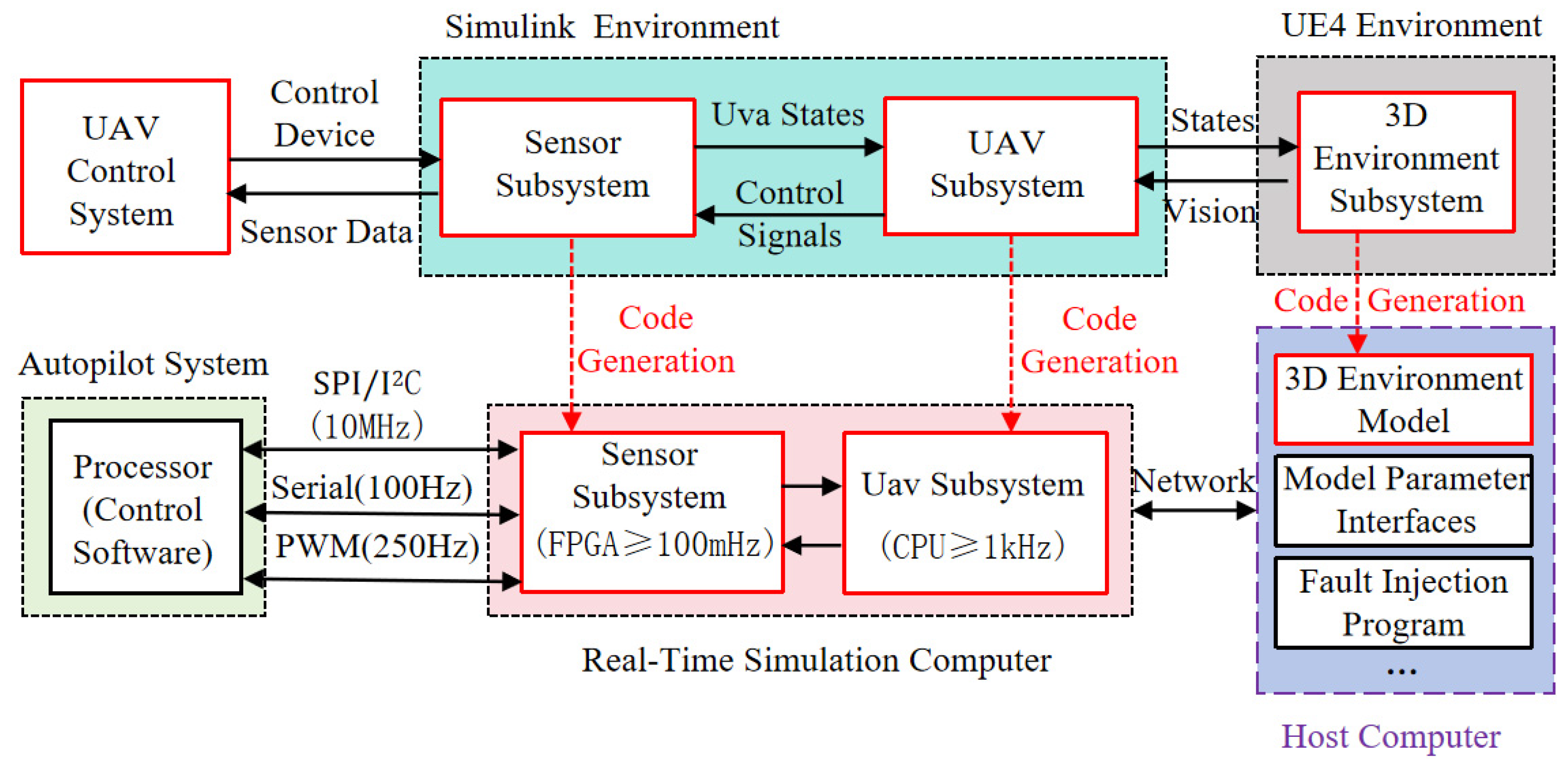
4.1. MBD-HIL UAV Development Strategy

There are two simulation methods for UAV automatic pilot systems: software-in-the-loop (SIL) simulation and HIL simulation. The SIL simulation model is used to quickly test control algorithms on computers, but the reliability of the simulation results is limited because the control algorithm does not run on the physical hardware of the rotary-wing logistics UAV. To improve the reliability of the simulation, in the HIL simulation experiment, the flight controller of the logistics UAVs and the real-time simulation computer work together to reflect the real operating environment of the control algorithm. The HIL simulation experiment works by connecting physical hardware devices with software platforms. The robust control algorithm of the logistics UAVs runs on the flight controller, and the sensor signals come from the real-time simulation computer, thus verifying the correctness of the hardware system and algorithm. In Figure 5, (a) shows the logistics UAV system in the real world; (b) shows the logistics UAV simulation model in the SIL running control algorithms on the same computer; and (c) demonstrates the operation principle of the HIL simulation experiment.
The HIL simulation experiment of the logistics UAVs uses the Pixhawk 4 flight controller as the hardware and Simulink as the software platform. The framework flowchart of the MBD-HIL method is shown in Figure 6. A simulation model of a rotor logistics UAV is developed in the Simulink environment. To obtain real-time rendering and realistic 3D flight scenes, the currently popular game development engine Unreal Engine 4 (UE4) version 4.22 [41] was chosen. Simulink and UE4 provide a modular and visual programming environment, which facilitates the MBD-HIL method.
In the HIL simulation experiment, the flight control program was executed on the Pixhawk 4 platform, and noise and offsets were introduced to simulate the measurement values of the GPS. Additionally, the UE4 engine was utilized to create a simulated external environment encompassing flight terrain and weather conditions, as depicted in Figure 7.
Following the completion of the SIL development, the code was deployed to the Pixhawk 4 flight controller utilizing the code generation and deployment framework depicted in Figure 8. The operating frequency of the attitude loop is 400 Hz, and the operating frequency of the position loop is 250 Hz. This is primarily determined by the speed of the PX4 processor. For the inner and outer loop control systems, the attitude loop operates at a higher frequency than the position loop because the inner loop requires a faster operating speed and higher response frequency.
To accurately simulate real flight conditions, three-dimensional gust disturbances were incorporated into the control block diagram. These disturbances were generated by combining sinusoidal and random signals, and their mathematical expression is presented below:
D = [ 1.8 + 0.1 sin ( t ) 1.8 + 0.1 sin ( t ) 1.4 + 0.075 sin ( t ) ] + [ d 1 d 2 d 3 ]
To incorporate the uncertainty of gust disturbances, random numbers are generated as follows: d i [ 1 , 1 ] and i = 1 , 2 , 3 .
Considering the extensive utilization of cascaded dual-loop PID controllers in open-source UAVs, a comparative analysis is conducted between the proposed algorithm and conventional cascaded dual-loop PID controllers.
Root Mean Squared Error (RMSE) is a metric used to measure the predictive accuracy of a forecasting model on continuous data. It quantifies the root mean square difference between predicted values and true values, indicating the average deviation between predicted and true values. In this paper, RMSE is used to quantitatively reflect the performance of the controller.

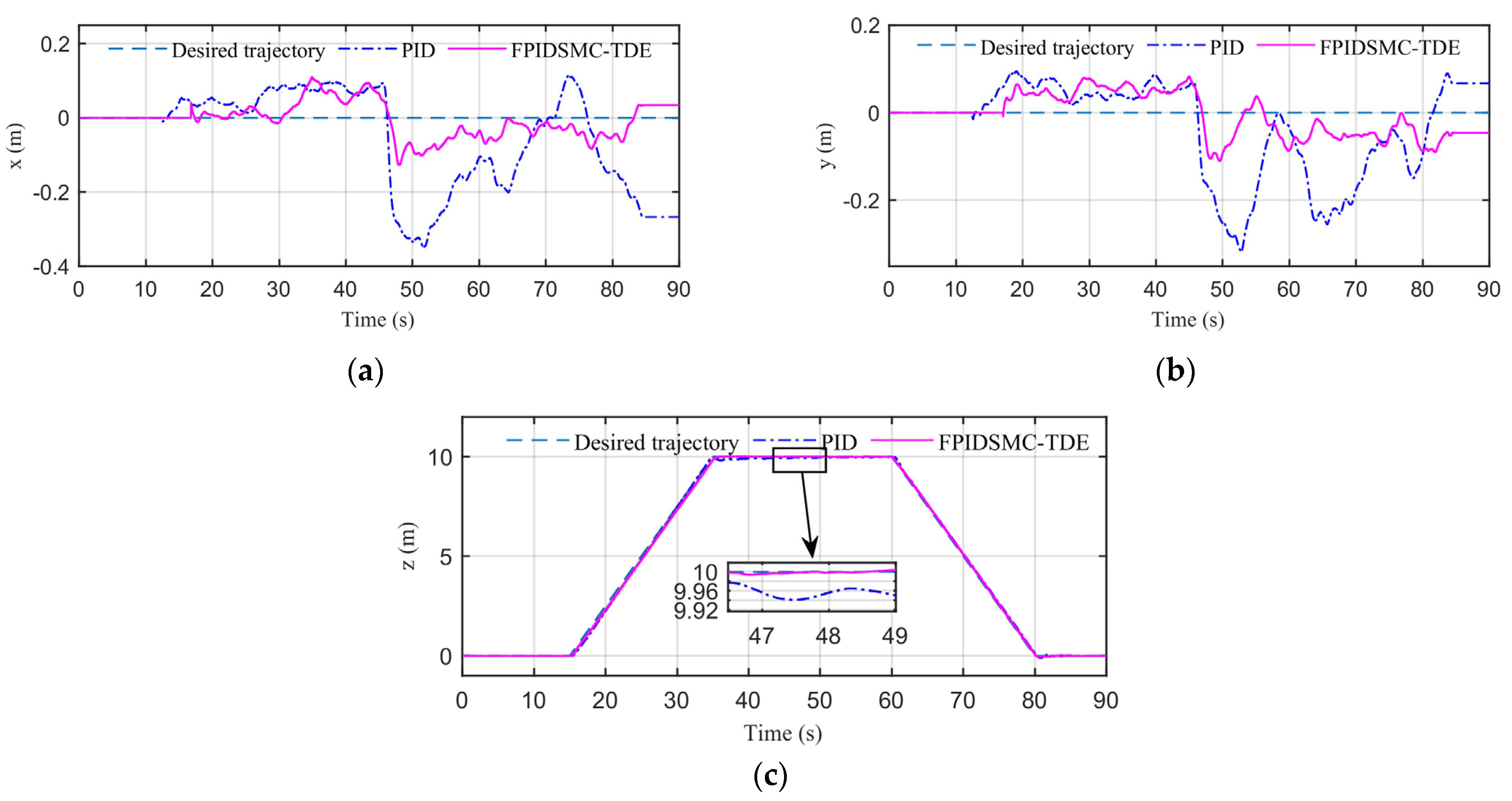
4.1.1. HIL for the Hovering Experiment

A hovering experiment of logistics UAVs was conducted to investigate their ability to maintain a stable position without drifting or oscillating during the hovering process, which reflects a stable performance. Figure 9 displays the displacement error curves in three directions during the hovering experiment of the logistics UAVs. When considering gust disturbances, the proposed strategy outperforms the conventional cascaded dual-loop PID controller in terms of generating a more stable control force for position control. This highlights the advantage of finite-time control in the attitude control loop, enabling a faster response to suppress the influence of gust disturbance on the system. Using cascade PID control, the RMSE values in the Xe, ye, and ze directions are 0.1431, 0.1128, and 6.5109, respectively. Using the proposed strategy, the RMSE in the Xe, ye, and ze directions are 0.0463, 0.0493, and 6.5107, respectively. The proposed position controller achieves higher control accuracy than does the cascaded dual-loop PID control because of the effect of the PID-type sliding mode surface.

4.1.2. HIL Experiment for the Crash Recovery

At an altitude of 15 m, the logistics UAV was placed in a hovering state and deliberately dropped from the air. After a 0.5 s simultaneous shutdown of all four motors, the motors were restarted by the controller, after which the operation of the propellers resumed. This process aimed to assess the UAV’s ability to recover stability after losing control and to evaluate the robustness of the control algorithm in extreme environments.
Following the 0.5 s shutdown, the rotorcraft logistics UAV attained a downward vertical speed of 5.33 m/s, resulting in a kinetic energy of 14.2 J. The displacement trajectory curve is depicted in Figure 10. In the vertical direction, using the proposed strategy, the UAV descended by 2.09 m from its pre-stabilized position. In contrast, the PID algorithm reduced the altitude by 2.14 m from the point at which the UAV falls before stabilizing. Furthermore, in the Xe and Ye directions, the proposed algorithm exhibited displacement errors of 0.155 m and 0.113 m, respectively, while the PID algorithm had displacement errors of 0.183 m and 0.225 m, respectively. In terms of time, the proposed algorithm facilitated the logistics UAV’s recovery to stability after a fall of 1.6 s, outperforming the PID controller for 4 s. Compared to the traditional PID algorithm, the proposed algorithm demonstrates improved robustness.

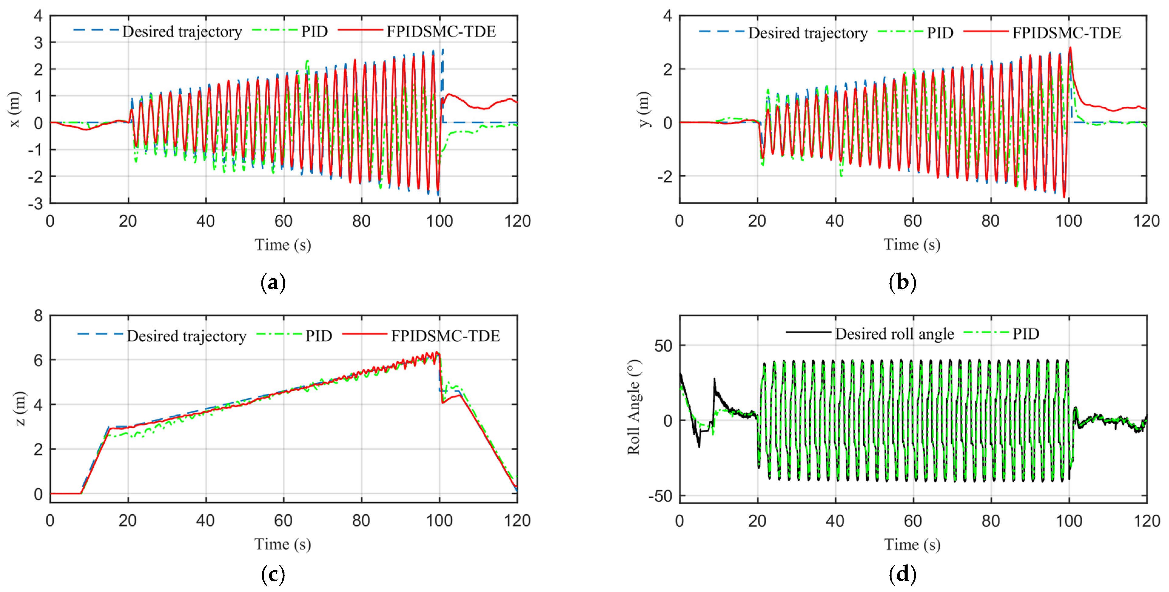
4.1.3. HIL for High Maneuverability Flight

In the scenario of high maneuverability flight, the expression for the flight trajectory of rotary-wing UAVs to track a clothoid curve is as follows:
{ x = 0.04 t cos ( 0.8 π t ) y = 0.04 t sin ( 0.8 π t )
As shown in Figure 11, upon reaching a certain altitude, the UAV begins to track a clothoid curve trajectory. As the curvature radius of the clothoid curve increases, the UAV gradually accelerates, resulting in a higher velocity. Examining the displacement error curve, it can be observed that the displacement error increases with an increasing curvature radius of the clothoid curve. Starting from a hovering state, the UAV completes 15 circular flights, reaching an instantaneous velocity of 14.76 m/s. This signifies the transition into a high-speed flight regime, where the aerodynamic drag disturbance imposed on the rotary-wing UAV reaches a magnitude of 5.77 N. As the velocity of the UAV continues to increase, the disturbance caused by aerodynamic drag progressively strengthens, leading to an increase in the displacement error. When the velocity of the rotary-wing UAV reaches 25.87 m/s, the flight radius no longer increases, indicating that the aircraft has reached its maximum speed limit. Using cascaded PID control, the RMSE values in roll, pitch, yaw, xe, ye, and ze directions are 13.3329, 14.2063, 22.9684, 0.6517, 0.8959, and 0.2458, respectively. In comparison, employing the proposed strategy results in RMSE values in roll, pitch, yaw, xe, ye, and ze directions of 4.2964, 3.7032, 13.9116, 0.3278, 0.2932, and 0.1375, respectively. The proposed strategy significantly improves the accuracy of attitude and position tracking.

4.2. In-Flight Experiments

This section aims to develop an autopilot for a logistics UAV using a model-based design with the MBD-HIL method and to perform in-flight experiments under extreme conditions to verify the effectiveness of the proposed strategy.
The MBD-HIL method is employed to deploy the algorithm on the Pixhawk 4 autopilot. The detailed hardware configuration of Pixhawk 4 includes the following components: MCU-STM32F427, sensors-MPU6000, MS5611, LSM303D, L3GD20H, and Ublox-M8N. The Pixhawk 4 autopilot system is widely recognized as the most prevalent and open-source autonomous control system for UAVs. Additionally, the Pixhawk 4 32-bit flight control unit (FCU) is equipped with an M9N GPS and a pair of 3DR radiotelemetry radios. Telemetry communication between the UAV’s MCU and the off-board controller is facilitated via the MavLink protocol, while real-time information access is made possible through the MAVROS interface.

4.2.1. The In-Flight Hover Experiment

The displacement error curves in three directions during the hovering experiment of the logistics UAVs are illustrated in Figure 12. A comparison between the PID controller and the proposed strategy reveals that the proposed strategy exhibits superior control accuracy in the in-flight hover experiment, yielding results comparable to those obtained with the HIL experiment. Despite the presence of slight wind disturbance in the outdoor flight environment, the FNTSM algorithm displays finite-time convergence characteristics, enabling a rapid response in the attitude loop and the effective suppression of external disturbances. This exemplifies the advantages of employing finite-time control in the attitude control loop, as it allows for a faster response to mitigate the impact of gust disturbances on the system. In the position loop, the integral term of the PID-type sliding mode surface effectively eliminates steady-state errors and enhances the position control accuracy of the controller. Using cascaded PID control, the RMSE values in Xe, ye, and ze directions are 0.1462, 0.0965, and 0.2228, respectively. In contrast, employing the proposed strategy yields RMSE values in Xe, ye, and ze directions of 0.0534, 0.0561, and 0.0772, respectively.

4.2.2. The Actual Flight Crash Experiment

The experimental scenario for the actual flight crash test is designed to closely mimic real-world conditions, with the UAV experiencing a free fall from a 5 m height for 0.5 s before stabilizing for hovering flight. Figure 13 shows the displacement curves in the Xe, Ye, and Ze axes during the crash test. It is evident that while the control precision of the proposed control strategy is marginally superior in the Xe and Ye directions, the overall performance difference between the two algorithms is minimal. In the Ze direction, both control strategies result in a similar descent height for the UAV. However, the PID algorithm exhibits a 2 m overshoot when the UAV ascends from its falling position to a height of 5 m. In contrast, the proposed control strategy demonstrates minimal overshoot, underscoring the robustness of the proposed algorithm.
To thoroughly investigate the self-rescue capability of the rotorcraft logistics UAV, various shutdown experiments were conducted during the actual flight crash test. It was observed that when all four motors were shut down for a duration of 0.75 s, the PID algorithm proved ineffective at achieving self-rescue. Likewise, when the shutdown duration was extended to 1 s, the proposed algorithm also failed to successfully execute self-rescue.

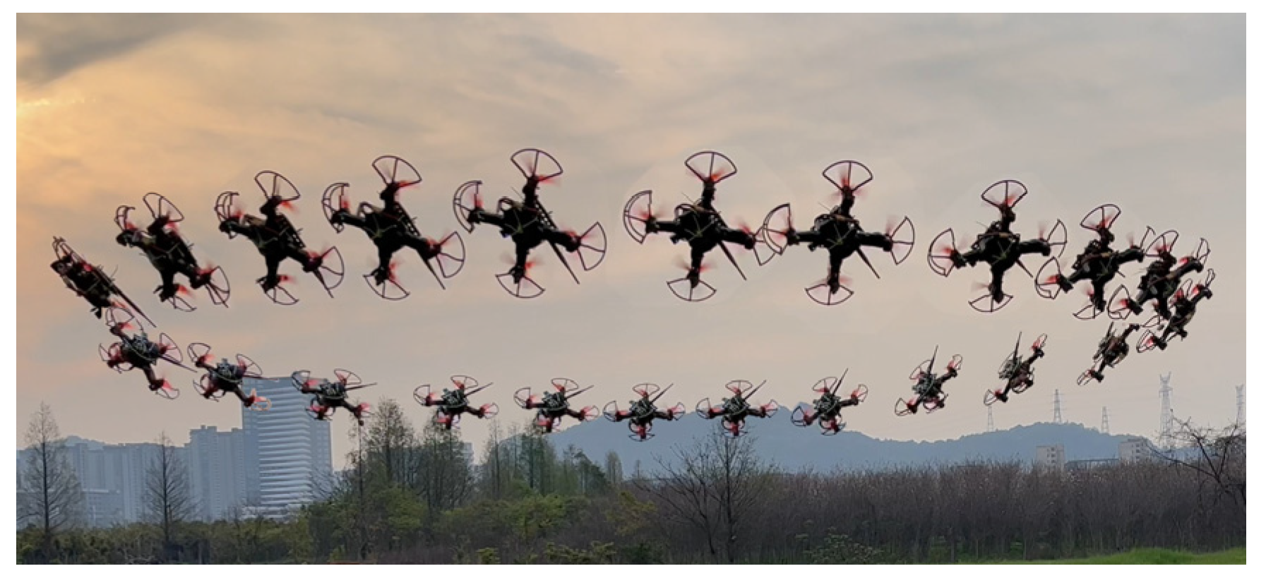
4.2.3. High Maneuverability Flight Field Experiment

Figure 14 displays the sequence diagram of the experimental flight maneuver. As shown in Figure 15, according to the displacement curve plots along the X- and Y-axes, after 40 s, the PID controller is no longer able to track the desired clothoid trajectory. In contrast, the proposed strategy is capable of accurately tracking clothoid trajectories. The rotary-wing drone performs circular flight at a fixed frequency, and as the radius increases, the UAV’s speed also increases. With the proposed strategy, the maximum speeds of the UAV in the Xe and Ye directions are 25.45 m/s and 25.53 m/s, respectively, with maximum accelerations of 15.89 m/s2 and 14.95 m/s2, respectively. Using the PID controller, the maximum speeds of the UAV in the Xe and Ye directions are 13.04 m/s and 13.2 m/s, respectively, with maximum accelerations of 9.7 m/s2 and 9.29 m/s2, respectively. It is evident that the proposed controller enables the UAV to achieve faster flight speeds and greater maneuverability.
As shown in Figure 15c, the desired trajectory in the Z-axis direction is a relatively simple linear trajectory. The PID controller exhibits greater fluctuations in tracking the desired trajectory, while the proposed control strategy maintains stable flight status before 60 s and experiences flutter during high-speed flight from 80 to 100 s. In comparison, the flutter effect of the PID controller is significantly stronger than that of the proposed control strategy. As shown in Figure 15d,e, under the influence of the proposed controller, the roll angle of the rotary-wing drone gradually increases, which is more in line with the need for a continuously increasing roll angle as the curvature radius of the clothoid curve changes. The maximum roll angle reaches 71°. Under PID control, the roll angle mainly varies between −40° and +40°, thereby restricting the increase in the flight speed of the UAV. Moreover, as shown in subplots (a) and (b), under the PID controller, the UAV can track the desired trajectory within the first four loops of the clothoid curve, but it is unable to track the desired trajectory thereafter due to speed constraints. Under cascaded PID control, the RMSE values in roll, pitch, yaw, xe, ye, and ze directions are 10.4032, 9.8000, 19.9750, 1.0539, 0.7705, and 0.2263, respectively. Utilizing the proposed strategy results in RMSE values in roll, pitch, yaw, xe, ye, and ze directions of 4.9413, 6.8863, 13.2600, 0.8319, 0.4035, and 0.1375, respectively. Similar to the results of the HIL experiment, the proposed strategy enhances the accuracy of attitude and position tracking.

5. Conclusions

To enhance the robustness of rotorcraft logistics UAVs, this paper proposes a cascaded dual-loop SMC strategy. The inner loop, devoted to attitude control, implements the FNTSM approach to achieve high-speed response characteristics. Moreover, the outer loop, which is responsible for position control, adopts a PID-type sliding mode surface to realize high-precision positioning. Addressing the challenge of unknown disturbances encountered during UAV flight, the proposed strategy utilizes the TDE technique to acquire aggregated unknown terms for the online estimation and real-time compensation of system dynamics. This approach efficiently reduces the gain coefficients of the SMC controller. The stability of the proposed strategy is analyzed through Lyapunov stability theory. Additionally, a model-based development approach tailored for hybrid twin-rotor logistics UAVs is developed to enhance development efficiency. Through scenarios including hover, crash, and high-mobility flight, both simulations and flight tests demonstrate that the proposed strategy exhibits superior maneuverability and higher motion tracking accuracy than does the PID algorithm. Due to the use of Euler angles to represent the attitude angles of the UAV, the proposed strategy cannot avoid the singularity issues of the attitude angles. In future work, quaternion representation will be employed to address the singularity issues of the attitude angles in the UAV.

Author Contributions

Conceptualization, S.Y. and P.C.; methodology, J.M.; software, W.H.; validation and data curation, H.W. and J.Z.; investigation, and formal analysis, X.L. and Y.Z.; funding acquisition, S.Y., J.M. and P.C. All authors have read and agreed to the published version of the manuscript.

Funding

This research was funded by the Wenzhou Scientific Research Project under Grant No. G20210045, Wenzhou Major Scientific Research Project under Grant No. ZGF2023057, Wenzhou Research Institute of the University of Chinese Academy of Sciences under Grants No. WIUCASQD2021009, and WIUCASSWCL21002, Wenzhou Key Scientific Research Project under Grant No. ZGF2023056.

Data Availability Statement

The data that support the findings of this study are available from the corresponding author upon reasonable request.

Acknowledgments

The authors gratefully acknowledge the assistance of these support agencies.

Conflicts of Interest

The authors declare no conflicts of interest.

References

  1. Zhai, D.; Wang, C.; Cao, H.; Garg, S.; Hassan, M.M.; AlQahtani, S.A. Deep neural network based UAV deployment and dynamic power control for 6G-Envisioned intelligent warehouse logistics system. Future Gener. Comput. Syst. 2022, 137, 164–172. [Google Scholar] [CrossRef]
  2. Eun, J.; Song, B.D.; Lee, S.; Lim, D.E. Mathematical investigation on the sustainability of UAV logistics. Sustainability 2019, 11, 5932. [Google Scholar] [CrossRef]
  3. Elmokadem, T.; Savkin, A.V. Towards fully autonomous UAVs: A survey. Sensors 2021, 21, 6223. [Google Scholar] [CrossRef] [PubMed]
  4. Song, B.D.; Park, K.; Kim, J. Persistent UAV delivery logistics: MILP formulation and efficient heuristic. Comput. Ind. Eng. 2018, 120, 418–428. [Google Scholar] [CrossRef]
  5. Yu, Y.; Guo, J.; Ahn, C.K.; Xiang, Z. Neural adaptive distributed formation control of nonlinear multi-UAVs with unmodeled dynamics. IEEE Trans. Neural Netw. Learn. Syst. 2022, 34, 9555–9561. [Google Scholar] [CrossRef] [PubMed]
  6. Garofano-Soldado, A.; Sanchez-Cuevas, P.J.; Heredia, G.; Ollero, A. Numerical-experimental evaluation and modelling of aerodynamic ground effect for small-scale tilted propellers at low Reynolds numbers. Aerosp. Sci. Technol. 2022, 126, 107625. [Google Scholar] [CrossRef]
  7. Pan, Y.; Chen, Q.; Zhang, N.; Li, Z.; Zhu, T.; Han, Q. Extending delivery range and decelerating battery aging of logistics UAVs using public buses. IEEE Trans. Mob. Comput. 2022, 22, 5280–5295. [Google Scholar] [CrossRef]
  8. Elmeseiry, N.; Alshaer, N.; Ismail, T. A detailed survey and future directions of unmanned aerial vehicles (uavs) with potential applications. Aerospace 2021, 8, 363. [Google Scholar] [CrossRef]
  9. Liang, S.; Zhang, S.; Huang, Y.; Zheng, X.; Cheng, J.; Wu, S. Data-driven fault diagnosis of FW-UAVs with consideration of multiple operation conditions. ISA Trans. 2022, 126, 472–485. [Google Scholar] [CrossRef]
  10. Bateman, F.; Noura, H.; Ouladsine, M. Fault diagnosis and fault-tolerant control strategy for the aerosonde UAV. IEEE Trans. Aerosp. Electron. Syst. 2011, 47, 2119–2137. [Google Scholar] [CrossRef]
  11. Zheng, E.H.; Xiong, J.J.; Luo, J.L. Second order sliding mode control for a quadrotor UAV. ISA Trans. 2014, 53, 1350–1356. [Google Scholar] [CrossRef] [PubMed]
  12. Xuan-Mung, N.; Hong, S.K. Improved altitude control algorithm for quadcopter unmanned aerial vehicles. Appl. Sci. 2019, 9, 2122. [Google Scholar] [CrossRef]
  13. Kazim, M.; Azar, A.T.; Koubaa, A.; Zaidi, A. Disturbance-rejection-based optimized robust adaptive controllers for UAVs. IEEE Syst. J. 2021, 15, 3097–3108. [Google Scholar] [CrossRef]
  14. Borase, R.P.; Maghade, D.K.; Sondkar, S.Y.; Pawar, S.N. A review of PID control, tuning methods and applications. Int. J. Dyn. Control 2021, 9, 818–827. [Google Scholar] [CrossRef]
  15. Meier, L.; Tanskanen, P.; Heng, L.; Lee, G.H.; Fraundorfer, F.; Pollefeys, M. PIXHAWK: A micro aerial vehicle design for autonomous flight using onboard computer vision. Auton. Robot. 2012, 33, 21–39. [Google Scholar] [CrossRef]
  16. Okasha, M.; Kralev, J.; Islam, M. Design and Experimental Comparison of PID, LQR and MPC Stabilizing Controllers for Parrot Mambo Mini-Drone. Aerospace 2022, 9, 298. [Google Scholar] [CrossRef]
  17. Kim, H.S.; Lee, K.; Joo, Y.H. Decentralized sampled-data fuzzy controller design for a VTOL UAV. J. Frankl. Inst. 2021, 358, 1888–1914. [Google Scholar] [CrossRef]
  18. Dumitrescu, C.; Ciotirnae, P.; Vizitiu, C. Fuzzy logic for intelligent control system using soft computing applications. Sensors 2021, 21, 2617. [Google Scholar] [CrossRef]
  19. Peitz, S.; Dellnitz, M. A survey of recent trends in multiobjective optimal control—Surrogate models, feedback control and objective reduction. Math. Comput. Appl. 2018, 23, 30. [Google Scholar] [CrossRef]
  20. Abdolrasol, M.G.; Hussain, S.S.; Ustun, T.S.; Sarker, M.R.; Hannan, M.A.; Mohamed, R.; Ali, J.A.; Mekhilef, S.; Milad, A. Artificial neural networks based optimization techniques: A review. Electronics 2021, 10, 2689. [Google Scholar] [CrossRef]
  21. Effati, S.; Pakdaman, M. Optimal control problem via neural networks. Neural Comput. Appl. 2013, 23, 2093–2100. [Google Scholar] [CrossRef]
  22. Xie, M.; Yu, S.; Lin, H.; Ma, J.; Wu, H. Improved sliding mode control with time delay estimation for motion tracking of cell puncture mechanism. IEEE Trans. Circuits Syst. I Regul. Pap. 2020, 67, 3199–3210. [Google Scholar] [CrossRef]
  23. Abro, G.E.M.; Zulkifli, S.A.B.; Asirvadam, V.S.; Ali, Z.A. Model-free-based single-dimension fuzzy SMC design for underactuated quadrotor UAV. Actuators 2021, 10, 191. [Google Scholar] [CrossRef]
  24. Wang, X.; van Kampen, E.-J.; Chu, Q. Quadrotor fault-tolerant incremental nonsingular terminal sliding mode control. Aerosp. Sci. Technol. 2019, 95, 105514. [Google Scholar] [CrossRef]
  25. Yu, S.; Xie, M.; Wu, H.; Ma, J.; Li, Y.; Gu, H. Composite proportional-integral sliding mode control with feedforward control for cell puncture mechanism with piezoelectric actuation. ISA Trans. 2022, 124, 427–435. [Google Scholar] [CrossRef]
  26. Lin, J.; Zheng, R.; Zhang, Y.; Feng, J.; Li, W.; Luo, K. CFHBA-PID algorithm: Dual-loop PID balancing robot attitude control algorithm based on complementary factor and honey badger algorithm. Sensors 2022, 22, 4492. [Google Scholar] [CrossRef]
  27. Maurya, P.; Morishita, H.M.; Pascoal, A.; Aguiar, A.P. A path-following controller for marine vehicles using a two-scale inner-outer loop approach. Sensors 2022, 22, 4293. [Google Scholar] [CrossRef] [PubMed]
  28. Yu, S.; Wu, H.; Xie, M.; Lin, H.; Ma, J. Precise robust motion control of cell puncture mechanism driven by piezoelectric actuators with fractional-order nonsingular terminal sliding mode control. Bio-Des. Manuf. 2020, 3, 410–426. [Google Scholar] [CrossRef]
  29. Khan MY, A.; Liu, H.; Habib, S.; Khan, D.; Yuan, X. Design and performance evaluation of a step-up DC–DC converter with dual loop controllers for two stages grid connected PV inverter. Sustainability 2022, 14, 811. [Google Scholar] [CrossRef]
  30. Abbas, W.K.A.; Vrabec, J. Cascaded dual-loop organic Rankine cycle with alkanes and low global warming potential refrigerants as working fluids. Energy Convers. Manag. 2021, 249, 114843. [Google Scholar] [CrossRef]
  31. Ma, J.; Xie, M.; Chen, P.; Yu, S.; Zhou, H. Motion tracking of a piezo-driven cell puncture mechanism using enhanced sliding mode control with neural network. Control Eng. Pract. 2023, 134, 105487. [Google Scholar] [CrossRef]
  32. Hou, Z.; Lu, P.; Tu, Z. Nonsingular terminal sliding mode control for a quadrotor UAV with a total rotor failure. Aerosp. Sci. Technol. 2020, 98, 105716. [Google Scholar] [CrossRef]
  33. Hassani, H.; Mansouri, A.; Ahaitouf, A. Performance evaluation of an improved non-singular sliding mode attitude control of a perturbed quadrotor: Experimental validation. J. Vib. Control 2023, 10775463231161848. [Google Scholar] [CrossRef]
  34. Xiao, L.; Ma, L.; Huang, X. Intelligent fractional-order integral sliding mode control for PMSM based on an improved cascade observer. Front. Inf. Technol. Electron. Eng. 2022, 23, 328–338. [Google Scholar] [CrossRef]
  35. Labbadi, M.; Cherkaoui, M. Novel robust super twisting integral sliding mode controller for a quadrotor under external disturbances. Int. J. Dyn. Control 2020, 8, 805–815. [Google Scholar] [CrossRef]
  36. Hu, J.; Wang, Z.; Liu, G.P. Delay compensation-based state estimation for time-varying complex networks with incomplete observations and dynamical bias. IEEE Trans. Cybern. 2021, 52, 12071–12083. [Google Scholar] [CrossRef] [PubMed]
  37. LaForest, L.; Hasheminasab, S.M.; Zhou, T.; Flatt, J.E.; Habib, A. New strategies for time delay estimation during system calibration for UAV-based GNSS/INS-assisted imaging systems. Remote Sens. 2019, 11, 1811. [Google Scholar] [CrossRef]
  38. Yu, S.; Yu, X.; Shirinzadeh, B.; Man, Z. Continuous finite-time control for robotic manipulators with terminal sliding mode. Automatica 2005, 41, 1957–1964. [Google Scholar] [CrossRef]
  39. Bullock, D.; Johnson, B.; Wells, R.B.; Kyte, M.; Li, Z. Hardware-in-the-loop simulation. Transp. Res. Part C Emerg. Technol. 2004, 12, 73–89. [Google Scholar] [CrossRef]
  40. Gaviani, G.; Gentile, G.; Stara, G.; Romagnoli, L.; Thomsen, T.; Ferrari, A. From conception to implementation: A model based design approach. IFAC Proc. Vol. 2004, 37, 29–34. [Google Scholar] [CrossRef]
  41. Zhao, Y.; Zhong, R.; Cui, L. Intelligent recognition of spacecraft components from photorealistic images based on Unreal Engine 4. Adv. Space Res. 2023, 71, 3761–3774. [Google Scholar] [CrossRef]
Figure 1. Schematic diagram of a logistics UAV.
Drones 08 00058 g001
Figure 2. Control block diagram of the position controller.
Drones 08 00058 g002
Figure 3. Control block diagram of the attitude controller.
Drones 08 00058 g003
Figure 4. Flight control strategy for logistic UAVs.
Drones 08 00058 g004
Figure 5. Experimental strategies for SIL, HIL, and flight testing for UAVs. (a) represents the signal transmission process in the Real Machine System, (b) is the functional composition of software-in-the-loop, and (c) is the information transmission process in hardware-in-the-loop.
Drones 08 00058 g005
Figure 6. The framework flowchart of the MBD-HIL method.
Drones 08 00058 g006
Figure 7. The simulation environment for UAVs was developed by leveraging the powerful UE4 virtual game engine.
Drones 08 00058 g007
Figure 8. The code generation and deployment framework based on MBD-HIL.
Drones 08 00058 g008
Figure 9. The displacement curve of the HIL for the hovering experiment. (a) In the Xe direction. (b) In the Ye direction. (c) In the Ze direction.
Drones 08 00058 g009
Figure 10. The tracking performance of the four motors in the hovering state when all of them simultaneously stop rotating and stay idle for 0.5 s. (a) In the Xe direction. (b) In the Ye direction. (c) In the Ze direction. (d) The UAV’s roll angle. (e) The UAV’s pitch angle. (f) The UAV’s yaw angle.
Drones 08 00058 g010
Figure 11. The trajectory curve of HIL for high maneuverability flight. (a) In the Xe direction. (b) In the Ye direction. (c) In the Ze direction. (d) The UAV’s roll angle using the PID controller. (e) The UAV’s roll angle using the proposed strategy. (f) The UAV’s pitch angle using the PID controller. (g) The UAV’s pitch angle using the proposed strategy. (h) The UAV’s yaw angle.
Drones 08 00058 g011
Figure 12. The displacement curve of the UAV during the actual flight hover experiment. (a) In the Xe direction. (b) In the Ye direction. (c) In the Ze direction.
Drones 08 00058 g012
Figure 13. The tracking performance of the UAV under hover mode with all four motors simultaneously shut down for 0.5 s. (a) In the Xe direction. (b) In the Ye direction. (c) In the Ze direction. (d) The UAV’s roll angle. (e) The UAV’s pitch angle. (f) The UAV’s yaw angle.
Drones 08 00058 g013
Figure 14. Sequence diagram of the experimental flight maneuver.
Drones 08 00058 g014
Figure 15. The trajectory curves of displacement and attitude angles in high-maneuvering flight. (a) In the Xe direction. (b) In the Ye direction. (c) In the Ze direction. (d) Roll angle trajectory curve using PID controller. (e) Roll angle trajectory curve using the proposed strategy. (f) Yaw angle trajectory curve using the proposed strategy.
Drones 08 00058 g015aDrones 08 00058 g015b
Table 1. Performance parameters of the UAVs.
ParameterValueParameterValue
Acceleration due to gravity g / ( m · s 2 )9.8 Moment   of   inertia   about   the   Z-axis   J z z / ( kg · m 2 )0.0104
UAV mass m/kg0.752 Drag   coefficient   k d / ( N · m · s 2 )0.0251
UAV arm length l/m0.125 Lift   coefficient   C T 0.0165
Moment   of   inertia   about   the   X-axis   J x x / ( kg · m 2 )0.0056 Resistance   coefficient   C d 0.0624
Moment   of   inertia   about   the   Y-axis   J y y / ( kg · m 2 )0.0056 Atmospheric   density   ρ 1.184
Disclaimer/Publisher’s Note: The statements, opinions and data contained in all publications are solely those of the individual author(s) and contributor(s) and not of MDPI and/or the editor(s). MDPI and/or the editor(s) disclaim responsibility for any injury to people or property resulting from any ideas, methods, instructions or products referred to in the content.

