A Drone-Powered Deep Learning Methodology for High Precision Remote Sensing in California’s Coastal Shrubs

Abstract

Wildland conservation efforts require accurate maps of plant species distribution across large spatial scales. High-resolution species mapping is difficult in diverse, dense plant communities, where extensive ground-based surveys are labor-intensive and risk damaging sensitive flora. High-resolution satellite imagery is available at scales needed for plant community conservation across large areas, but can be cost prohibitive and lack resolution to identify species. Deep learning analysis of drone-based imagery can aid in accurate classification of plant species in these communities across large regions. This study assessed whether drone-based imagery and deep learning modeling approaches could be used to map species in complex chaparral, coastal sage scrub, and oak woodland communities. We tested the effectiveness of random forest, support vector machine, and convolutional neural network (CNN) coupled with object-based image analysis (OBIA) for mapping in diverse shrublands. Our CNN + OBIA approach outperformed random forest and support vector machine methods to accurately identify tree and shrub species, vegetation gaps, and communities, even distinguishing two congeneric shrub species with similar morphological characteristics. Similar accuracies were attained when applied to neighboring sites. This work is key to the accurate species identification and large scale mapping needed for conservation research and monitoring in chaparral and other wildland plant communities. Uncertainty in model application is associated with less common species and intermixed canopies.

1. Introduction

Accurately mapping, assessing, and monitoring terrestrial vegetation is central to ecological and global change research [1]. Current methods are too costly or laborious to cover large areas. Remote sensing constructs images of the physical characteristics of an area by measuring its reflected and emitted radiation at a distance using special sensors [2]. Land cover of vegetation or other physical objects is commonly mapped using those remote sensing data to then construct classification models based on observed spectral and structural relationships, validating the land cover classifications based on a minimum mappable unit, determined by the available resolution of remotely sensed imagery. Satellites and aircraft provide valuable remote sensing data that are used in plant ecological research at regional and global scales but these systems are often limited in their capacity to provide images at the spatial, temporal, and spectral resolution needed to support research at finer ecological scales (i.e., species, populations) [3]. Affordability can also be an issue when researchers need high resolution satellite or aerial imagery across large areas [4]. Plant ecological research at finer scales often relies on approaches that use handheld sensor systems mounted to ground-mounted systems (e.g., poles, cranes, towers). The logistics of these ground-based measurements is often too time consuming and physically challenging to collect more than a limited number of samples or to apply them to more complex systems or over large geographic ranges. Additionally, such ground-based surveys are arduous, dangerous, and risk damaging sensitive flora in wildland habitats with diverse, dense plant communities [5]. Such challenges mean that ground-based sensing surveys in shrubland and forest communities are often very labor intensive, limited in spatiotemporal resolution, and prone to under-sampling.

Lightweight uncrewed aerial vehicles (UAVs), also called drones, are increasingly used as a remote-sensing platform in plant ecology. Their flexibility, reduced cost, reliability, autonomous capability, and high-resolution multispectral and structural data contribute to their usefulness in a variety of wildland systems at finer scales than spaceborne satellite or crewed aircraft imagery [6,7,8]. UAV data can also complement data collected using ground-based observations [9], satellites [10,11], and crewed aircraft surveys [12].

Advances in UAV hardware, coupled with developments in three-dimensional (3D) point cloud modeling of landscape structure using structure-from-motion (SfM) algorithms are providing an alternative to expensive LiDAR platforms for structural mapping [13]. Light detection and ranging (LiDAR) sensor systems are among the most accurate for measuring structural attributes at the stand and individual canopy levels [14,15], but the high equipment costs can make LiDAR sensors difficult to procure. Structure-from-motion (SfM) photogrammetry is a computer vision technique that constructs a 3D model from a set of overlapping two-dimensional (2D) digital photographs [16]. UAV-derived photogrammetric point clouds (PPCs) generated from drone photographs and structure-from-motion (SfM) algorithms provide an analogous three-dimensional (3D) structural measurement and are gaining popularity as a low-cost and accurate alternative to characterize ecologically relevant landscape structure, including the shapes and sizes of trees and shrubs [13,14]. SfM approaches coupled with spectral analysis have been used to identify tree species [17], assess small-scale tree canopy gaps [18], and estimate biomass in low-stature grassland vegetation [19].

Shrublands have gained attention because of the ecosystem services they provide [20,21,22,23], their increased vulnerability to global change (i.e., drought, fire, land use change) [24,25,26], and efforts to conserve and actively restore degraded shrublands in Mediterranean-type ecosystems [27,28,29], subtropical regions [30], and deserts [31]. This has spurred interest in applying UAV surveys in shrublands, but advances have been limited by the set of challenges related to quantifying the spatial distribution of species. Canopies in these ecosystems should be readily accessible given their low stature, but in many of the more diverse and spatially heterogeneous shrublands, dense and impenetrably overlapping canopies can limit physical access, increase risk to workers, and risk significant damage to sensitive flora. In more arid, spatially diffuse desert shrublands, mapping species distribution and quantifying biomass with satellite imagery is possible but with large uncertainties and logistically challenging field validation [32]. UAVs have been successfully used in sensitive shrubland habitats to map plant community structure [23,33], estimate biomass [34,35], map species distribution in highly dynamic environments [36], and augment the assessment of restoration success [37].

Chaparral shrublands are the dominant wildland vegetation type in Southern California and one of the most extensive ecosystems in California, with evergreen sclerophyllous shrubland cover making up approximately 9% of the state [38]. Satellite remote sensing has been used for vegetation classification in California coastal shrublands at the stand and community scale [39], for distinguishing perennial woody from herbaceous annual vegetation within a shrubland community [40], and for estimating aboveground biomass of dominant species [29]. Recent work utilized aerial imagery and LiDAR data from airplane flights to classify coastal scrub communities in terms of vegetation alliances and associated species with limited success due to interference from variable topography and available light conditions [41] No studies have explored the use of UAVs data and machine learning approaches to classify woody plant species at the level of individuals or patches in chaparral and scrub communities, as required to support ecological research.

Conventional land-cover classification maps are constructed from remotely sensed data using one of two general image analysis approaches: pixel-based classifiers and geographic object-based image analysis (OBIA) methods. Pixel-based classification approaches use spectral information associated with individual pixels, irrespective of their spatial distribution and land cover context to assign land cover classes. Pixel-based methods of image classification can further be separated into two classification approaches—unsupervised or supervised. Unsupervised pixel-based approaches group pixels into clusters based on their properties and classify each cluster with a land cover class independent of the researcher. Unsupervised pixel-based methods can be computationally faster and the automated nature of the approach does not require the researcher to provide contextual samples to constrain the classification process. Although faster, unsupervised pixel-based classification approaches often produce unsatisfactory results, especially when remote sensing data have a very high spatial resolution and objects of interest have high pixel heterogeneity—producing classifications that resemble what researchers term the “salt and pepper effect” [42].

Pixel-based approaches can also be supervised to control the relevance and accuracy of classification. In a supervised pixel-based classification approach, the researcher selects representative samples for each of the land cover classes of interest in an image. Samples are used to generate signature files that store the samples’ spectral information, and this information is used to make classifications by running a classification algorithm (e.g., support vector machine). With the increased availability of high-resolution remote sensing data, software developers and researchers have moved to the use of semi-automated OBIA classification procedures that analyze the spectral, spatial, and contextual properties of imagery pixels and use segmentation processes with iterative machine-learning algorithms to delineate objects in the landscape that can then be systematically classified. OBIA classification approaches group pixels into representative geometries based on a set of parameters designated by the researcher. These parameters are based on the scale, shape, texture, spectral properties, and geographic context of objects of interest [43]. The OBIA classification process is supervised, requiring input of samples that have been previously classified by humans to complete the classification process.

The use of artificial intelligence (AI) approaches for land-cover classification and mapping has a well-established history, particularly for satellite-based remote sensing [44]. Much of the success from AI in remote sensing has been in advancing the use of image processing and pattern recognition as improvements over conventional statistically-based procedures for classification of landscape features. Advances in graphics processors, classification algorithms, and the increased ability of artificial neural networks to accurately and efficiently classify imagery using multiple layers of features have driven a surge of interest in AI approaches to land cover classification. These deep learning approaches examine the intricate pixel-based structure in very large image datasets using a backpropagation algorithm that allows the machine to adjust its internal parameters to compute an accurate representation in each layer of its neural network based on the representation in the previous layer.

Research has determined that non-parametric decision tree machine learning algorithms, namely, random forest (RF) and support vector machine (SVM), are well suited to classify vegetation species using high-resolution multispectral and RGB UAV imagery [45]. The RF algorithm in particular is regarded as an effective classification modeling approach for remote sensing data in complex landscapes given its classification accuracy and high predictive stability compared to other approaches [46,47] given the ability to tune model parameters accurately and robustly [48], while decreasing the probability of an overfitted machine learning model [49]. Support vector machines (SVMs) are a machine learning tool that approach a higher rate of accuracy than random forest [50], but SVM classification accuracies can be reduced when the identification of target classes requires multiple high-resolution imagery bands.

One of the most successful deep learning classification approaches in vegetation remote sensing is the convolutional neural network (CNN) [51]. CNNs utilize computational models that are made up of multiple convolved layers that learn representations of data using multiple levels of mathematical abstraction [52]. The neural network is made up of ‘hidden-layers’ composed of two stages. In the first stage, the network completes a convolution of the previous layer at a particular kernel size and is able to store trainable weights. The second stage is a max-pooling stage, which aims to reduce the number of computational units by keeping only the most responsive kernel units derived from the first stage convolution. CNNs can consist of multiple convolutional and max pooling layers that end in a fully connected layer that receives input from all of the units from the previously hidden layer and has a decision unit for each class that the network can predict. In remote sensing applications, the most common form of CNNs uses a supervised learning approach and requires a series of labeled training input images containing a subject of interest, assigned by the researcher, that the computer can then use to assign importance to a variety of image attributes. Ultimately, the computer assigns learned weights that can be used to classify future imagery that was not part of the original training set. Two key advantages of CNN techniques are that it requires very little computational engineering and the approach can easily take advantage of the increased amount of available graphical processing power to process very high-resolution UAV data. CNNs achieve this by systematically reducing images into a data form that is easier to computationally process without losing features that are critical for accurate classification. Once the CNN is trained, it can be applied to classify an entire raster landscape. Applying the CNN model results in a spatially explicit probabilistic heat map for each classification. The assignment of a discrete classification to map regions can be achieved using fuzzy logic classifiers and a geographic object-based image analysis workflow (OBIA). CNN and OBIA approaches have demonstrated high classification performance on a variety of plant species classification applications in agriculture [53,54] and forestry [55,56]. Additionally, CNN approaches have been successful in detecting low-stature shrub species in a variety of plant communities [57,58,59,60]. Recently, CNN deep learning modeling has been combined with the OBIA classification approach, a process now termed CNN fusion (i.e., CNN + OBIA, CNN + GEOBIA, OCNN), with the aim of improving the overall accuracy of land cover classification by implementing an OBIA segmentation of CNN classification probability output [61,62].

A robust methodology for species-level classification in complex shrublands can greatly increase the possible spatial and temporal extent of species-level monitoring for conservation and restoration, species-specific stand-level health assessments, fire risk and fuel load assessment, and biomass and carbon sequestration modeling. We posit that a CNN machine learning approach coupled with OBIA can leverage the high-resolution multispectral and structural data from UAV flight surveys to efficiently and accurately classify shrub species canopy across landscapes. This study demonstrates how shrub and tree species in spatially heterogeneous stands of chaparral, coastal sage scrub, and oak woodland can be accurately classified and mapped using drone-based multispectral imagery and a CNN + OBIA supervised machine learning classification approach.

2. Materials and Methods

2.1. Study Area

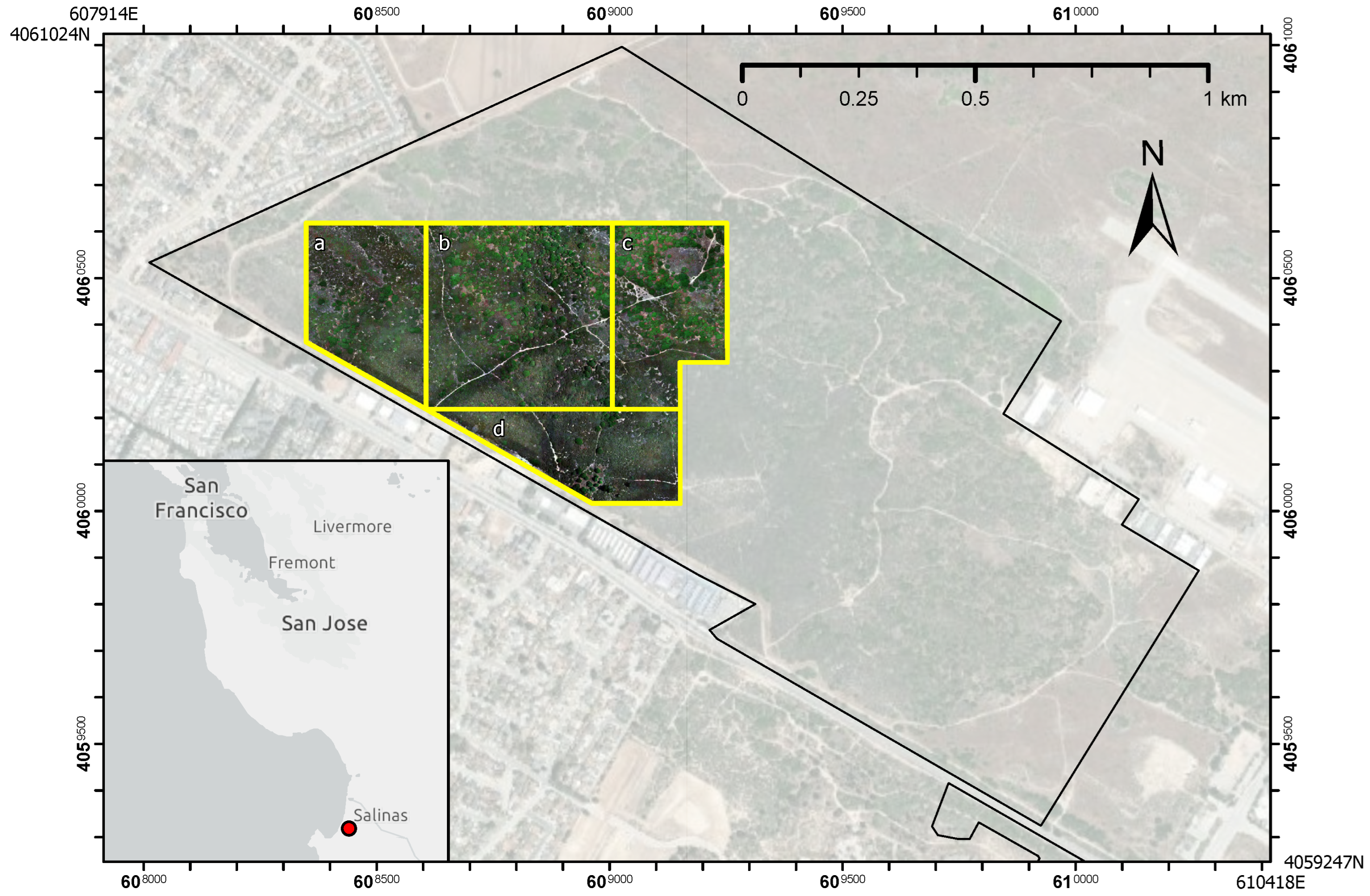
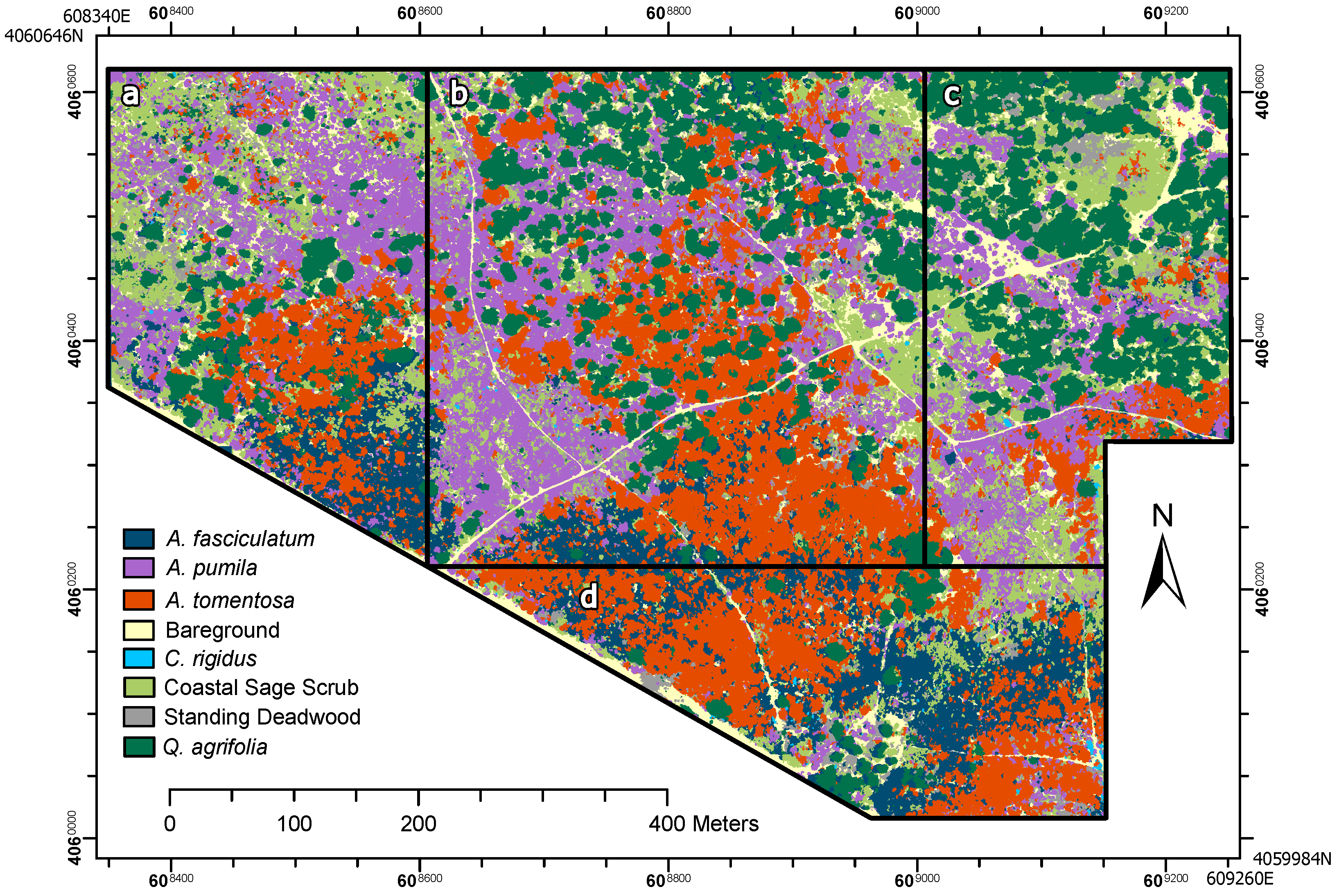
All research occurred on the 246-ha University California, Santa Cruz—Fort Ord Natural Reserve (UCSC-FONR) (Figure 1). The UCSC-FONR is located approximately 129 km south of San Francisco, CA, along the Monterey Bay and bordered by the city of Marina. This coastal parcel includes an abundance of low-growing shrublands among accessible rolling terrain (96 ha), ranging in elevation between 21 and 58 m above mean sea level. 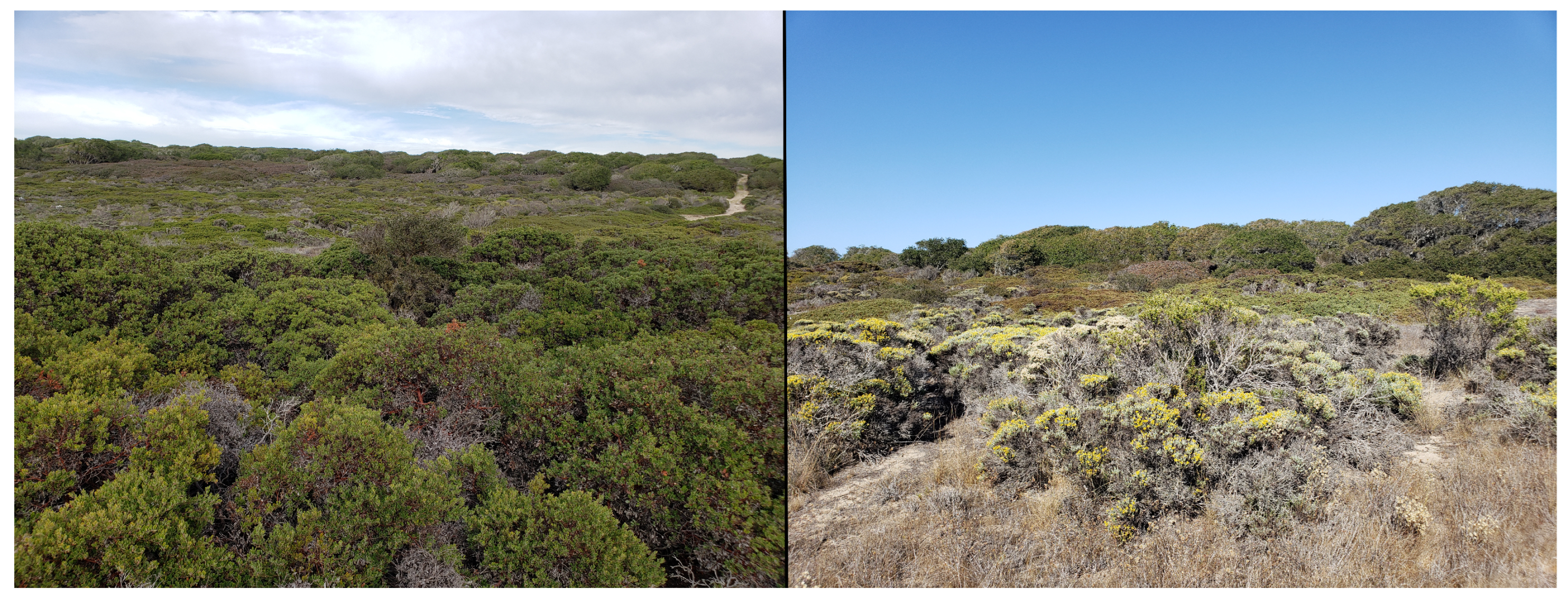We focused on a 40.7-ha area in the northwestern region of the reserve that includes a mosaic of three woody plant dominated coastal plant communities typical of the semi-arid coastal Mediterranean-type ecosystems of central California: maritime chaparral, coastal sage scrub, and coastal live oak woodland (Figure 2).

Maritime chaparral is a plant community found along the central California coastline and is characterized by sclerophyllous shrub species with hard, waxy-cuticle leaves. Dominant taxa in this community include manzanita species (Arctostaphylos tomentosa and A. pumila), chamise (Adenostoma fasciculatum), and a rare California lilac (Ceanothus rigidus). Coastal sage scrub is characterized by its drought-deciduous aromatic shrub species adapted to coastal lowlands in Mediterranean climate regions. Species associated with coastal sage scrub include California sagebrush (Artemisia californica), black sage (Salvia mellifera), coyote bush (Baccharis pilularis), and mock heather (Ericameria ericoides). Monotypic stands of coast oak woodlands (Quercus agrifolia) are surrounded by stands of maritime chaparral and coastal sage scrub. Some species are found in multiple plant communities (e.g., poison oak, Toxicodendron diversilobum) and several species can be intermixed at small scale. Four sites were determined based on the dominance of 10 of the 53 woody plant species known to occur in the region (

Table 1. Summary of the dominant woody plant species in the study sites and their associated plant communities. Arctostaphylos tomentosa ssp. tomentosa is referred to as A. tomentosa throughout this manuscript. Some species are known to inhabit all communities (e.g., T. diversilobum) and some coastal sage scrub species are known to encroach into mixed chaparral and coastal sage scrub.

Species	Common Name	Plant Communities
Adenostoma fasciculatum	Chamise	Maritime Chaparral
Arctostaphylos pumila	Sandmat Manzanita
Arctostaphylos tomentosa	Woolyleaf Manzanita
Ceanothus rigidus	Monterey Ceanothus
Artemisia californica	California Sage	Coastal Sage Scrub
Baccharis pilularis	Coyote Brush
Ericameria ericoides	Mock Heather
Salvia mellifera	Black Sage
Toxicodendron diversilobum	Poison Oak
Quercus agrifolia	Coast Live Oak	Oak Woodland

).

2.2. UAV Data Collection

UAV flight data were acquired in Summer 2021 (23 July 2021–24 July 2021), under high cloudy overcast skies, no fog, and light winds (2–5 km/h). We conducted five flight surveys ranging in area from 5 to 9 ha (Figure 1) All flights were approximately 30 min in duration and conducted near solar noon (11:00–13:00 PDT). Overcast conditions were ideal for limiting shadows created by taller neighboring vegetation that tend to obscure lower growing vegetation. All automated flight operations were planned and executed using DJI Pilot (v2.3.1.5) software as single pass grid flight patterns with 80% frontlap and at least 80% sidelap at a constant altitude of 60 m above the terrain to ensure the desired ground sampling distance (GSD; the distance between the centroids of two adjacent pixels measured on the ground). All flights were conducted by Section 107 FAA licensed pilots and in accordance with all federal, state, and local laws and regulations as well as all UC policies regarding small uncrewed aircraft system (sUAS) operation (UC-RK-18-0377).

A DJI Matrice 210 RTK V2 Pro quadcopter (DJI, Shenzhen, China) with approximately 30 min of flight autonomy was equipped with dual gimbals to accommodate two sensor systems capable of maximizing ground sampling distance (GSD) while capturing high-resolution narrow spectral band reflectance data. A Zenmuse X7 24 mm RGB camera with F2.8 leaf shutter aspheric lens captured high resolution imagery (GSD: 1 cm/pixel, 24 MP resolution) and was used in the generation of topographic rasters. The DJI Zenmuse X7 camera was connected to the onboard RTK-GNNS positioning system and WiFi connected to a DJI D-RTK Mobile Station which served as a high-precision GNSS ground receiver, providing real-time differential corrections of imagery position with centimeter-level positioning accuracy. The use of RTK correction negated the need for including ground control points in the sites. A MicaSense Altum multispectral sensor (MicaSense, Seattle, WA) collected calibrated narrow spectral band reflectance data at blue (455–495 nm), green (540–580 nm), red (658–678 nm), red edge (707–727 nm), and near infrared (800–880 nm) at GSD 2.5 cm/pixel. The RTK system was not compatible with logging positioning information to two image sensors so we used the MicaSense Altum sensor’s integrated GPS to record image positioning and later georeferenced Altum multispectral rasters to the reference RTK-collected Zenmuse X7 RGB data.

2.3. UAV Image Processing

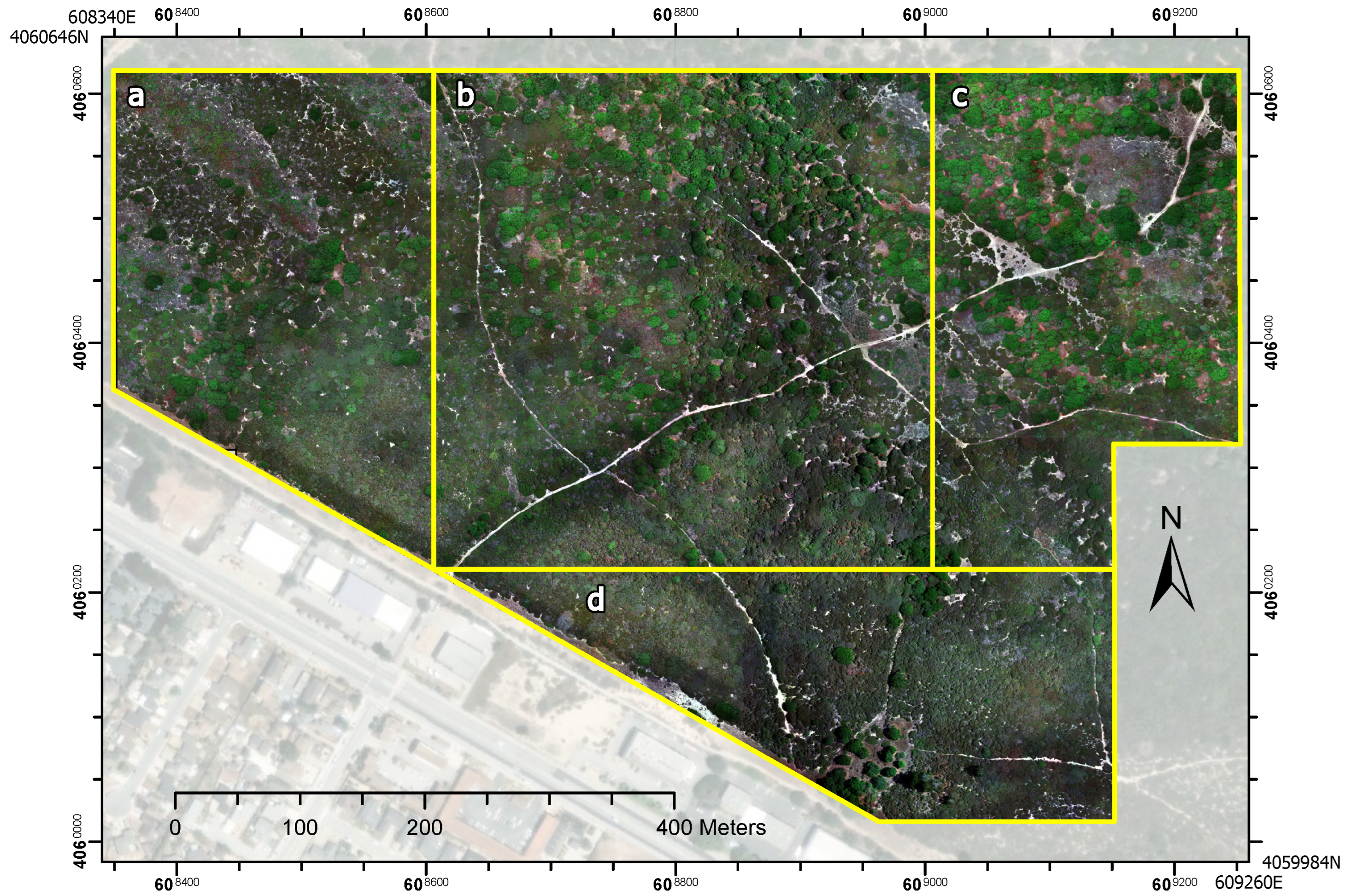
UAV imagery was photogrammetrically processed using Pix4DMapper Pro (v4.6.4) software (Pix4D SA, Lausanne, Switzerland) to generate multispectral orthomosaic and topographic rasters. An orthomosaic raster is an image generated from a mosaic of multiple georeferenced overhead images corrected for perspective and scale. Additional orthorectification of the multispectral raster to the reference Zenmuse X7 imagery was completed using the Auto Georeferencing function in ArcGIS Pro (v3.0.0, ESRI 2022). The Auto Georeferencing function in ArcGIS Pro requires two rasters with similar band structure and automates the selection of georeferencing control points that can be exported and used to georectify additional reflectance rasters. We generated an RGB composite orthomosaic raster from the Zenmuse X7 and Altum data and georeferenced the Altum RGB raster dataset to the X7 RGB raster dataset and exported the control points generated by the auto georeferencing function. These control points were used to georectify the remaining calibrated near-infrared and near-infrared edge reflectance rasters generated from the Altum Micasense sensor.

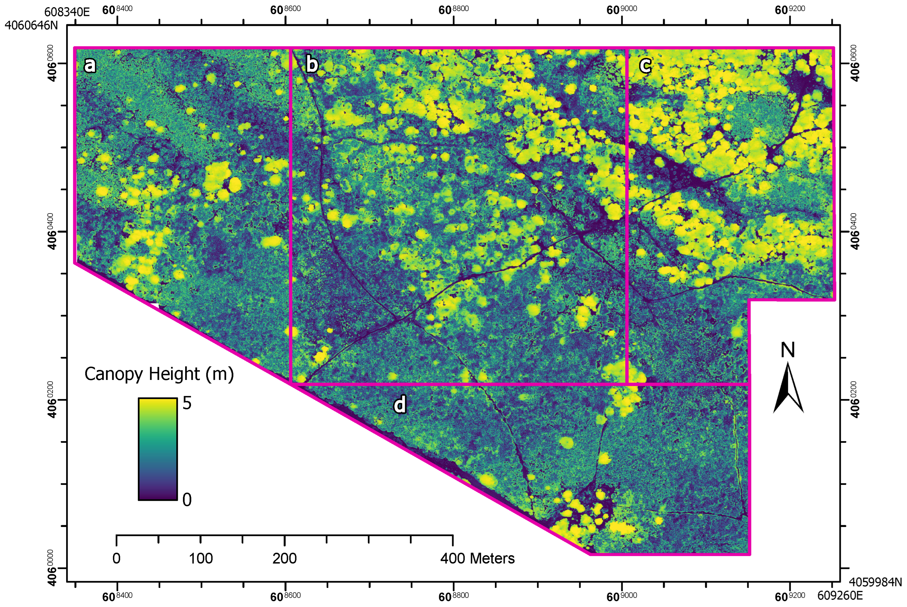
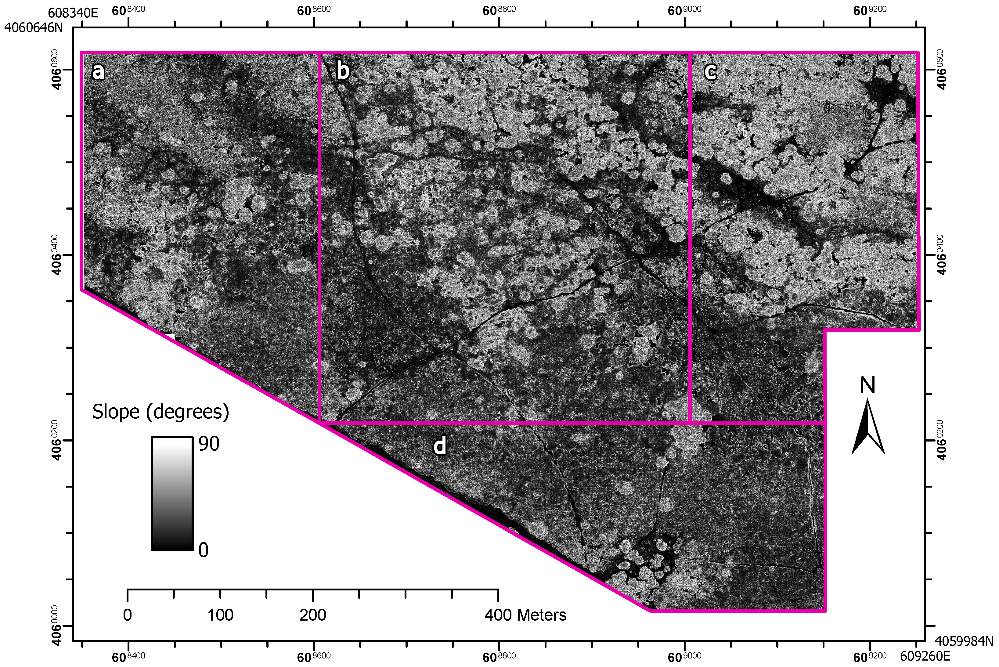
Topographic rasters included digital surface models (DSM) and digital terrain models (DTM) generated from Zenmuse X7 imagery and rendered point cloud data. DSM raster generation utilized a point cloud densification workflow with optimization at ½ image size and an inverse distance weighting algorithm application. DTM raster generation was achieved using a point cloud classification algorithm and Gaussian averaging producing a terrain model with lower resolution (5 cm/pixel). We used QGIS (v3.20.1-Odense) to generate a vegetation canopy height model from the normalized digital surface model (nDSM) by taking the arithmetic difference between the DSM and DTM raster values. We also calculated the slope values as a raster from the resulting nDSM. The percent slope model showed the maximum rate of elevation change between each cell and its neighbors calculated as the angle of inclination to the horizontal. Percent slope can be used to find the borders of overlapping tree canopies and gaps [17] and may support distinguishing between shrub species that have overlapping canopies as well as gaps in canopy. The slope raster was generated using the GDAL DEM utility in QGIS. All raster products were exported as 32-bit and 8-bit GeoTIFF format with WGS 84 / UTM zone 10N (EGM 96 Geoid) projection. A 64-bit Windows 10 PC equipped with an Intel^® Core™ i9-10900KF CPU at 3.70 GHz, 32 GB RAM, and an NVIDIA GeForce RTX 3060 graphics processor was used for all photogrammetric processing and machine learning modeling.

Flight Imagery

We successfully generated a multispectral orthomosaic (2.5 cm/pixel; Figure 3), nDSM (5 cm/pixel; Figure 4), and a slope raster (Figure 5) for the entire research site (40.7 ha).

2.4. Field Sampling

Between Summer 2021 and Summer 2022, we completed extensive ground surveys of woody vegetation across the four study sites. During the year-long period of surveys, we did not find any significant changes in the spatial distributions of the vegetation alliances and shrub species. Given the dense, often impenetrable canopies, we opted for a plotless sampling technique over transect or quadrat sampling methods. Previous surveys of the entire natural reserve have documented the presence of 53 woody plant species with dominance by 10 species. To acquire ground positions of woody plant species, we uploaded an 8-bit version of the high-resolution X7 RGB orthomosaic imagery from UAV flights to an Android tablet mobile device and accessed imagery in the field using the open-source GIS plugin QField [63]. The QField interface was configured in QGIS Desktop to include a data collection form that allowed field technicians to efficiently collect GPS point data on the position of woody plant species by referencing imagery in real time relative to their current ground position. GPS point data were collected for areas that were distinguishable in the imagery, larger than 0.5 m², and consisting of a single live species, bareground, or standing deadwood. Technicians recorded cover type and ensured that survey points were separated by distances of at least 3 m. All geodata were synchronized via the QField plugin in QGIS Desktop and stored in shapefile format.

We had a primary research interest in identifying individual species within the maritime chaparral plant community. We did not consolidate these species into a single classification category given management interests aimed at mapping the species distributions, assessing plant health, and estimating fuel loadings in the future. Manzanita, Ceanothus, and Chamise have very different fire-related characteristics [64]. To facilitate the focus on classification of those maritime chaparral species, we lumped all the species comprising the coastal sage scrub community into a single broad category; this eliminated the need for additional algorithms for deeper species-level classification. Creating this broader coastal sage scrub category also tested the ability of machine learning approaches to classify a group with high spectral variability at the same time as species-specific classifications with lower spectral variability.

2.5. Classification Modeling Development

We evaluated three OBIA integrated classifier methods: random forest (RF), support vector machine (SVM), and a deep learning convolutional neural networks (CNN) approach. All classifier methods were developed and applied into an object-based image analysis (OBIA) framework using eCognition Developer (v. 10.2, Trimble Germany GmbH, Munich, Germany). eCognition Developer is a development environment designed specifically to combine machine learning approaches with object-based image analysis through analysis workflows called rule sets. Two key advantages of this approach are (1) CNN integration based on Google’s TensorFlow API and (2) the ability to utilize the same OBIA landscape segmentation algorithms across the three classifier methods.

2.6. Image Sampling

In order to generate training and testing sample patches, survey points in the 16-ha training region (Figure 1) were randomly assigned to 70% training and 30% testing groups and labeled by membership to one of eight classification groups: A. fasciculatum, A. pumila, A. tomentosa, C. rigidus, Q. agrifolia, a Coastal Sage Scrub group, Deadwood, and Bareground. Survey points with distances to the raster scene border of less than 12 pixels were not used to generate samples. Samples were generated by rendering a square polygon buffer around ground survey points with sides of 0.6 m (0.36 m²) ground sampling distance (GSD), corresponding to 24 × 24 pixels image space, where each pixel represents 2.5 cm GSD. Samples were extracted from 8-bit multispectral rasters (i.e., red, green, blue, near-infrared (NIR), and near-infrared edge (NIRe)). Deep learning methods require thousands of training samples and this is often achieved by systematically rotating the scene orientation that sample patches are extracted from. This method can also rectify problems associated with the influence of shadow orientations. We used eCognition Developer (v. 10.2, Trimble Germany GmbH, Munich, Germany) to create a fully automated process that rotates the raster imagery at an interval of 30-degrees, extracts 1000 samples, and repeats the process a total of 12 times. The process generates 12,000 samples per class and a total of 96,000 samples across the eight cover classes.

Our convolutional neural network architecture began with random initial weights and received sample patches from the five multispectral image layers as training inputs with the goal of generating a probabilistic heat map of cover classes as an output. The model consists of two batch normalized hidden layers. In the first hidden layer, imagery is convoluted with a kernel size of 3 × 3 pixels and assigned to 40 feature maps without max pooling. In the second fully connected hidden layer, results from the first hidden layer are further convoluted using a 3 × 3 kernel size and assigned to 20 feature maps. Our CNN model consists of only the two hidden layers with no max pooling layers included. Max pooling is a method of reducing the pixel dimensions of the image thereby speeding processing time. CNN training was initiated by randomly shuffling training data and learning occurred at a rate of 0.0001 with 8000 training steps, and a sample batch size of 100 images. Learning rate defines the amount by which weights are adjusted in each iteration of the statistical gradient descent optimization.

2.7. CNN Application and OBIA Classification

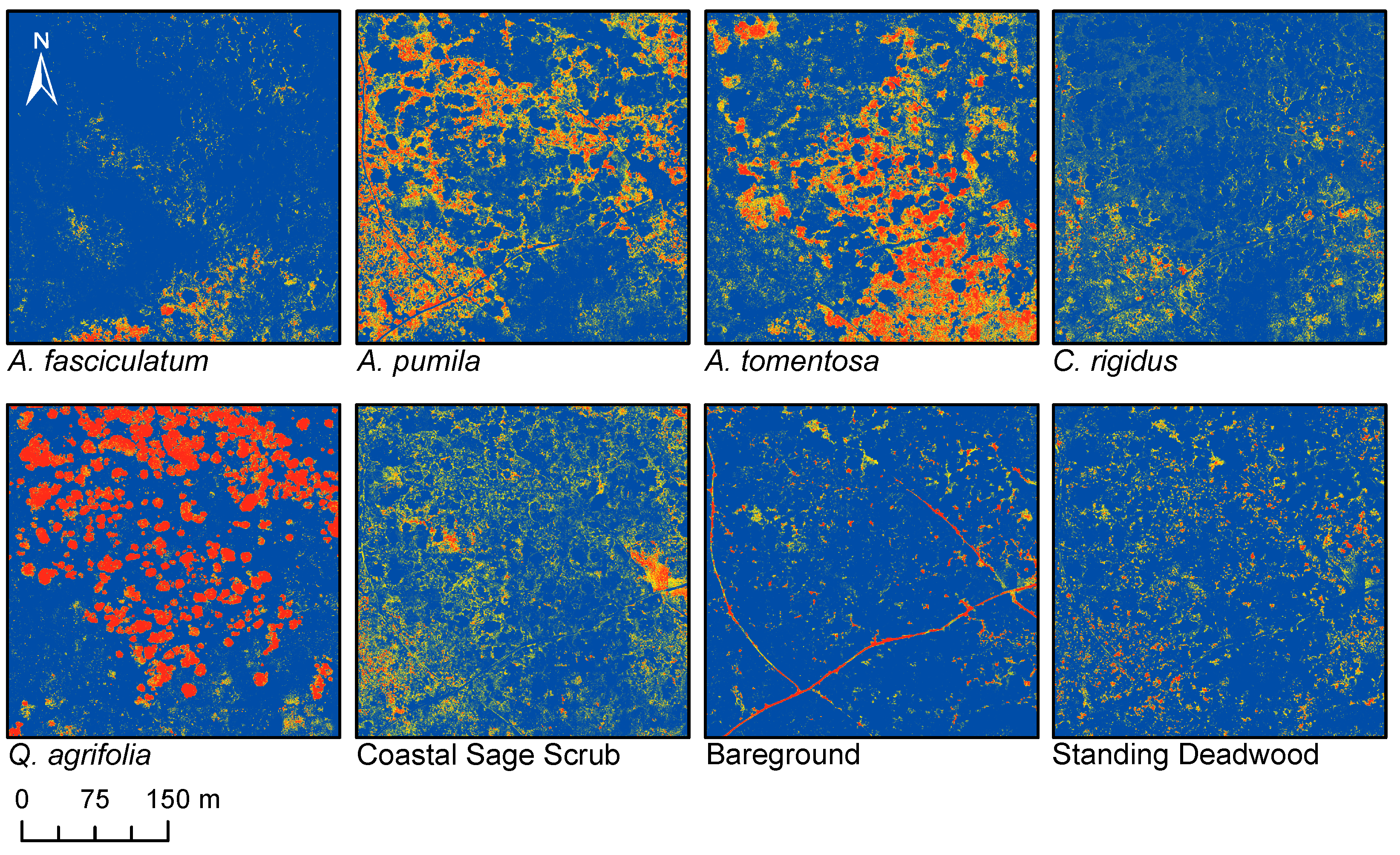
Once the CNN model was trained using training samples, we applied the model to the entire 16-ha training site and to the neighboring application sites. For each of the cover classes, we generated a separate raster heat map representing the probability that each pixel has membership within the cover classes (Figure 6).

2.8. Segmentation

Multiresolution segmentation, or MRS, is a widely used segmentation approach for OBIA classification with very-high-resolution (VHR) imagery [65]. We used the MRS algorithm in eCognition Developer (v. 10.2, Trimble Germany GmbH, Munich, Germany) to generate a segmentation vector layer for objectbased image classification. Multiresolution segmentation implements a method of segmentation known as region growing that iteratively merges neighboring regions with similar spectral and spatial heterogeneity based on thresholds defined by the researchers (Blaschke et al., 2004). Our segmentation process utilized the multispectral orthomosaic, canopy height (nDSM), and slope model as inputs with weightings assigned through trial and error as multispectral (4), canopy height (2), and slope (1). Segmentation parameters were set to a scale of 80, shape of 0.2, and compactness of 0.6.

Next, image segmentations were classified by generating a class hierarchy based on fuzzy logic membership using eCognition Developer 10.2. Each feature class in the classification hierarchy contained a class description consisting of a set of fuzzy logic membership functions that evaluated the specific probabilistic features of the individual heat maps generated from the CNN. We defined all of the fuzzy sets by linear membership functions that identified a soft fuzzy classifier that uses a degree of membership probability to express an object’s assignment to a class. The membership values range from 0.0 to 1.0, where 1.0 represents full membership to a feature class and 0.0 represents absolute non-membership. One advantage of these soft fuzzy logic methods lies in their ability to quantify uncertainties about the descriptions of feature classes and assign membership to a class based on the degree of uncertainty of membership in other classes. For this study, all membership functions varied between 0 and 1, except for C. rigidus, which was assigned a heat map probability threshold for classification that began at 0.85 instead of zero. This threshold was based on expert knowledge of where rare C. rigidus is actually located in the landscape and was determined by trial and error to accurately identify the species and reduce false-positive classification.

To assess accuracy during model development in the 16-ha training site, 30% of the randomly selected ground survey points were used to assign segmentation polygons as test classification polygons. If multiple ground survey test points of the same classification type were together in a test segmentation polygon, then we deleted test points so that only a single ground survey test point was associated with each testing segmentation polygon. Prior to testing we also ensured that training ground survey points were not within polygons that were assigned as test segmentation polygons. The overall impact of this process reduced the proportion of testing points by 1–2% per class and reduced the overall number of testing points total by 11% (

Table 2. Number of ground survey points collected at each site.

		Training Site			Application Site
Group	Species	Training	Testing	Corrected Testing	1	2	3
Chaparral	A. fasciculatum	174	74	67	244	9	303
	A. pumila	1545	662	562	387	492	247
	A. tomentosa	1065	457	369	295	218	573
	C. rigidus	162	69	64	16	87	33
Sage Scrub	A. californica	20	9	9	17	8	14
	B. pilularis	84	36	34	48	31	23
	E. ericoides	286	123	119	69	91	36
	S. mellifera	102	44	42	62	16	39
	T. diversilobum	35	15	14	30	57	18
Woodland	Q. agrifolia	913	392	376	186	306	82
Gaps		226	97	90	94	83	78
Bareground		340	146	136	70	112	72
	Total	4952	2124	1882	1518	1510	1518

).

2.9. Accuracy Assessment

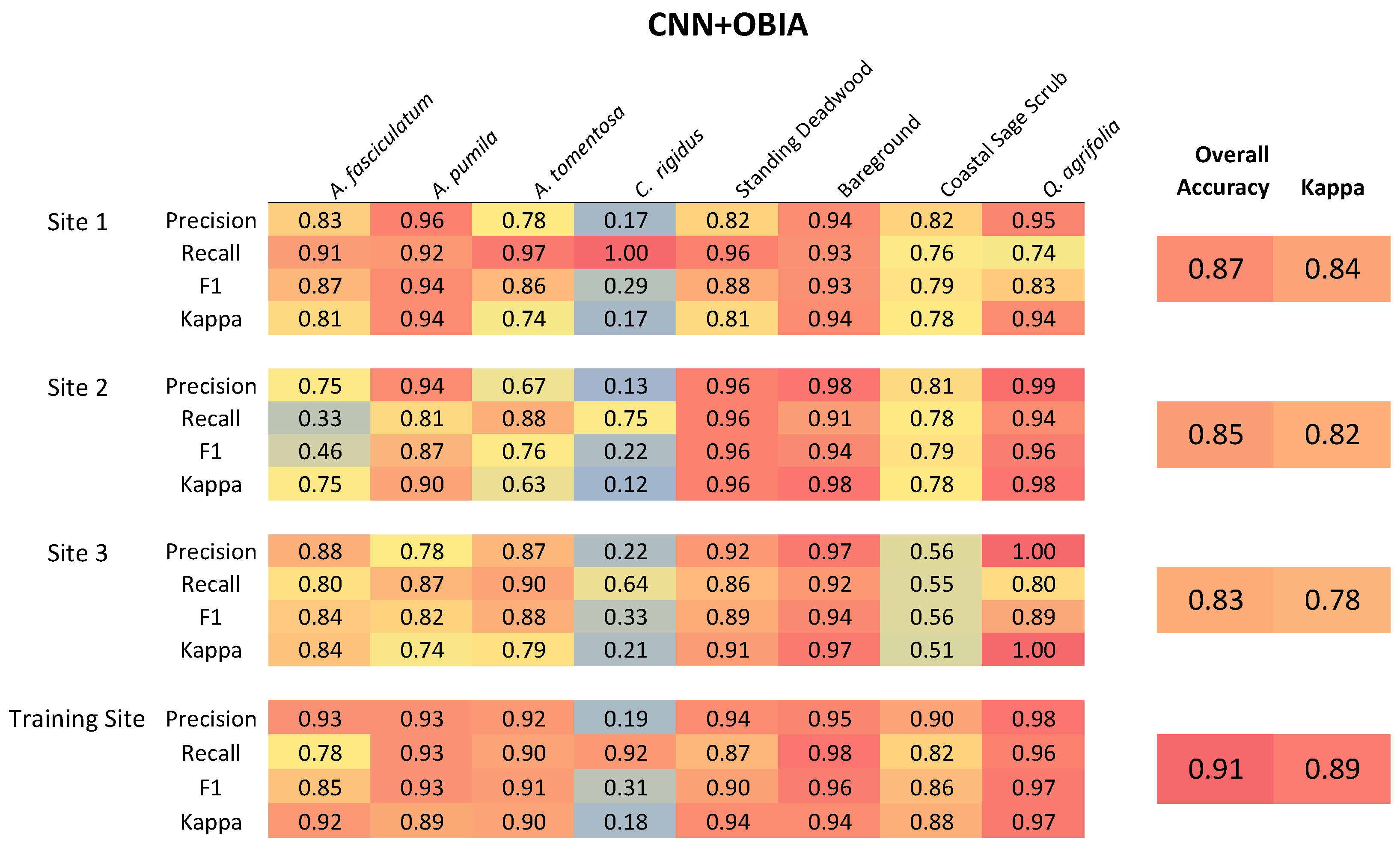
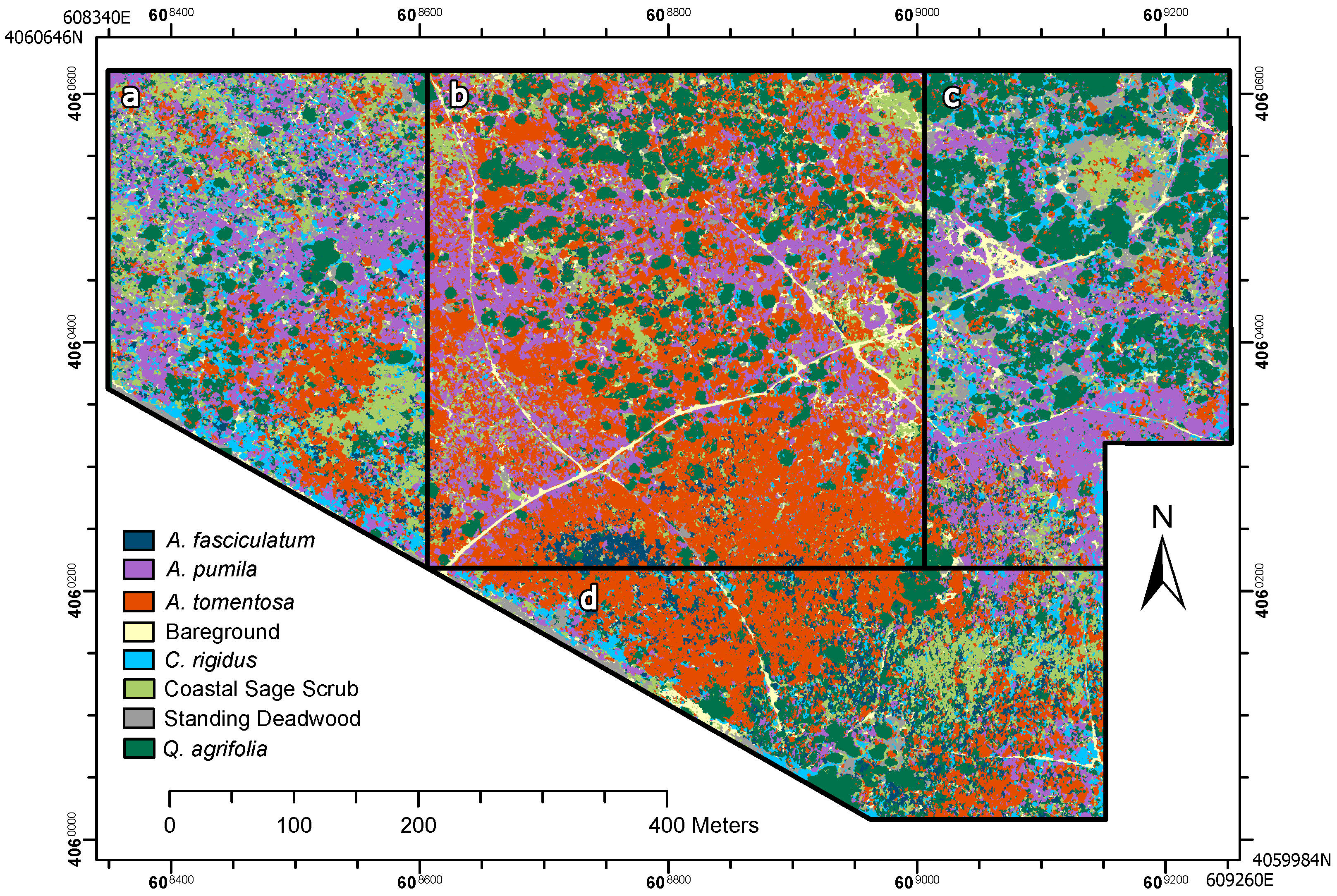
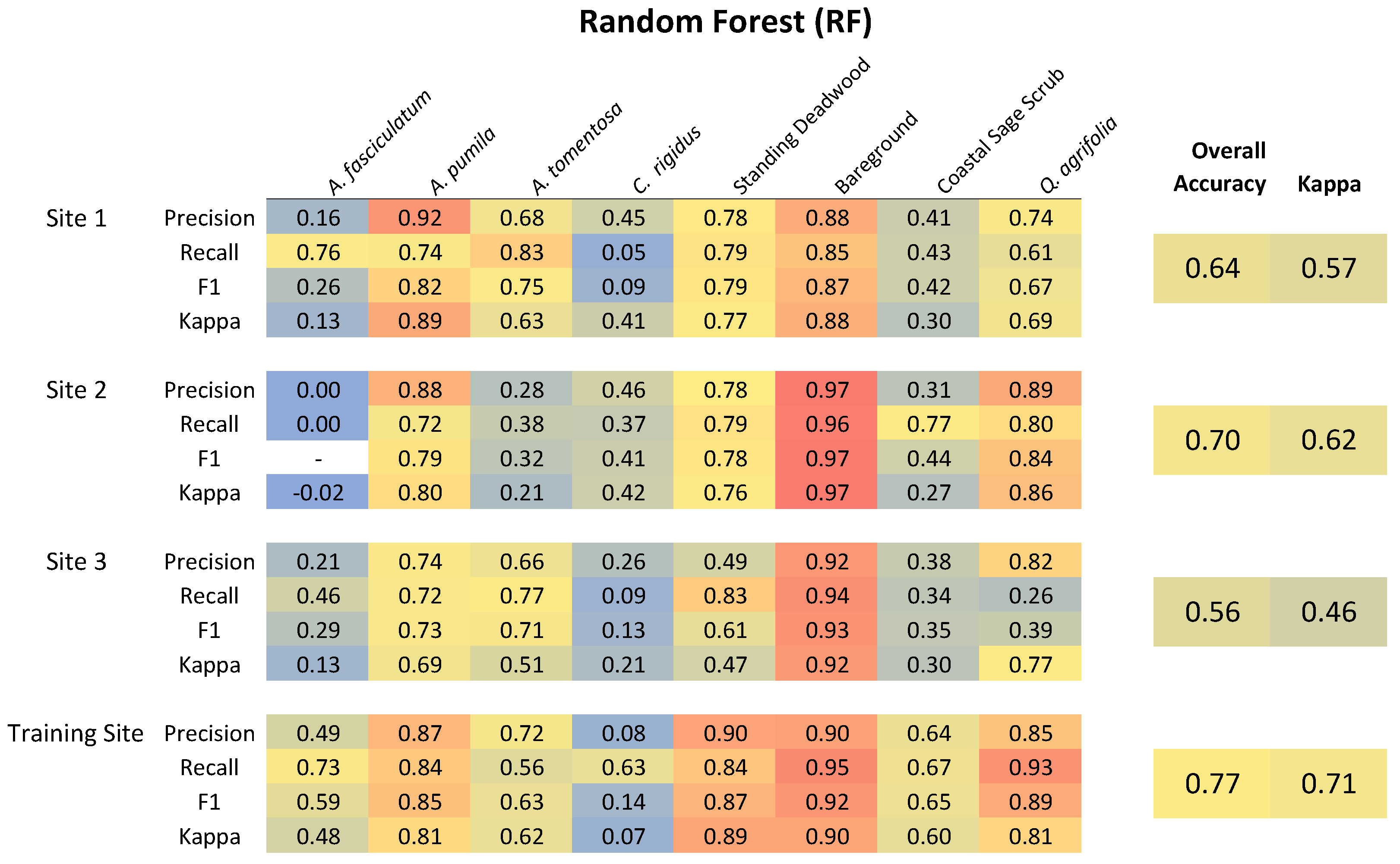
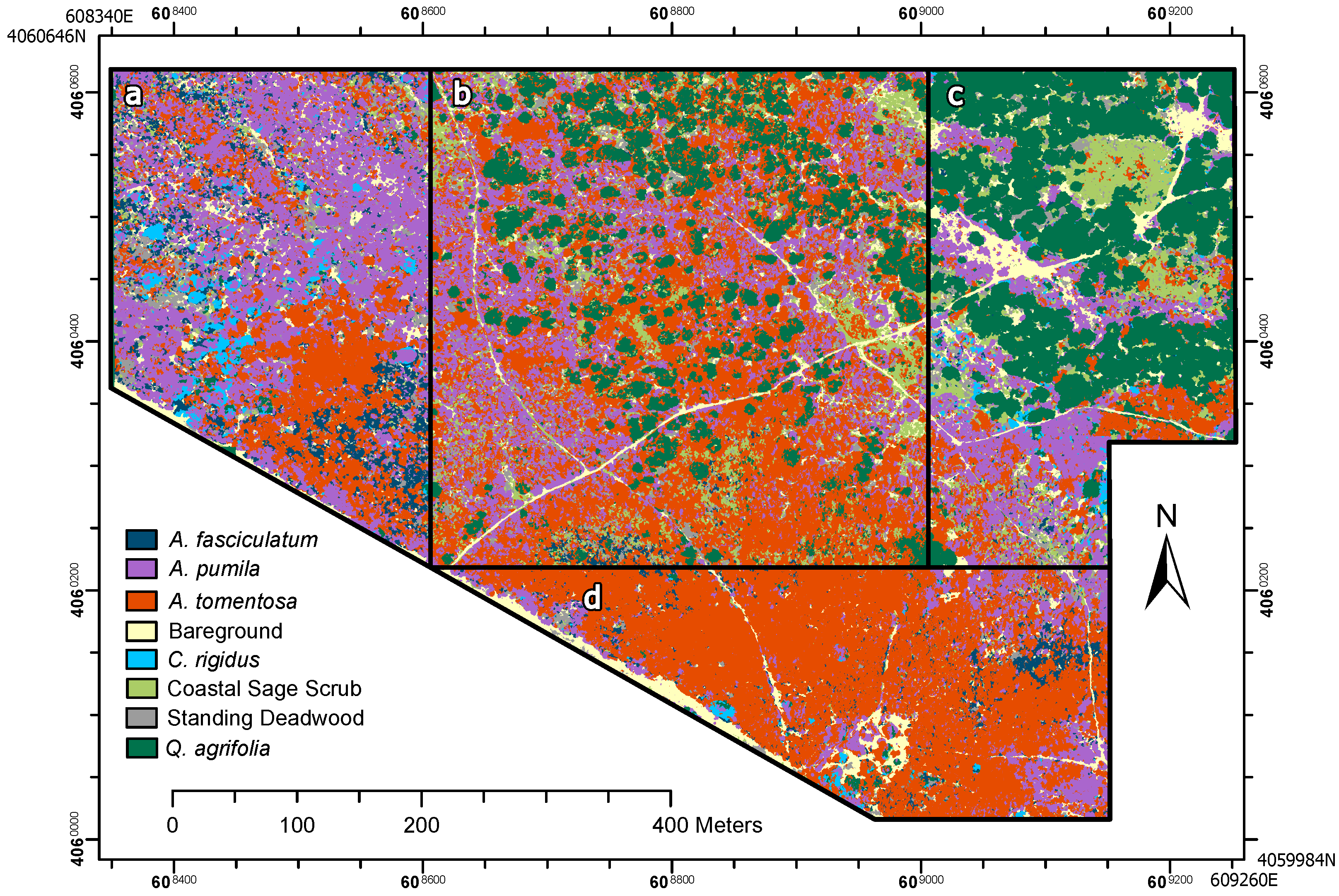
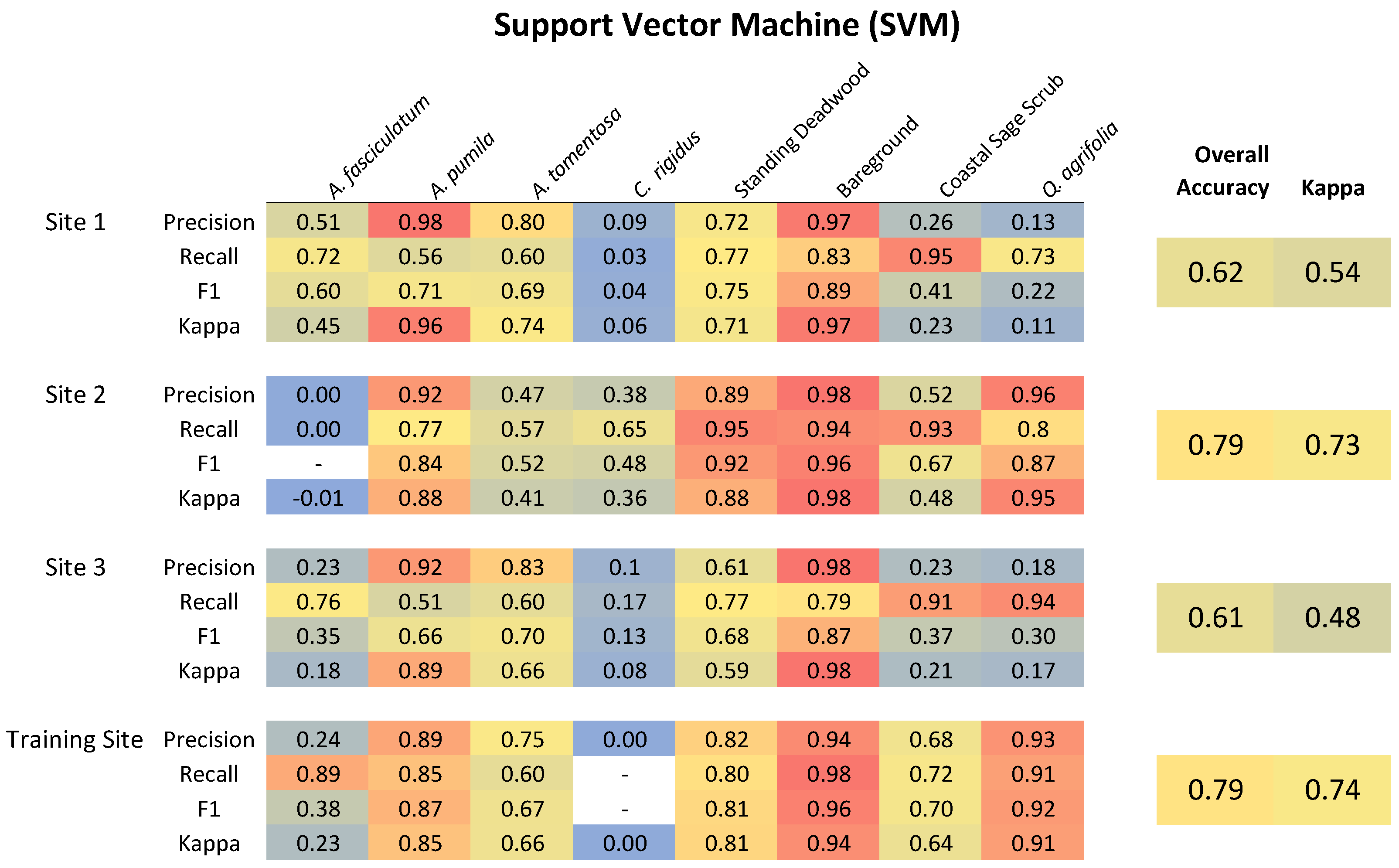
The classification performance of CNN + OBIA, RF, and SVM methods was assessed using visual inspection of classified segmentation polygons and quantitative accuracy assessment as object-based calculations of overall accuracy (OA) and Cohen’s Kappa coefficient ($\kappa$). In order to evaluate individual cover classes, we calculated per-class precision, recall, and F-Score (F1) statistics.

Precision [66], also called user accuracy, summarizes how often a real cover type on the ground (i.e., from reference data) correctly appears on the classified map. Recall, also called producer accuracy, describes how often the classes designated on the map are actually present on the ground.

A highly accurate classification must balance high recall and high precision. The F-Score (F1) statistic is a useful metric to evaluate the trade-off calculated as the harmonic mean of the precision and recall (Sundheim, 1992). A higher F1 statistic indicates support for predictions made by the model classifier. Another convention is to calculate Cohen’s kappa coefficient ($\kappa$), which compares observed patterns to a classification based entirely on random assignment. Kappa values range from −1 to 1; a value of 0 indicates that the classification is no better than random, and $\kappa$ close to 1 indicates that the classification is better than random.

3. Results

3.1. Field Survey Results

We collected a total of 11,622 ground survey points across the entire 40.7-ha research area (Table 2) The majority of data collection (60%) was concentrated within the 16-ha model training site, and the rest in the 24.7-ha application sites.

3.2. Classification Model Results

The CNN + OBIA method had the highest overall classification accuracy across all application sites ($MeanO{A}_{CNN+OBIA}=0.85, Mean{\kappa }_{CNN+OBIA}=0.81$) (Figure 7 and Figure 8) compared to random forest ($MeanO{A}_{RF}=0.63, Mean{\kappa }_{RF}=0.55$) (Figure A1 and Figure A2) and support vector machine ($MeanO{A}_{SVM}=0.67, Mean{\kappa }_{SVM}=0.58$) (Figure A3 and Figure A4). Our CNN + OBIA approach accurately classified three species of chaparral shrub species in the application sites including: A. fasciculatum ($Mean{\kappa }_{CNN+OBIA}=0.80$), A. pumila ($Mean{\kappa }_{CNN+OBIA}=0.86$), and A. tomentosa ($Mean{\kappa }_{CNN+OBIA}=0.72$). Random forest and SVM classification models were most effective at classifying A. pumila ($Mean{\kappa }_{RF}=0.79$, $Mean{\kappa }_{SVM}=0.91$), but only moderately accurate at classifying A. tomentosa ($Mean{\kappa }_{RF}=0.45$, $Mean{\kappa }_{SVM}=0.60$), and poor at classifying A. fasciculatum ($Mean{\kappa }_{RF}=0.08$, $Mean{\kappa }_{SVM}=0.21$). CNN + OBIA was the most effective model for classifying several other cover classes, including Q. agrifolia ($Mean{\kappa }_{CNN+OBIA}=0.97$), bareground ($Mean{\kappa }_{CNN+OBIA}=0.96$), standing deadwood ($Mean{\kappa }_{CNN+OBIA}=0.89$), and coastal sage scrub ($Mean{\kappa }_{CNN+OBIA}=0.69$). Rare Ceanothus rigidus classification accuracy was poor across all sites ($Mean{\kappa }_{CNN+OBIA}=0.28$, $Mean{\kappa }_{RF}=0.21$, $Mean{\kappa }_{SVM}=0.21$).

4. Discussion

Here, we presented a CNN + OBIA classification modeling approach based on very-high-resolution multispectral and structural UAV data capable of accurately identifying species, broader plant communities, and structural cover features in complex, wild vegetation. We attribute the success in our CNN + OBIA classification process to three factors: consideration of target species abundances and distribution across the training and application sites, collection of extensive ground survey training data, and integration of a CNN workflow that uses high resolution multispectral data with object-based segmentation based on multispectral and structural data. One distinct advantage of the CNN approach over RF and SVM is the ability to simultaneously classify a broad group consisting of several co-occurring species along with more focused and less variable target species. Our CNN + OBIA approach outperformed RF and SVM methods for classifying the heterogeneous coastal sage scrub group and several individual species.

We focused on creating an effective classification model for the four most dominant shrub and tree species in a dense and heterogeneous shrubland community; a reasonable next step would be to include additional species in the model. Generating a model is simple for locally dominant species because it is easiest to collect the needed training and testing data. Once a robust model is trained, it can be applied to other sites and evaluated with fewer survey points required for validation. Including less common species would require a larger suitable training area reflective of the composition of nearby application sites. The process of target species and training site selection are dependent on expert knowledge of regional plant communities. For example, the variable classification performance in A. fasciculatum in Site #2 (Figure A1) can be explained by the low abundance of A. fasciculatum. We were only able to locate nine distinct patches of A. fasiciculatum in Site #2 that met our ground survey criteria and six patches with neighboring coastal sage scrub, A. pumila, or C. rigidus causing a distinct drop in map reliability (recall) for this region. This means that care and creativity are needed when interpreting classification performance for locally rare species.

For example, the poor classification accuracy of Ceanothus rigidus provides a good example of what can happen when there are not an adequate number of specimens to adequately train the model and an inadequate number of validation points in application sites. In the case of C. rigidus the low number of available training subjects resulted in high recall rates, indicating that ground survey points were correctly identified in the map, but the low precision and accuracy statistics (F1, Kappa) indicating that the model misclassified other non-target points as C. rigidus. We were able to apply expert knowledge, and trial-and-error, to our classification fuzzy logic schema, setting a high probability threshold for classification of C. rigidus (p = 0.85) to reduce the prevalence of misclassification, although some misclassification persisted. This misclassification may be rectified by conducting lower elevation flights to gain higher resolution data, conducting surveys across much larger regions to increase the species sample abundance or by timing flights to coincide with the colorful seasonal bloom of C. rigidus.

Integrating structural features of the vegetation (i.e., canopy height and slope) with multispectral data into the multiresolution segmentation process was a powerful component in the identification of several species and structural features. For example, Quercus agrifolia was usually the tallest species in the landscape and had a consistently hemispherical crown shape that segmented well and helped produce a very high classification accuracy.

Grouping standing deadwood from multiple species into a single category may reduce the deadwood classification accuracy, as different species exhibit variations in dieback patterns and decay processes, which can be overlooked when combined. However, this aggregate approach can be effective at supporting the delineation of bareground, which often has similar spectral properties. In our study, manzanitas (A. pumila and A. tomentosa), chamise (A. fasciculatum), and oak (Q. agrifolia) were the predominant species exhibiting deadwood characteristics. In the future, creating separate classifications for each species could enhance classification accuracy and ecological relevance, providing a comprehensive understanding of dieback dynamics in the ecosystem. We attribute the high performance in deadwood detection to the abrupt variation in canopy heights and slope dynamics within manzanita and chamise dieback patches coupled with high NIR and NIR-edge absorption and low red absorption. Although our study does not delineate species-specific deadwood detection, it does offer a suitable alternative to rectifying a challenge with correctly classifying bareground from standing deadwood in forest systems [67].

We explored the use of a CNN + OBIA deep learning approach to classify vegetation cover at the species level using very high-resolution imagery collected using UAVs. Cover classification at these levels is essential for investigating the distribution and health of ecologically and economically important species in a variety of wildland, urban, and agricultural landscapes. This method holds great promise for supporting conservation management practices in wildland communities where target species may be located in inaccessible areas or distributed over large expanses, especially in heterogeneous wildland communities. The ability to accurately classify standing deadwood and areas of bareground is equally important as it could be used to study patterns of dieback and growth in these communities. A continuing challenge is the difficulty of collecting adequate data to train models for identification of locally rare species. Multiseasonal flights may capture phenological differences (i.e., flowering) useful for developing robust classification schema. The ease of flight planning and high-resolution sensor capabilities of drones make them well-suited for this type of research in the future.