Anomaly Detection for Data from Unmanned Systems via Improved Graph Neural Networks with Attention Mechanism

Abstract

Anomaly detection has an important impact on the development of unmanned aerial vehicles, and effective anomaly detection is fundamental to their utilization. Traditional anomaly detection discriminates anomalies for single-dimensional factors of sensing data, which often performs poorly in multidimensional data scenarios due to weak computational scalability and the problem of dimensional catastrophe, ignoring potential correlations between sensing data and some important information of certain characteristics. In order to capture the correlation of multidimensional sensing data and improve the accuracy of anomaly detection effectively, GTAF, an anomaly detection model for multivariate sequences based on an improved graph neural network with a transformer, a graph attention mechanism and a multi-channel fusion mechanism, is proposed in this paper. First, we added a multi-channel transformer structure for intrinsic pattern extraction of different data. Then, we combined the multi-channel transformer structure with GDN’s original graph attention network (GAT) to attain better capture of features of time series, better learning of dependencies between time series and hence prediction of future values of adjacent time series. Finally, we added a multi-channel data fusion module, which utilizes channel attention to integrate global information and upgrade anomaly detection accuracy. The results of experiments show that the average accuracies of GTAF, the anomaly detection model proposed in this paper, are 92.83% and 96.59% on two datasets from unmanned systems, respectively, which has higher accuracy and computational efficiency compared with other methods.

1. Introduction

Unmanned systems are characterized by low power consumption, flexibility and low cost, and can replace humans for difficult and intense tasks. In recent years, with the rapid development of unmanned systems, the safety of unmanned systems has attracted attention. Unmanned systems include unmanned systems platforms such as UAVs, unmanned ships and unmanned vehicles, among which UAVs are widely used and are the main research object of this paper. Detecting deviant data or behavioral patterns that do not match the expected behaviors from the normal data of UAVs and trying to find the reasons for the occurrence of abnormal behavior can prevent major accidents and guarantee the normal flight of UAVs, which is of great significance to improve the safety factor and the efficiency of the use of UAVs.

The study of anomaly detection for unmanned systems has attracted widespread attention. At present, anomaly detection methods are mainly divided into three categories: anomaly detection methods based on a priori knowledge, model-based anomaly detection methods and data-driven anomaly detection methods.

A priori knowledge-based is one of the earliest anomaly detection algorithms that synthesizes data from the UAV target system and builds an anomaly detection model applicable offline based on the expert’s prior knowledge. For example, Sun et al. [1] built a system knowledge base for UAVs based on a hierarchical fault cause structure map. Liu et al. [2] studied the UAV flight control system based on the fault tree analysis method and transformed the expert experience into a fault knowledge base based on the correspondence between the sign space and the fault space. Singh et al. [3] proposed an expert system integrating knowledge-based and model neural networks. Qing et al. [4] established an aircraft fault diagnosis expert system based on case-based reasoning, using a combination of hierarchical retrieval and nearest neighbor algorithm. However, anomalies in UAVs are sometimes difficult to grasp, the a priori knowledge-based approach requires accurate and complete expert knowledge, and the manual knowledge acquisition and model construction process is time-consuming and labor-intensive.

The model-based anomaly detection method requires the establishment of an accurate physical model to describe the operating characteristics of the UAV for the purpose of identifying anomalous data. For example, Chen et al. [5] used FLUENT and ANSYS software for finite element simulation analysis to determine the fault monitoring nodes, and finally used the beacon anomaly analysis method to detect anomalies in the data. Tan et al. [6] introduced a model correction link to reduce the long-term cumulative error of the system in dynamic operation. Melnyk et al. [7] constructed a distance matrix between objects based on a vector autoregressive exogenous model between objects and finally performed anomaly detection based on object differences. Liu et al. [8] studied a fault detection algorithm for a UAV control system based on parameter estimation, using the noise estimator to diagnose the fault, and analyzed the relationship between the residual and “zero” so as to realize the fault detection. Yang et al. [9] proposed a dynamic data fusion model, which fuses and predicts the physical parameters of the turbofan engine. However, the portability of the established model is poor, and each UAV system needs to be modelled separately, which is not practical.

Data-driven anomaly detection methods based on data do not require accurate mechanistic rules and complete expert knowledge, and are performed by analyzing the correlation of UAV sensor data and building an effective anomaly detection model. For example, Bronz et al. [10] classified the behavior of the UAV in the normal flight phase and the fault phase based on the SVM algorithm. Yaman et al. [11] used the SVM algorithm to classify audio signals and designed a lightweight fault detection algorithm. Pan [12] established a parameter prediction model based on the genetic algorithm to improve and optimize the neural network. Lv et al. [13] designed a combination of Bayesian information criterion-based density peak clustering analysis algorithm and shared neighborhood algorithm to accurately classify and label aeroengine data. Pan et al. [14] introduced a modified S3VM combined with edge sampling to actively learn an optimized classification model for anomaly detection on UAV channel telemetry data. Ahmad et al. [15] compared the UAV data anomaly detection algorithm based on multiple LSTM and multi-output convolution LSTM, and pointed out that multi-output convolution LSTM is more suitable for multi-dimensional time data analysis of UAVs. You et al. [16] proposed an algorithm based on Time Convolutional Network (TCN) model delivery for a UAV sensor data anomaly detection method, which uses a threshold detection method to determine whether there are anomalies in the UAV sensor data. Li et al. [17] used the LSTM neural network to make a difference between the predicted value and the real value, and judged whether the data are abnormal or not by the distance from the test data to the hyperplane. In order to make the relevant research a more intuitive presentation [18,19,20,21], we list it in the form of a table, as shown in

Table 1. Comparative analysis of state-of-the-art surveys.

Research	Year	Objective	Dataset	Accuracy	Limitations
Bronz et al. [10]	2020	The SVM algorithm of the characteristic trajectory	Flight Log	95%	The computational limitations of the inference hardware should be carefully taken into account during training
Yaman et al. [11]	2022	A lightweight method has been proposed for the early detection of faults in UAV motors	Helicopter;	100%;	Fault settings are not comprehensive
			Duocopter;	100%
			Tricopter;	99.06%;
			Quadcopter	90.53%
Pan et al. [12]	2021	Established ANN-NARX parameter prediction model for aeroengine	Actual flight test data of an engine sortie	95.2%	Fault simulation state recognition rate is relatively low
Lv et al. [13]	2020	DPCA algorithm based on unsupervised learning	Aeroengine gas path component fault data	91%	Experimental analysis with simulated data
Pan et al. [14]	2020	An anomaly detection model based on active learning and improved S3VM classification	Telemetry data from UAV	Labeled samples 5: 90.8%;	Labeled sample classification is less
				Labeled samples 10: 92.7%
Ahmad et al. [15]	2022	Compared two deep learning tools to detect anomalies in the values of the UAV attributes	Data from four flights of a fixed-wing aircraft called Thor	Average: 90%	Less precision when detecting anomalies in consecutive faults
You et al. [16]	2022	An FTCN-based Anomaly Detection Framework	The flight data of the UAV in a calm environment and in a crosswind environment of 3 m/s	94.76%	Fine-tuning the model on a small training dataset in the source domain leads to biased predictions
Li et al. [17]	2021	Prediction and Anomaly Detection Using LSTM Neural Networks	GPS and IMU sensor data, ground street view image data	Average: 90.68%	The detection rate of random position offset attack and replay attack is not high enough

.

The Graph Deviation Network (GDN) model [22] is a multivariate time series anomaly detection method based on graph neural networks, which performs anomaly determination by learning a graph of relationships between data patterns and obtaining anomaly scores through prediction and deviation scoring based on an attention mechanism. However, in complex multi-dimensional time series problems, GDN has shortcomings in two aspects. Firstly, the GAT module is susceptible to over-smoothing as the GAT module may suffer from over smoothing when the graph data are very dense and have highly correlated characteristics, leading to loss of information and not capturing local features of the data and global features of the data well [23,24]. Secondly, GDN does not fully utilize edge features, as GDN exploits connectivity only, resulting in a failure to properly merge feature patterns from different data [25]. These two aspects make the accuracies of prediction and anomaly detection using GDN relatively low in multidimensional time series problems.

In view of the above two problems, the GDN model is improved, and an anomaly detection model, GTAF (an improved GDN model with transformer [26], graph attention network [27] and multi-channel fusion mechanism), is proposed in this paper for the anomaly detection of sensing data from unmanned systems. GTAF adopted GDN as the base framework and added a multi-channel transformer model for the prediction and a multi-channel data fusion module for the prediction results fusion. In GTAF, the multi-channel transformer model is combined with the original graph attention network (GAT) of GDN to capture the features of time series and learn the dependencies between them better so as to predict future values of adjacent time series more accurately; the multi-channel data fusion module is added to optimize the prediction of time series and improve the anomaly detection accuracy.

The primary contributions of this paper are as follows: (1) We proposed a new anomaly detection model, GTAF, which adds a multi-channel transformer and combines it with GAT to successfully enhance the prediction capacity. (2) We added a multi-channel data fusion module to aggregate the results of different channels and integrate information to obtain better prediction results, further enhance the abnormal score, and attain good detection performance. (3) Extensive experiments were conducted by comparing the performance of GTAF with other models (such as iForest [28], LOF [29], DAGMM [30], and OmniAnomaly [31], etc.), as well as ablation experiments, in order to verify the performance of GTAF.

The remaining parts of this paper are organized as follows. Section 2 introduces the materials and methods: Section 2.1 describes the framework of GNN, Section 2.2 defines the problem, Section 2.3 details the main idea of the GTAF model and the basic principles involved, Section 2.4 explains the dataset of this paper and Section 2.5 elaborates experimental design. Section 3 introduces the experimental results and discussion: Section 3.1 describes the attribute correlation experiment of the GFTD dataset, Section 3.2 describes the comparison experiment of anomaly detection, Section 3.3 is the evaluation for anomaly types, Section 3.4 describes the ablation experiments and Section 3.5 describes a parameter sensitivity experiment. Finally, Section 4 presents the conclusion of the work.

2. Materials and Methods

2.1. Problem Definition

In order to detect the anomalies in sensing data from unmanned systems, anomaly detection methods based on prediction for multidimensional time series predict the value using a pre-trained model and then use the distance between the true value and the predicted value as the anomaly score. The following symbols are defined in the model:

• Dt: Time series data as input.
• $i$: Index of nodes in the graph for the sensing data time series.
• $v_i$: Similarity of the multivariate time series, $v_i\in R^d$, $i\in \left\{1,2,\dots ,N\right\}$, and $d$ denotes the number of nodes in the graph.
• $A_{ij}$: Relationship between nodes, representing the edge from node $i$ to node $j$, i.e., the directed relation between node $i$ and node $j$.
• $e_{ji}$: Similarity between the embedding vector $v_i$ and its candidate relation $C_i$.
• $U_i^{time}$: Input value with time information.
• $U_i^{norm}$: Normalized value of time information.
• $C_i^{en}$: Final hidden vector matrix encoded.
• $H_i^s$: Prediction result by multichannel attention after linear transformation.
• ${\tilde{Y}}_t^s$: Prediction result after multi-channel data fusion.
• $Er{r}_i\left(t\right)$: Deviation between predicted and measured values.
• $a_i\left(t\right)$: Deviation after normalization.
• $A\left(t\right)$: Exception score after aggregation of the function.
• $A_s\left(t\right)$: Exception score after simple moving average (SMA) processing.

The problem to be solved for GTAF, the anomaly detection model proposed in this paper, is to take the sensing time series Dt as input and obtain the corresponding anomaly detection evaluation score $A_s\left(t\right)$ so as to determine the anomaly detection result based on the relationship between the score and the threshold value.

2.2. The Framework of GNN

The purpose of GNN is to learn a state embedding vector, $h_v\in R^s$, for each node, which contains the information of each node’s neighbor nodes. $h_v$ represents the state vector of the node; this vector can be used to generate the output $o_v$. Assume that $f\left(\cdot \right)$ is a function with parameters, called a local transition function; this function is shared among all nodes and updates the node state according to the input of neighboring nodes. Suppose $g\left(\cdot \right)$ is a local output function (local output function), which is used to describe how the output is generated:

$$h_v=f\left(x_v,x_{co\left[v\right]},h_{ne\left[v\right]},x_{ne\left[v\right]}\right)$$

(1)

$$o_v=g\left(h_v,x_v\right)$$

(2)

$x_{co\left[v\right]}$ represents the feature vector of node v, $h_{ne\left[v\right]}$ represents the feature vector of the edge associated with node v, $x_{ne\left[v\right]}$ represents the state vector of the neighbor node of node v, and $x_{ne\left[v\right]}$ represents the feature vector of the neighbor node of node v. Assuming that all the state vectors, all output vectors, all feature vectors and all node features are superimposed and represented by $H$, $O$, $X$, $X_N$, respectively, then a more compact representation can be obtained:

$$H=F\left(H,X\right)$$

(3)

$$O=G\left(H,X_N\right)$$

(4)

Among them, F and G are respectively called the global transfer function and the global output function, which are the stacked versions of $f$ and $g$ for all nodes in the graph. According to Banach’s fixed point theorem, GNN uses the following traditional iterative method to calculate the state parameters:

$$H^{t+1}=F\left(H^t,X\right)$$

(5)

Among them, $H^t$ represents the tensor of the iterative cycle of $t$. For any initial value $H_0$, Equation (5) can quickly converge to obtain the final fixed-point solution of Equation (3).

2.3. GTAF Model

2.3.1. Main Idea

The GTAF model proposed in this paper is an anomaly detection method for time series data based on graph neural networks, and its structure is shown in Figure 1.

As can be seen from Figure 1, the GTAF model mainly includes four steps, which are listed as follows:

(1)

Relevance learning: According to the sensing data inputted, graph nodes embedding vectors are set up, and then the directed graph is constructed so as to associate the features in sensing data and facilitate information exchange. After that, the similarity between vectors embedded in the nodes and their candidate relationships are calculated.

(2)

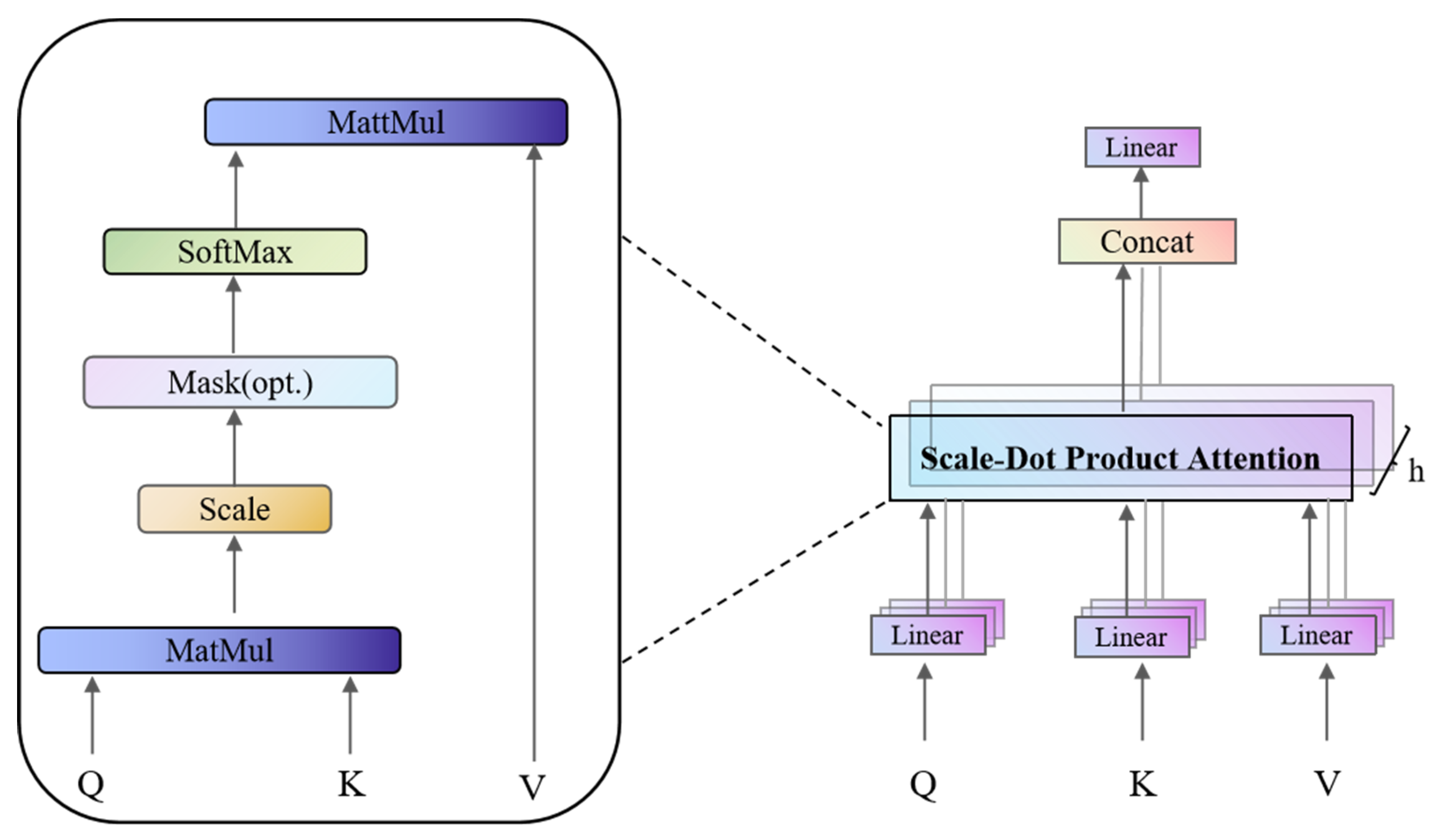
Prediction with Transformer and GAT: The sensing data contextual information vectors are obtained using Transformer. The temporal information is processed and fed into the multi-headed attention mechanism, and then layer normalization is performed to prevent gradient disappearance or gradient explosion. The interdependencies between the multivariate sequences are captured using the graph attention network (GAT), and finally the prediction results are obtained.

(3)

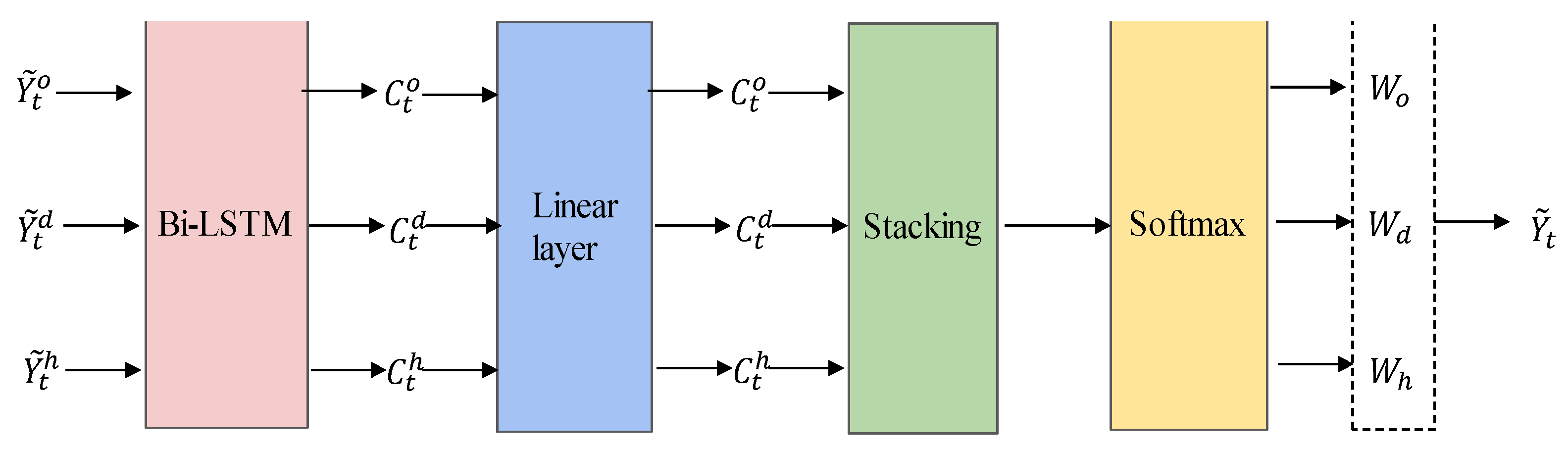
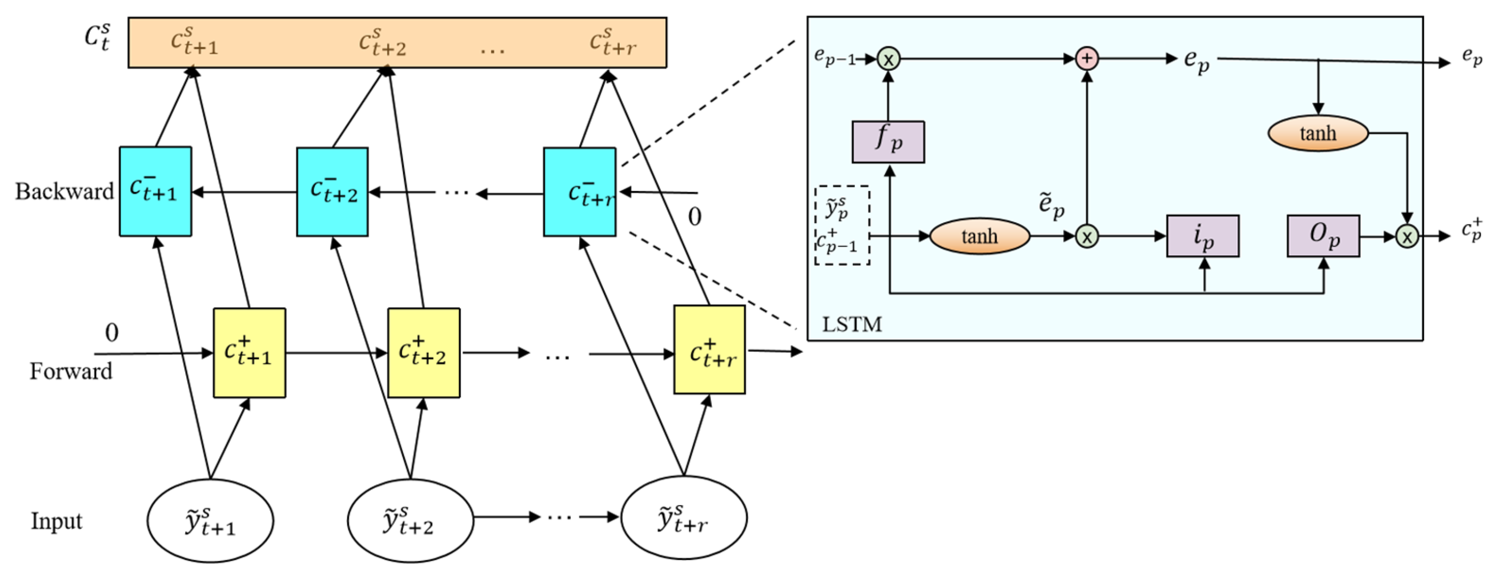
Multi-channel data fusion: Based on the multi-channel transformer mechanism, the characteristics of different sensing data are integrated using the bi-directional long short-term memory network (Bi-LSTM) [32] as the structure for computing channel attention, and then the results of different channels are evaluated and aggregated according to the evaluation weights; the mean square error is used as the loss function.

(4)

Anomaly judgement: The deviation between the predicted value and the observed value is calculated, normalized and then aggregated using an aggregative function to obtain the score for the final anomaly judgement.

2.3.2. Relevance Learning

In the proposed model, GTAF, graph structure is used to learn the dependencies among sensing data. In many multivariate time-series data, each of the time series may possess features highly deviating from others, and these features can be associated with each other in very complex ways. Relevance learning means to capture the relevance among different features of their behaviors in a multi-dimensional way.

(1)

Vector definition

A vector $v_i$ is defined to represent the similarity of the multivariate time series, where $v_i\in R^d$, $i\in \left\{1,2,\dots ,N\right\}$, $i$ denotes the time series nodes and $d$ denotes the number of nodes.

(2)

Establishment of directed graph

A directed graph is constructed according to the relationships between multivariate time series data, in which nodes represent data of the time series and the edges represent the feature relationships among the nodes, and the adjacency matrix of the directed graph is denoted as $A$.

(3)

Similarity calculation

For each node $i$, its dependency candidate relation is expressed as $C_i\in \left\{1\dots \dots ,N\right\}/\left\{i\right\}$. If a priori information is available, $C_i$ can be customized; otherwise, it is the full set except itself. For node $i$, the similarity $e_{ji}$ of the embedding vector of node $i$ to its candidate relation $C_i$ can be calculated using Equation (6):

$$e_{ji}=\frac{v_i{}^T{v}_j}{\Vert v_i\Vert ·\Vert v_j\Vert }, for j\in C_i$$

(6)

The first $k$ such normalized dot product is then selected, and TopK means the normalized metric for the first $k$ values. The elements $A_{ji}$ in the directed graph $A$ can be expressed as Equation (7). The value of $k$ can be determined according to the desired sparsity:

$$A_{ji}=1, \left\{j\in TopK\left(\left\{e_{ki}:k\in C_i\right\}\right)\right\}$$

(7)

2.3.3. Prediction with Transformer and GAT

In the proposed GTAF model, the multi-channel transformer mechanism and graph attention network (GAT) are integrated to optimize the prediction performance. The transformer is used to obtain the contextual information vector and the GAT is used to capture the interdependencies between user behaviors in order to achieve better prediction results of the model.

(1)

Embedding temporal information

The biggest feature of the transformer model is that it discards network structures such as RNNs and CNNs. The transformer model initially showed its talents in the field of machine translation. In recent years, many scholars have applied it to the fields of sequence data prediction and target detection, and have achieved good results [33]. Guo et al. [34] constructed an attention-based spatio-temporal graph network model for the prediction of traffic flow, where the attention was implemented using the transformer model. Xu et al. [35] built a spatio-temporal feature extraction module using the encoding block of the transformer.

The structure of a single channel transformer is shown in Figure 2. In GTAF, a three-channel transformer structure is used. The inputs to the transformer in the different channels are expressed as $X_i^s$, $\left(s=o,d,h\right)$. For the encoding layer, since the dimension size of the input is not the same as that of the output, it is necessary to embed the input matrix $O_i$ into the hidden layer dimension space to facilitate the correlation operation with the decoding layer. The calculation is as Equation (8):

$$E_i^{emb}=X_i^s{W}_s^{en}+b_s^{en}$$

(8)

In Equation (8),$W^{en}\in R^{n\times d_{\mathrm{model}}^s}$, $d_{\mathrm{model}}^s$ indicates the size of the hidden layer of the Transformer structure for that channel.

In GTAF, considering that the Transformer structure does not carry sequential information, temporal information is added to the model in order to fully exploit the temporal properties of the multivariate time series data.

The temporal labels are discretized using one-hot encoding, then all the codes are stitched together. Suppose that the stitched vector is $T_i^{en}\in R^{l\times d_{time}}$, where $d_{time}$ denotes the length of the stitched codes. Then a mapping matrix is generated according to Equation (9) to map $T_i^{en}$ to the dimension of the coding structure:

$$PE\left(pos,L\right)=\left\{\begin{array}{c}sin\left(pos/{\text{10,000}}^{\frac{l}{d_{\mathrm{model}}^o}}\right),i \mathrm{is} \mathrm{even} \mathrm{number}\\ cos\left(pos/{\text{10,000}}^{\frac{l}{d_{\mathrm{model}}^o}}\right),i \mathrm{is} \mathrm{odd} \mathrm{number}\end{array}\right.$$

(9)

In Equation (9), $pos\in \left[1,d_{time}\right]$ indicates the position of $T_i^{en}$ in the sequence, and $l\in \left[1,d_{\mathrm{model}}^s\right]$ indicates the dimension to be mapped. Using the above equations, the dimensional transformation matrix can be expressed as $A_s^{en}\in R^{d_{time}\times d_{\mathrm{model}}}$. As a result, the input with temporal information can be calculated using Equation (10), where $d_{label}$ means the number of time labels:

$$U_i^{time}=\frac{T_i^{en}{A}_s^{en}}{\sqrt{d_{label}}}+U_i^{emb}$$

(10)

Next, the temporal information $U_i^{time}$ is fed into the multi-headed attention module to adjust the sequence characteristics, as is shown in Figure 3, where the inputs $Q,K,V$ are all $U_i^{time}$. The calculation in Figure 3 can be expressed as Equation (11):

$$\begin{array}{r}\mathrm{MultiHead}\left(Q,K,V\right)=\mathrm{Concat}\left({\mathrm{head}}_1,\dots {,\mathrm{head}}_h\right)W_s^{en}\\ {\mathrm{head}}_l=\mathrm{Attention}\left(Q{W}_{Q,l}^{en},K{W}_{V,l}^{en},V{W}_{V,l}^{en}\right)=\\ \mathrm{Softmax}\left(\frac{Q{W}_{Q,l}^{en}{\left(K{W}_{K,l}^{en}\right)}^T}{\sqrt{d_k}}\right)V{W}_{V,l}^{en}\end{array}$$

(11)

In Equation (11), $W_s^{en}\in R^{h{d}_v\times d_{\mathrm{model}}^s}$, $W_{Q,l}^{en}\in R^{d_{\mathrm{model}}^s\times d_k}$,$W_{K,l}^{en}\in R^{d_{\mathrm{model}}^s\times d_k}$, $W_{V,l}^{en}\in R^{d_{\mathrm{model}}^s\times d_v}$, where $h$ denotes the number of attention heads, $d_k=d_v=d_{\mathrm{model}}^s/h$ and $T$ means the transpose operation of a matrix.

(2)

Layer normalization

Suppose the result matrix is $U_i^{self}$ after completing the adjustment. Considering that some information may be lost during the adjustment, the original input is added to the result matrix according to the idea of residual networks, so as to keep the completeness of all information. The calculation is as Equation (12):

$$U_i^{norm}=\mathrm{LN}\left(U_i^{self}+U_i^{time}\right)$$

(12)

In Equation (12), $\mathrm{LN}$ denotes the layer normalization method [36]. The purpose of layer normalization is to effectively prevent gradient disappearance or gradient explosion.

(3)

Dependency capture

In GTAF, a graph attention network is used to capture the interdependencies among data. Suppose that the graph contains N nodes, each with a feature vector of $G_i$ and dimension $F$, as Equation (13) shows:

$$G=\left\{G_1,G_2,\dots ,G_N\right\}$$

(13)

A new feature vector ${\delta }_i^{\prime }$ can be obtained after performing a linear transformation to the node feature vector $G$, as Equations (14) and (15) show:

$${\delta }^{\prime }=W{G}_i$$

(14)

$${\delta }^{\prime }=\left\{{\delta }_1^{\prime },\dots \dots ,{\delta }_N^{\prime }\right\}$$

(15)

In Equation (14), $W\in R^{F^{\prime }\times F}$ is the matrix of the linear transformation, where $F^{\prime }$ is the dimension of the transformation matrix.

The feature vectors of the node $i$ and node $j$ are stitched together, and then the inner product is calculated with a $2F^{\prime }$ dimensional vector $a$. The LeakyRelu function is adopted as the activation function, as is shown in Equations (16) and (17):

$$a_{ij}=\frac{exp\left(\mathrm{LeakyRelu}\left(a^T\left[W_s{\delta }_i^{\prime }\Vert W_s{\delta }_j^{\prime }\right]\right)\right)}{{{\displaystyle \sum }}_{k\in N_i}exp\left(\mathrm{LeakyRelu}\left(a^T\left[W_s{\delta }_i^{\prime }\Vert W_s{\delta }_j^{\prime }\right]\right)\right)}$$

(16)

$${\tilde{G}}_i^{\prime }=\mathrm{concat}\left(\sigma \left({\displaystyle \sum }_{j\in N_i}{a}_{ij}^k{W}_s{}^k{\tau }_j\right)\right)$$

(17)

At the end of the coding layer, the final encoded hidden vector matrix is obtained by a simple feed-forward network with a non-linear mapping and a combination with the residual. The equation is as Equation (18), where $W_{s,0}^{en}\in R^{d_{\mathrm{model}}^s\times 2d_{\mathrm{model}}^s}$, $W_{s,1}^{en}\in R^{2d_{\mathrm{model}}^s\times d_{\mathrm{model}}^s}$.

$$C_i^{en}=\mathrm{LN}\left(U_i^{norm}+\mathrm{Relu}\left(U_i^{norm}{W}_{s,0}^{en}+b_{s,0}^{en}\right)W_{s,1}^{en}{\tilde{G}}_i^{\prime }+b_{s,1}^{en}\right)$$

(18)

(4)

Decoding

The input for the part of the decoding layer is unknown, so an initial value is needed to start decoding. The output value $y_i$ is used as the initial activation value, and other positions are all set to 0 for the beginning. Suppose the input matrix is ${\tilde{Y}}_i^{s,temp}$ and the result after time encoding is ${\tilde{Y}}_i^{s,time}$. The attention module in the decoder is different from that in the encoder. Because the future cannot be seen in the decoder, a mask is added to hide the data of the future, and then the output is obtained after connecting the residuals using layer normalization.

In the core of the decoder, the multi-headed attention modules $Q,K,V$ are ${\tilde{Y}}_i^{s,norm}$, $C_i^{en}$ and $C_i^{en}$, respectively, where ${\widetilde{ Y}}_i^{s,norm}\in R^{1\times d_{\mathrm{model}}^s}$ represents the data of the last valid time slot, through which the impact of different past time slots on the future can be captured flexibly. Suppose the current valid time slot is $t$; the decoder hidden vector $c_{t+1}^{de}$ can be obtained through a simple feed-forward network with residual connections, and finally the predicted output of $t+1$ is obtained through a linear mapping. The calculation is as Equation (19):

$${\tilde{y}}_{t+1}^s=c_{t+1}^{de}{W}_s^{de}+b_s^{de}$$

(19)

In Equation (19), $W_s^{de}\in R^{d_{\mathrm{model}}^s\times m}$. After replacing ${\tilde{y}}_{t+1}^s$ with the data from the $t+1$ time slot in ${\tilde{Y}}_t^{s,temp}$, the decoding continues to the next step, where the last valid time slot becomes $t+1$. The final prediction for the channel ${\tilde{Y}}_t^s$ is obtained after r cycles.

2.3.4. Multi-Channel Data Fusion

Predicted values can be obtained using a single-channel transformer mechanism, but it also has some limitations. Therefore, in GTAF, a multi-channel transformer mechanism is used to make full use of the characteristics of each channel. The results of different channels using the channel attention approach are evaluated and aggregated according to the evaluation weights so as to obtain a better prediction performance. The overall process is shown in Figure 4.

(1)

Evaluation of channel attentions

In GTAF, the bi-directional long short-term memory (Bi-LSTM) network is used as the base structure for the calculation of channel attentions, as is shown in Figure 5.

Suppose the predicted values obtained for the three channels are ${\tilde{Y}}_i^o$, ${\tilde{Y}}_i^d$, and ${\tilde{Y}}_i^h$, respectively. For the predicted value of a channel time slot:

$$c_p^s=\mathrm{Concat}\left({\mathrm{LSTM}}^{+}\left({\tilde{y}}_p^s,c_{p-1}^{+};{\lambda }^{+}\right), {\mathrm{LSTM}}^{-}\left({\tilde{y}}_p^s,c_{p+1}^{-};{\lambda }^{-}\right)\right)$$

(20)

In Equation (20), ${\mathrm{LSTM}}^{+}$ and ${\mathrm{LSTM}}^{-}$ denote the forward and reverse LSTM cells, respectively; ${\lambda }^{+}$ and ${\lambda }^{-}$ denote their parameters, respectively; $c_{p-1}^{+}$ and $c_{p+1}^{-}$ denote the previous output states of ${\mathrm{LSTM}}^{+}$ and ${\mathrm{LSTM}}^{-}$ at the time of inputting, respectively. The size of $c_p^s$ is $2d_{\mathrm{fusion}}$, and $d_{\mathrm{fusion}}$ is the size of the hidden vector of the forward or inverse LSTM. The calculations inside the forward and reverse LSTM cells are shown as Equations (21)–(26):

$$f_p=sigmoid\left(W_1\left[{\tilde{y}}_p^s,c_{p-1}^{+}\right]+b_1\right)$$

(21)

$$i_p=sigmoid\left(W_2\left[{\tilde{y}}_p^s,c_{p-1}^{+}\right]+b_2\right)$$

(22)

$$o_p=sigmoid\left(W_3\left[{\tilde{y}}_p^s,c_{p-1}^{+}\right]+b_3\right)$$

(23)

$${\tilde{e}}_p=tamh\left(W_4\left[{\tilde{y}}_p^s,c_{p-1}^{+}\right]+b_4\right)$$

(24)

$$e_p=f_p\odot e_{p-1}+i_p\odot {\tilde{e}}_p$$

(25)

$$c_p^{+}=o_p\odot tanh\left(e_p\right)$$

(26)

In the above equations, $f_p$, $i_p$ and $o_p$ represent the results of the forgetting, input and output gates, respectively, at the time slot, and $e_p$ is the state inside the LSTM cell.

(2)

Aggregation

First, a linear transformation is performed, which can be achieved by Equation (27), where $W_L\in R^{2d_{\mathrm{fusion}}\times m}$.

$$H_i^s=C_i^s{W}_L,\left(s=o,d,h\right)$$

(27)

Next, it is stacked to obtain $H_i\in R^{r\times m\times 3}$, then the Softmax function is executed on the last dimension of $H_i$, and the last dimension of its result is split into three parts to obtain $W_o$, $W_d$, and $W_h$.

The final prediction can be achieved by aggregation according to Equation (28):

$${\tilde{Y}}_i=W_o\odot {\tilde{Y}}_i^o+W_d\odot {\tilde{Y}}_i^d+W_h\odot {\tilde{Y}}_i^h$$

(28)

(3)

Error minimization

The predicted output of the model should be as close as possible to the true value, so the mean square error between the predicted output ${\tilde{Y}}_i{}^{\left(t\right)}$ and the observed data $Y_i{}^{\left(t\right)}$ is used as a loss function to minimize the error.

$$L_{MSE}=\frac{1}{T_{train-w}}{{\displaystyle \sum }_{t=w+1}^{T_{train}}\Vert {{\tilde{Y}}_i}^{\left(t\right)}-Y_i{}^{\left(t\right)}\Vert }_2^2$$

(29)

2.3.5. Anomaly Judgement

To detect anomalies, the deviation between the predicted and observed values of node $i$ at time $t$ can be calculated as Equation (30):

$$Er{r}_i\left(t\right)=\left|Y_i^{\left(t\right)}-{{\tilde{Y}}_i}^{\left(t\right)}\right|$$

(30)

Then the deviation of each data item is normalized according to Equation (31), where ${\tilde{\mu }}_i$ is the median of $Er{r}_i\left(t\right)$ and ${\tilde{\sigma }}_i$ is the interquartile range of $Er{r}_i\left(t\right)$:

$$a_i\left(t\right)=\frac{Er{r}_i\left(t\right)-{\tilde{\mu }}_i}{{\tilde{\sigma }}_i}$$

(31)

To express the result of anomaly detection of data item at the time $t$, the function $max$ is used for aggregation.

$$A\left(t\right)=\underset{i}{max}{a}_i\left(t\right)$$

(32)

Finally, simple moving average (SMA) is used to generate a smoothing score $A_s\left(t\right)$. If the value of $A_s\left(t\right)$ exceeds a preset threshold, the data item at the time slot $t$ is marked as an anomaly.

2.4. Datasets

The purpose of this paper is to use the GTAF model to detect anomalies in unmanned system data. The following two data sets were chosen as the experimental data for the experiments in this paper.

(1)

GFTD [37]

The dataset contains data of antenna components from 1 January 2016 to 31 December 2016, including 8 remote sensing attributes: antenna temperature, current, switch status information, etc., and 2 status attributes: working or emergency stop, as shown in

Table 2. Attributes in the dataset GFTD.

Components	Attribute Code	Attribute Description
Azimuth axis	TB8	Temperature
	IB1	Current
Elevation axis	TB3	Temperature
	IB2	Current
Cable	TB9	Cable temperature
Signal antenna	TB2	Temperature
	VB11	Power status
	ZL5	Heater
	ZB1_EMG	Emergency stop status #1
	ZB2_EMG	Emergency stop status #2

.

The anomalies of the GFTD dataset are classified into three types: point anomalies, collective anomalies and correlation anomalies [38]. A point anomaly means an outlier in a set of data points. A collective anomaly refers to the fact that an individual may not be anomalous when checked individually, but the simultaneous occurrence of these individuals forms an anomaly. An association relationship anomaly means that there are correlations among the data and an anomaly exists for the correlations. The three types of anomalies in the dataset GFTD are described in detail in

Table 3. Description of GFTD dataset anomalies.

ID	Anomaly Type	Amount
1	Point anomalies	60
2	Collective anomalies	80
3	Association anomalies	242

.

(2)

SMAP [39]

This dataset SMAP (Soil Moisture Active Passive) contains a total of 429,735 data items from 55 remote sensing channels, including 24 categories, and is divided into four levels: L1, L2, L3 and L4. The L1 attributes contain instrument-related data and are presented as granules based on SMAP half-orbits. The L2 attributes are geophysical soil moisture data on fixed Earth grids based on L1 attributes and auxiliary information. The L3 attributes are daily complex data based on L2 attributes and freeze-thaw status data. The L4 attributes provide global spatial and temporal information on permafrost and soil moisture, which are model-derived value-added data attributes for soil moisture and net ecosystem exchange of carbon at the surface and root zone. The details of the dataset SMAP are shown in

Table 4. Details of the SMAP dataset.

Attribute Code	Attribute Description	Gridding (Resolution)
L1A_Radiometer	Parsed radiometer remote sensing	-
L1A_Raddar	Parsed SMAP radar remote sensing	-
L1B_TB	Geolocated, calibrated brightness temperature in time order	36 km
L1B_TB_E	Backus-Gilbert interpolated, calibrated brightness temperature in time order	9 km
L1B_S0_LoRes	Low-resolution radar sigma0 in time order	5 × 30 km
L1C_S0_HiRes	High-resolution radar sigma0 on swath grid	1 km
L1C_TB	Parsed radiometer remote sensing	36 km
L1C_TB_E	Backus-Gilbert interpolated, calibrated brightness temperature on EASE2 grid	9 km
L1B_TB_NRT	Near realtime geolocated, calibrated brightness temperature in time order	36 km
L2_SM_A	Radar soil moisture	3 km
L2_SM_P	Radiometer soil moisture	36 km
L2_SM_P_E	Radiometer soil moisture	9 km
L2_SM_AP	SMAP active-passive soil moisture	9 km
L2_SM_P_NRT	Near real-time radiometer soil moisture	36 km
L2_SM_SP	SMAP radiometer/copernicus sentinel-1 soil moisture	3 km
L3_FT_A	Daily global composite radar freeze/thaw state	3 km
L3_FT_P	Daily composite freeze/thaw state	36 km
L3_FT_P_E	Daily composite freeze/thaw state	9 km
L3_SM_A	Daily global composite radar soil moisture	3 km
L3_SM_P	Daily global composite radiometer soil moisture	36 km
L3_SM_AP	Daily global composite active passive soil moisture	9 km
L4_SM	Surface and root zone soil moisture	9 km
L4_C	Carbon Net Ecosystem Exchange	9 km

.

Anomalies in the SMAP dataset are classified into 2 types: point anomalies and contextual anomalies, as shown in

Table 5. Statistical information on anomalies in the SMAP dataset.

ID	Anomaly Type	Amount
1	Point anomalies	43
2	Contextual anomalies	26

. Contextual anomalies refer to the performance of a point in time that is significantly different from that in the time slot before and after. Detailed statistics on the amount of anomaly sequences, the total number of point anomaly sequences, the total number of contextual anomalies, the total number of remote sensing channels and the total amount of detected data are shown in the following table.

2.5. Design of Experiments

2.5.1. Model Parameters

Anomaly detection was performed on the above two datasets, and 70% of data in each of them were used as the training datasets with the holdout cross validation and the remaining 30% as the test datasets. The parameters of the model are listed in

Table 6. Experiment-related parameters.

Parameter	Value	Meaning
$d_{\mathrm{model}}^o$	256	Implicit vector of inflow data channel
$d_{time}$	82	Vector after one-hot encoding of time tag
h	4	Attention head of multi-head attention module
$d_{\mathrm{model}}^d$	128	Implicit vector of outgoing data channel
$d_{\mathrm{model}}^h$	128	Implicit vector of fusion data channel
$d_{\mathrm{fusion}}$	128	Implicit vector of LSTM cell
Batch size	256	Batch size
Epoch	3000	Maximum round of complete training
Stop condition	200	200 consecutive rounds of error
Learning rate	0.05	Learning rate

.

2.5.2. Environment of Experiments

The experiments in this paper are based on the deep learning framework Pytorch for model testing. The specific environment configurations of experiments are shown in

Table 7. Configuration of hardware and software for experiments.

Item	Detail
CPU	AMD Ryzen5 5600X 6-Core Processor@3.7 GHz
RAM	16 GB DDR4@3200 MHz
Operating system GPU	Ubuntu 18.04.3 LTS NVIDIA GeForce RTX 2060 SUPER
CUDA	CUDA 10.2
Python PyTorch	Python 3.8 PyTorch 1.8.1

.

2.5.3. Evaluation Indicators

In this paper, three metrics, Precision (P), Recall (R) and F1 score, are used to evaluate the performance of the model.

Precision is the accuracy rate of detection, which indicates the percentage of detected genuine anomalies in the whole detected anomaly sequence. Recall indicates the percentage of detected genuine anomalies in all samples correctly identified. F1 score is the harmonic mean of the accuracy and recall rates, taking into account the accuracy and recall rates of the model. The expressions of P, R and F1 are shown as Equations (33)–(35), respectively:

$$P=\frac{TP}{TP+FP}$$

(33)

$$R=\frac{TP}{TP+FN}$$

(34)

$$F1=2\times \frac{P\times R}{P+R}$$

(35)

In the above three equations, TP, FP, TN and FN denote true positives (number of normal samples detected as normal), false positives (number of anomalous samples detected as normal), true negatives (number of anomalous samples detected as anomalous) and false negatives (number of normal samples detected as anomalous), respectively.

2.5.4. Control Methods

To verify the performance of the proposed model, GTAF, in the experiments, it is compared with two classical multidimensional time series anomaly detection methods, iForest and LOF, and five current advanced deep multidimensional time series anomaly detection methods, DAGMM, OmniAnomaly, LSTM-VAE, THOC and GDN.

(1)

iForest is an efficient anomaly detection method based on ensembles, which treats points that are sparsely distributed and far from the high-density population as anomalies. iForest has linear time complexity and is suitable for anomaly detection of large-scale data, but a large amount of dimensional information that is still unused after the random forest is constructed because each cut is a random selection of 1 dimension. This makes the method not suitable for high-dimensional time series anomaly detection.

(2)

LOF is a method for detecting outliers in a multidimensional dataset. It introduced a local outlier factor (LOF) for each object in the dataset, indicating its outlier degree, which quantifies how much of an outlier an object is. The outlier factor is local, i.e., only the restricted neighborhood of each object is considered. The method is loosely related to density-based clustering. However, it does not require any explicit or implicit notion of clustering.

(3)

DAGMM is an unsupervised deep learning model based on a self-encoder and a Gaussian mixture model. The low-dimensional representation of the input and the reconstruction error are obtained by a deep self-encoder, and the multidimensional time series are modelled by a multilayer recurrent neural network. The model is then optimized by the reconstruction error and the Gaussian mixture function likelihood function, and the decoupled training of the two networks makes the overall model more robust. However, such circular optimization leads to slow training of the model and a lack of capture of dependencies between the metrics.

(4)

OmniAnomaly is a stochastic recurrent neural network that utilizes random variable concatenation and planar normalized flow to obtain the normal patterns of multivariate time series by learning their robust representations, reconstructing the input data through feature representations and using reconstruction probabilities to identify anomalies. The method combines gated recurrent units (GRU) and VAE [40], and the model takes into account both the time-dependence and the stochasticity of multi-dimensional time series.

(5)

LSTM-VAE [41]: LSTM [42] is a recurrent neural network that captures time-dependent behaviors but does not suffer from the problem of vanishing gradients. LSTM-VAE uses LSTM and VAE layers connected serially to project multimodal observations and their temporal dependencies into the latent space at each time step. Because LSTM is designed to be suitable for processing temporal data, LSTM-VAE is able to learn rich temporal dependencies.

(6)

THOC [43] is a time-domain single-class classification model for time series anomaly detection that captures temporal dynamics at multiple scales using an extended recurrent neural network with jump connections. Using multiple hyperspheres obtained by a hierarchical clustering process, a class of targets called multiscale V-vector data descriptions is defined. This allows a set of multi-resolution temporal clusters to capture temporal dynamics well. To further facilitate representation learning, the method drives the hypersphere centers to be orthogonal to each other and adds a self-supervised task to the temporal domain.

(7)

GDN is a multidimensional time series anomaly detection method based on graph neural networks, which learns the relationship graph between data patterns and obtains anomaly scores through prediction and deviation scoring based on an attention mechanism. It is an excellent deep model for multidimensional time series anomaly detection because it can effectively learn inter-dimensional dependencies and has good interpretability for inter-dimensional deviation anomalies by constructing inter-dimensional dependency graphs through graph neural networks.

2.5.5. Scheme of Experiments

(1)

Correlation among attributes: In order to verify the influence of different attributes on the GTAF anomaly detection model, the correlation analysis of the attributes in the GFTD dataset was carried out using Spearman’s correlation coefficients as a way to analyze the possible influence of the relevant attributes on the anomaly detection results of the sensing data.

(2)

Comparison experiments for anomaly detection: In order to verify the performance of GTAF, the model proposed in the paper, GTAF and several other models such as iForest, LOF, DAGMM, OmniAnomaly, LSTM-VAE, THOC and GDN are used to conduct experiments on the sensing data from the two datasets GFTD and SMAP so as to compare their performances in anomaly detection. For each anomaly detection model, the performance of the various models was evaluated using precision, recall and F1 scores.

(3)

Evaluation for anomaly types: In order to analyze the ability to detect different types of anomalies such as point anomalies, collective anomalies and associated anomalies in GFTD data, and to analyze the impact of the proportion of anomalous data on the detection performance, two sub-datasets of temperature and current were constructed by selecting some data from the GFTD dataset, the temperature sub-dataset containing TB2, TB3, TB8 and TB9, and the current sub-dataset containing IB1 and IB2. Similarly, the SMAP dataset is also divided into four sub-datasets, L1, L2, L3 and L4, to analyze the anomaly detection of the GTAF model in each dataset.

(4)

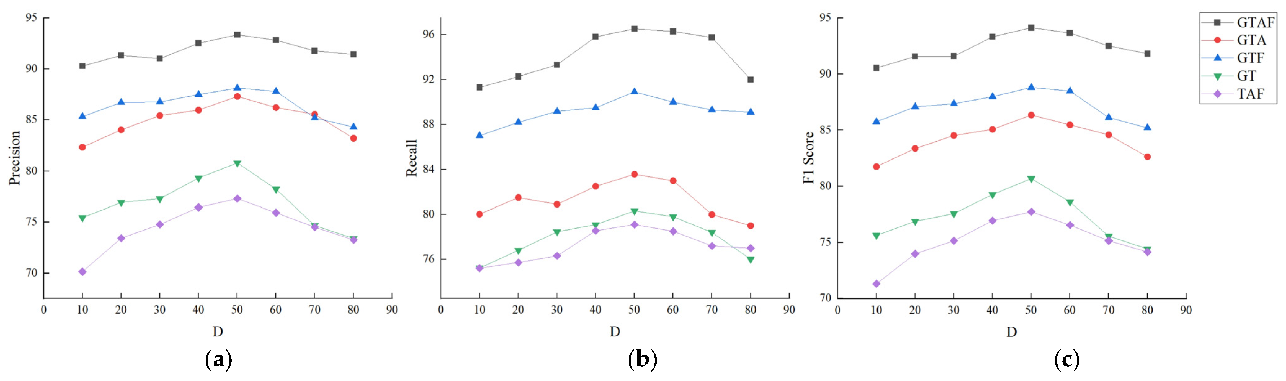
Ablation experiments: To verify the effect of each improvement feature of GTAF, some variant models, such as GTA, GTF, GT and TAF, were constructed by eliminating parts of features of GTAF. These variant models and GTAF were used on the datasets GFTD and SMAP, and their performances were compared.

(5)

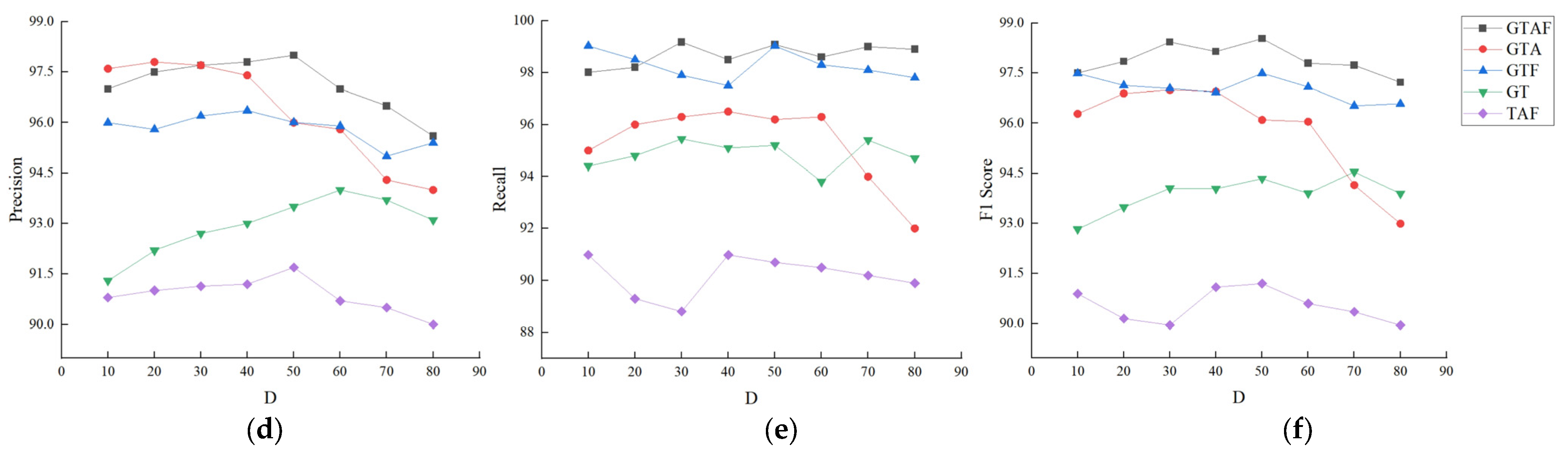
Parameter sensitivity: In order to study the parameter sensitivity of the model and explore the anomaly detection performance of the model under different model combinations, parameter sensitivity experiments were conducted. The parameter values of GTAF and the four variant models GTA, GTF, GT, and TAF on the datasets GFTD and SMAP are compared and analyzed.

3. Results and Discussion

3.1. Attribute Correlation of GFTD Dataset

The attributes of the GFTD dataset are described in detail in Section 2.3, and the attribute correlation heatmap is shown in Figure 6, which analyzes the correlation between the individual data attributes.

The Spearman correlation coefficient between TB3 and TB8 is 0.98, that between TB8 and TB9 is 0.91 and that between TB3 and TB9 is 0.89. It can be concluded that TB3, TB8 and TB9 are strongly correlated, i.e., the azimuth axis temperature is positively correlated with the elevation axis temperature and the cable temperature. The Spearman correlation coefficients between TB2 and TB3, TB2 and TB8, and TB2 and TB9 are 0.65, 0.62 and 0.6, respectively, and the signal antenna temperature is also correlated with other components. The Spearman correlation coefficients between the temperature attributes TB2, TB3, TB8, TB9 and the current attribute IB1, as well as the power state VB11, are smaller and show a relatively low correlation with the current attribute IB2 and no correlation with the heater attribute ZL5. As can be seen, several temperature attributes of the components are strongly correlated, while temperature is weakly correlated with attributes such as current or heater, and four temperature attributes are most relevant for the anomaly characterization.

3.2. Comparison Experiments for Anomaly Detection

3.2.1. Anomaly Detection for GFTD Dataset

For the GFTD dataset, the GTAF model proposed in this paper and other control models were used to undergo anomaly detection, and the results are shown in

Table 8. Results of anomaly detection analysis of GFTD dataset.

	Point Anomalies			Collective Anomalies			Association Anomalies
	P	R	F1	P	R	F1	P	R	F1
iForest	59.34	53.74	56.40	56.84	64.38	60.37	75.98	77.94	76.94
LOF	58.45	90.58	71.05	59.51	87.80	70.94	58.35	90.42	70.93
DAGMM	75.79	77.10	76.44	79.22	70.75	78.42	77.82	70.75	74.11
OmniAnomaly	88.67	91.17	89.89	83.34	94.49	88.57	77.97	95.86	85.99
LSTM-VAE	79.36	74.29	72.79	75.92	83.30	76.25	82.52	82.56	80.12
THOC	89.65	88.46	89.05	85.51	63.66	72.98	83.34	94.49	88.57
GDN	91.32	93.99	92.06	89.63	97.54	91.71	87.31	85.99	85.30
GTAF	92.28	96.66	94.12	92.52	99.03	94.17	93.70	93.90	93.80

, where the best results for the indicators are bolded.

As can be seen from Table 8, the precision of GTAF for GFTD data point anomalies is 92.28%, which is 55.51%, 57.87%, 21.75%, 4.07%, 16.28%, 2.93% and 1.05% higher than that of iForest, LOF, DAGMM, OmniAnomaly, LSTM-VAE, THOC and GDN, respectively. The precision of GTAF for collective anomalies was 92.52%, which is 62.77%, 55.47%, 16.79%, 11.02%, 21.87%, 8.20% and 3.22% higher than that of the other seven models, respectively. The precision of GTAF for correlation anomalies was 93.70%, which is 23.32%, 60.58%, 20.41%, 20.17%, 13.55%, 12.43% and 7.32% higher than that of the other seven models, respectively. The recall rates of GTAF for point anomalies, collective anomalies and correlational relationship anomalies were 96.66%, 99.03% and 93.90%, respectively, which were better than the recall rates of the other methods. Similarly, the F1 scores of GTAF of 94.12%, 94.17% and 93.80% for point anomalies, collective anomalies and associative relationship anomalies, respectively, outperformed the recall rates of the other seven methods.

From Table 8, it can be seen that the GTAF model has an advantage over the other methods in terms of detection accuracy in all metrics. In terms of stability, the GTAF model also has an advantage in detecting point anomalies, collective anomalies and correlation anomalies. In terms of sensitivity to correlation anomalies, the GTAF model has an outstanding advantage, with the other methods outperforming the other methods in terms of average F1 scores for correlation anomalies.

3.2.2. Anomaly Detection for SMAP Dataset

The results of the experiments of GTAF and the other seven time series anomaly detection methods on the SMAP dataset are shown in

Table 9. Comparison results of anomaly detection.

	Point Anomalies			Context Anomalies
	P	R	F1	P	R	F1
iForest	53.94	86.54	66.45	69.42	59.07	63.83
LOF	47.72	85.25	61.18	58.92	56.33	57.60
DAGMM	77.82	70.75	74.11	86.45	56.73	68.51
OmniAnomaly	89.02	86.37	87.67	83.34	81.99	82.66
LSTM-VAE	85.49	79.94	82.62	88.67	67.75	78.81
THOC	88.45	90.97	89.69	92.06	89.34	90.68
GDN	94.37	95.13	94.75	94.37	93.03	93.70
GTAF	96.92	93.13	94.99	96.36	94.10	95.27

.

As can be seen in Table 9, GTAF has a precision of 96.92% and 96.36% for point anomalies and contextual anomalies in SMAP data, respectively, a recall rate of 93.13% and 94.10%, and an F1 score of 94.99% and 95.27%, which are higher values than those of iForest, LOF, DAGMM, OmniAnomaly, LSTM- VAE, THOC and GDN, also demonstrating the performance of the GTAF model.

The experimental results show that GTAF outperforms the most popular multidimensional time series anomaly detection methods in terms of performance metrics for two anomaly types of the SMAP dataset, demonstrating that GTAF learns better temporal and inter-metric dependencies as well as local and global data features. The five modes, iForest, LOF, DAGMM, THOC, and LSTM-VAE, mainly model temporal dependencies and are more sensitive to local temporal dependencies in data. OmniAnomaly focuses more on inter-metric anomalies, and GDN has a good construction of inter-metric dependencies through graph neural networks, but neither of the above two approaches focuses enough on temporal dependencies. In summary, GTAF can learn the temporal and inter-dimensional dependencies of multidimensional time series more effectively, and can build richer feature representations in terms of data localization and data globalization, making up for the shortcomings of previous multidimensional time series anomaly detection methods that cannot capture multi-level information dependencies at the same time.

3.3. Evaluation for Anomaly Types

3.3.1. Anomaly Types in GFTD Dataset

It can be seen from the analysis in Section 3.1 that the correlation between the temperature attributes is strong and there are also certain correlations between the current attributes, so the attributes are divided into two sub-datasets with strong correlation: temperature and current. The three types of anomalies, point anomaly, collective anomaly and association anomaly, are experimented with, and the results are shown in Figure 7.

In Figure 7, the average F1 scores of the GTAF model were 93.55%, 92.81% and 93.90% for the three types of anomalies in the temperature dataset and 94.52%, 93.47% and 93.60% in the current dataset, respectively. For the point anomaly type and collective anomaly type, the F1 scores of the GTAF model in the temperature data set were smaller than those in the current dataset, indicating that temperature had some influence on the anomaly detection results and the temperature data were more volatile and correlated with the anomalies. However, for the association anomaly type, the F1 score of the GTAF model with the temperature dataset is higher than that in the current dataset, indicating that the GTAF model links the correlation between temperature attributes and captures the anomaly relationship between them, leading to a relatively higher F1 score.

3.3.2. Anomaly Types in SMAP Dataset

As described in Section 2.3, the dataset SMAP contains four levels of anomalies, L1, L2, L3 and L4, and two types of anomalies, point anomalies and contextual anomalies. The GTAF model performs anomaly detection for each level of data, and the results for the two types of anomalies in SMAP dataset are shown in Figure 8.

As can be seen from Figure 8, the GTAF model has a relatively high F1 score of 94% or more on all four sub-datasets for both the two types, point anomalies and contextual anomalies. For the type of point anomalies, GTAF performs well on the L3 product with an F1 score of 96.50%, better than the F1 scores of 95.52%, 94.64% and 94.93% of the GTAF model on the L1, L2 and L4 attributes, indicating that the GTAF model is better at capturing outliers and detecting data anomalies in the L3 attributes. In terms of contextual anomaly types, GTAF performed well on the L4 product with an F1 score of 96.30%, which is better than the F1 scores of 96.15%, 96.02% and 96.30% for the L1, L3 and L4 attributes, indicating that GTAF also performs well on data with strong contextual environmental correlations between spatio-temporal and soil moisture information such as L4.

3.4. Ablation Experiments

In order to further validate the rationality and effectiveness of the various modules of GTAF, the model proposed in this paper, ablation experiments of GTAF are performed using the full experimental dataset. The five models are listed as follows:

(1)

GTAF: the full model proposed in this paper, which uses the transformer model, the graph attention network and the multi-channel fusion module on the basis of GDN.

(2)

GTA: GTAF w/o F, i.e., the multichannel fusion module is removed from GTAF.

(3)

GTF: GTAF w/o A, i.e., the graph attention network is removed from GTAF.

(4)

GT: GTAF w/o AF, i.e., the graph attention network and multi-channel fusion module are removed from GTAF.

(5)

TAF: GTAF w/o G, i.e., the directed graph part for the correlation learning is removed from GTAF.

The results of ablation experiments of the above five models on the three performance metrics of P, R and F1 scores on the two experimental datasets are shown in

Table 10. Results of ablation experiments using GFTD dataset.

	Point Anomalies			Collective Anomalies			Association Anomalies
	P	R	F1	P	R	F1	P	R	F1
GTAF	92.28	96.66	94.12	92.52	99.03	94.17	93.70	93.90	93.80
GTA	87.31	85.99	85.30	82.52	82.56	80.12	87.11	82.18	87.53
GTF	88.08	96.10	91.16	84.03	91.18	86.51	82.35	85.47	82.99
GT	79.36	74.29	72.79	80.81	82.22	81.51	80.15	84.46	82.25
TAF	77.44	80.12	78.79	75.22	79.60	77.35	73.40	80.51	76.45

and

Table 11. Results of ablation experiments using SMAP dataset.

	Point Anomalies			Contextual Anomalies
	P	R	F1	P	R	F1
GTAF	96.92	93.13	94.99	96.36	94.10	95.27
GTA	94.77	92.64	93.69	92.25	90.99	91.66
GTF	95.82	92.33	94.04	93.11	93.28	93.19
GT	94.42	92.15	93.27	90.17	90.22	90.19
TAF	91.32	89.99	90.65	88.08	93.10	90.52

.

GTAF, the model proposed in this paper, improved the average F1 scores by 11.53% and 2.65% compared with the variant model GTA, 8.23% and 1.62% compared with the variant model GTF, 19.25 and 3.71% compared with the variant model GT, and 21.28% and 5.02% compared with the variant model TAF for both experimental datasets, respectively.

Compared with the model GT, the model GTA improved the average F1 scores on the two datasets by 6.93% and 2.92%, respectively, demonstrating that the graph attention network can capture dependencies and predicts well with the transformer model fusion, but the absence of the multichannel fusion module causes the model’s inability to fully learn global information.

Compared with the model GT, the model GTF improved the F1 scores on the two experimental datasets by 10.18% and 2.06% respectively, demonstrating that the adoption of the multichannel fusion module helps the model to learn richer and more effective features both globally and locally on the data.

The model GTF achieved an increase of 3.04% and 1.01% in the mean F1 scores on the two experimental datasets, respectively, compared to the model GTA, demonstrating that the multichannel fusion module is able to aggregate the results, resulting in better anomaly detection.

The performance of the model TAF is lower than that of GTAF, in both datasets, suggesting that the graph structure is also critical for the capture of anomalous data.

The analysis of the ablation experimental results demonstrates that, in the proposed model, GTAF, the combination of the multichannel fusion module and the transformermodel fused with the graph attention network can capture both local and global information dependencies of the multidimensional time series, thus exhibiting better anomaly detection performance.

3.5. Parameter Sensitivity

In the construction of the GTAF model, the parameter $D=d_{time}$ (vector size after timestamp encoding) has an important impact on the prediction part of the Transformer model and the graph attention mechanism. In order to investigate the parameter sensitivity of the model and to explore the anomaly detection performance of the model under different combinations of parameters, parameter sensitivity experiments are conducted in this paper. In this section, experiments are conducted for different values of the parameter D to verify its effect on the model.

The value interval of D in the experiments is set as (10, 80). The impact of the parameter D on the performances of the proposed GTAF model and the four ablation models on the two data sets were examined, and the experimental results are shown in Figure 9. Among them, GTAF indicates the proposed model, GTA indicates GTAF w/o F model, GTF indicates GTAF w/o A model, GT indicates GTAF w/o AF model and TAF indicates GTAF w/o G model.

In the dataset GFTD, the anomaly detection performance metrics of the five anomaly detection models trended upwards in the interval (10, 50) and peaked at a D value of 50; similarly, in the dataset SMAP, F1 scored best when D was in the interval (10, 50), and the anomaly detection F1 score slowly decreased when D was greater than 50. In the dataset GFTD, the performance metrics of the five anomaly detection models trended downwards in the interval (50, 80) and stabilize at (70, 80); in the dataset SMAP, the F1 score decreased when D was in the interval (50, 80). It is worth noting that all three indicators of the GTAF model remain at high levels in both datasets GFTD and SMAP.

After the description of the above details, we can explain this situation [44,45]. Sensitivity analysis was performed on three performance metrics: Precision, Recall and F1 score. The anomaly detection performance of each model initially improved as the D value increased because the input time series could not characterize the local contextual information well when D was too small. However, when the D value is too large, subtle local anomalies are more likely to be hidden in the large number of normal time points, which makes the anomaly detection performance decrease. The GTAF model performs better in all performance indicators when the D value is 50, so the D value of 50 is the most suitable for this experiment.

4. Conclusions

To improve the performance of anomaly detection for sensing data, a composite model, GTAF, is proposed in this paper, which is based on GDN, combining transformerwith a graph attention network and incorporating a multi-channel data fusion module. The proposed model, GTAF, captures the unique features of each time series using embedding vectors; then, it uses directed graphs to learn the dependencies between time series data, while the Transformer module fuses with the graph attention mechanism to predict the values using the graph deviation score to identify deviations in the learned relationships, and the deviation between the true and predicted values is the final score for anomaly judgement. The performance of the proposed GTAF model is examined using two datasets from unmanned systems, and outperforms other state-of-the-art methods, demonstrating the effectiveness of the design of GTAF.

However, anomaly detection for unmanned systems should be able to detect anomalies in real-time flight data, which the GTAF model did not fully investigate. Thus, for future directions of research in anomaly detection on real-time data, the lightweighting of the model and the optimization of internal structure of the model will be studied to increase the anomaly detection rate and reduce the false positive rate in order to meet a wide range of requirements for anomaly detection in unmanned systems.

References

1. Sun, X.C.; Chen, X.P. Design of UAV flight control system fault diagnosis expert system. In Equipment Manufacturing Technology; University of Wollongong: Wollongong, NSW, Australia, 2012; pp. 66–68. [Google Scholar]
2. Liu, H.Z. Research on Intelligent Diagnosis System of UAV Flight Control Fault Based on Machine Learning; University of Electronic Science and Technology of China: Chengdu, China, 2019; pp. 20–25. [Google Scholar]
3. Singh, S.; Murthy, T.V.R. An Expert System Based Sensor Fault Accommodation for Lateral Dynamics of Aircraft Models. Eur. J. Mol. Clin. Med. 2020, 7, 2904–2916. [Google Scholar]
4. Qing, L.Y. Research on Airplane Fault Prognosis and Diagnosis System Based on Flight Data; Nanjing University of Aeronautics and Astronautics: Nanjing, China, 2007. [Google Scholar]
5. Chen, M.; Pan, Z.; Chi, C.; Ma, J.; Hu, F.; Wu, J. Research on UAV Wing Structure Health Monitoring Technology Based on Finite Element Simulation Analysis. In Proceedings of the 2020 International Conference on Prognostics and System Health Management, Jinan, China, 23–25 October 2020; IEEE: Piscataway, NJ, USA; pp. 86–90. [Google Scholar]
6. Tan, J. Research on Fault Diagnosis Technology of Flight Control System Based on Analytical Model; Nanjing University of Aeronautics and Astronautics: Nanjing, China, 2020; pp. 12–15. [Google Scholar]
7. Melnyk, I.; Matthews, B.; Valizadegan, H.; Banerjee, A.; Oza, N. Vector autoregressive model-based anomaly detection in aviation systems. J. Aerosp. Inf. Syst. 2016, 13, 1–13. [Google Scholar] [CrossRef]
8. Liu, Z.C.; Guo, L.J. Fault detection technology for UAV control system based on hierarchical filtering algorithm. Comput. Meas. Control 2020, 28, 23–26. [Google Scholar]
9. Yang, X.Y.; Yang, J.; Zhang, W.Y.; Guo, X.F.; Yang, Q.; Dong, W. Measurement data fusion model of a turbofan engine. J. Aerosp. Power 2020, 35, 641–650. [Google Scholar]
10. Bronz, M.; Baskaya, E.; Delahaye, D.; Puechmore, S. Real-time fault detection on small fixed-wing UAVs using machine learning. In Proceedings of the 2020 AIAA/IEEE 39th Digital Avionics Systems Conference (DASC), San Antonio, TX, USA, 11–16 October 2020; pp. 1–10. [Google Scholar]
11. Yaman, O.; Yol, F.; Altinors, A. A Fault Detection Method Based on Embedded Feature Extraction and SVM Classification for UAV Motors. Microprocess. Microsyst. 2022, 94, 104683. [Google Scholar] [CrossRef]
12. Pan, P.F. Condition monitoring and fault diagnosis of aero engines based on test flight data. Propuls. Technol. 2021, 42, 2826–2837. [Google Scholar]
13. Lv, C.; Cheng, G.; Liu, Y.Q. Aero-engine fault data tagging based on BDPCA clustering algorithm. Vib. Shock 2020, 39, 35–41. [Google Scholar]
14. Pan, D.; Nie, L.; Kang, W.; Song, Z. UAV anomaly detection using active learning and improved S3VM model. In Proceedings of the 2020 International Conference on Sensing, Measurement & Data Analytics in the era of Artificial Intelligence (ICSMD), Xi’an, China, 15–17 October 2020; pp. 253–258. [Google Scholar]
15. Ahmad, A.; Zouhair, D. Using MLSTM and multioutput convolutional LSTM algorithms for detecting anomalous patterns in streamed data of unmanned aerial vehicles. IEEE Aerosp. Electr. Syst. Mag. 2022, 37, 6–15. [Google Scholar]
16. You, J.T.; Liang, J.; Liu, D.T. An Adaptable UAV Sensor Data Anomaly Detection Method Based on TCN Model Transferring. In Proceedings of the 2022 Prognostics and Health Management Conference, Turin, Italy, 6–8 July 2022; IEEE: Piscataway, NJ, USA; pp. 73–76. [Google Scholar]
17. Li, C.; Wang, B.H.; Tian, J.W.; Wang, R.X. Anomaly detection method for UAV sensor data based on LSTM-OCSVM. J. Chin. Comput. Syst. 2021, 42, 700–705. [Google Scholar]
18. Kim, J.; Kang, H.; Kang, P. Time-series anomaly detection with stacked Transformer representations and 1D convolutional network. Eng. Appl. Artif. Intell. 2023, 120, 105964. [Google Scholar] [CrossRef]
19. Saraswat, D.; Bhattacharya, P.; Zuhair, M.; Verma, A.; Kumar, A. AnSMart: A SVM-based anomaly detection scheme via system profiling in Smart Grids. In Proceedings of the 2021 2nd International Conference on Intelligent Engineering and Management (ICIEM), London, UK, 28–30 April 2021; pp. 417–422. [Google Scholar]
20. Dixit, P.; Bhattacharya, P.; Tanwar, S.; Gupta, R. Anomaly detection in autonomous electric vehicles using AI techniques: A comprehensive survey. Expert Syst. 2022, 39, e12754. [Google Scholar] [CrossRef]
21. Raza, A.; Tran, K.P.; Koehl, L.; Li, S. AnoFed: Adaptive anomaly detection for digital health using transformer-based federated learning and support vector data description. Eng. Appl. Artif. Intell. 2023, 121, 106051. [Google Scholar] [CrossRef]
22. Deng, A.; Hooi, B. Graph neural network-based anomaly detection in multivariate time series. Proc. Conf. AAAI Artif. Intell. 2021, 35, 4027–4035. [Google Scholar] [CrossRef]
23. Buchhorn, K.; Santos-Fernandez, E.; Mengersen, K.; Salomone, R. Graph Neural Network-Based Anomaly Detection for River Network Systems. arXiv 2023, arXiv:2304.09367. [Google Scholar]
24. Tang, C.; Xu, L.; Yang, B.; Tang, Y.; Zhao, D. GRU-Based Interpretable Multivariate Time Series Anomaly Detection in Industrial Control System. Comput. Secur. 2023, 127, 103094. [Google Scholar] [CrossRef]
25. Guo, H.; Zhou, Z.; Zhao, D.; Hung, P.C. H-Gdn: Hierarchical Graph Deviation Network for Multivariate Time Series Anomaly Detection in Iot. SSRN 2022, ssrn:4283684. [Google Scholar]
26. Vaswani, A.; Shazeer, N.; Parmar, N.; Uszkoreit, J.; Jones, L.; Gomez, A.N.; Polosukhin, I. Attention is all you need. In Advances in Neural Information Processing Systems; ACM: New York, NY, USA, 2017; p. 30. [Google Scholar]
27. Veličković, P.; Cucurull, G.; Casanova, A.; Romero, A.; Lio, P.; Bengio, Y. Graph attention networks. arXiv 2017, arXiv:1710.10903. [Google Scholar]
28. Liu, F.T.; Ting, K.M.; Zhou, Z.H. Isolation Forest. In Proceedings of the 2008 Eighth IEEE International Conference on Data Mining, Pisa, Italy, 15–19 December 2008; IEEE: Piscataway, NJ, USA, 2008; pp. 413–422. [Google Scholar]
29. Breunig, M.M.; Kriegel, H.P.; Ng, R.T.; Sander, J. LOF: Identifying density-based local outliers. In Proceedings of the 2000 ACM SIGMOD International Conference on Management of Data, Dallas, TX, USA, 15–18 May 2000; pp. 93–104. [Google Scholar]
30. Zong, B.; Song, Q.; Min, M.R.; Cheng, W.; Lumezanu, C.; Cho, D.; Chen, H. Deep auto encoding gaussian mixture model for unsupervised anomaly detection. In Proceedings of the International Conference on Learning Representations (ICLR), Vancouver, BC, Canada, 30 April–3 May 2018; pp. 1448–1460. [Google Scholar]
31. Su, Y.; Zhao, Y.; Niu, C.; Liu, R.; Sun, W.; Pei, D. Robust anomaly detection for multivariate time series through stochastic recurrent neural network. In Proceedings of the 25th ACM SIGKDD International Conference on Knowledge Discovery & Data Mining, Anchorage, AK, USA, 4–8 August 2019; pp. 2828–2837. [Google Scholar]
32. Cui, Z.; Ke, R.; Pu, Z.; Wang, Y. Stacked bidirectional and unidirectional LSTM recurrent neural network for forecasting network-wide traffic state with missing values. Transp. Res. Part C Emerg. Technol. 2020, 118, 102674. [Google Scholar] [CrossRef]
33. Tay, Y.; Dehghani, M.; Bahri, D.; Metzler, D. Efficient transformers: A survey. ACM Comput. Surv. 2022, 55, 1–28. [Google Scholar] [CrossRef]
34. Guo, S.; Lin, Y.; Wan, H.; Li, X.; Cong, G. Learning dynamics and heterogeneity of spatial-temporal graph data for traffic forecasting. IEEE Trans. Knowl. Data Eng. 2021, 34, 5415–5428. [Google Scholar] [CrossRef]
35. Xu, M.; Dai, W.; Liu, C.; Gao, X.; Lin, W.; Qi, G.J.; Xiong, H. Spatial-temporal transformer networks for traffic flow forecasting. arXiv 2020, arXiv:2001.02908. [Google Scholar]
36. Ba, J.L.; Kiros, J.R.; Hinton, G.E. Layer normalization. arXiv 2016, arXiv:1607.06450. [Google Scholar]
37. Optics and SAR Satellite Payload Retrieval. Available online: https://data.cresda.cn/#/2dMap (accessed on 5 February 2023).
38. Sridhar, A.; Suman, K.A. Beginning Anomaly Detection Using Python-Based Deep Learning, with Keras and PyTorch, 1st ed.; Tsinghua University Press: Beijing, China, 2020; pp. 3–6. [Google Scholar]
39. Hundman, K.; Constantinou, V.; Laporte, C.; Colwell, I.; Soderstrom, T. Detecting spacecraft anomalies using lstms and nonparametric dynamic thresholding. In Proceedings of the 24th ACM SIGKDD International Conference on Knowledge Discovery & Data Mining, London, UK, 19–23 August 2018; pp. 387–395. [Google Scholar]
40. Kingma, D.P.; Welling, M. Auto-encoding variational bayes. arXiv 2013, arXiv:1312.6114. [Google Scholar]
41. Park, D.; Hoshi, Y.; Kemp, C.C. A multimodal anomaly detector for robot-assisted feeding using an lstm-based variational autoencoder. IEEE Robot. Autom. Lett. 2018, 3, 1544–1551. [Google Scholar] [CrossRef]
42. Shi, X.; Chen, Z.; Wang, H.; Yeung, D.Y.; Wong, W.K.; Woo, W.C. Convolutional LSTM network: A machine learning approach for precipitation nowcasting. In Advances in Neural Information Processing Systems; ACM: New York, NY, USA, 2015; p. 28. [Google Scholar]
43. Shen, L.; Li, Z.; Kwok, J. Timeseries anomaly detection using temporal hierarchical one-class network. Adv. Neural Inf. Process. Syst. 2020, 33, 13016–13026. [Google Scholar]
44. Jain, K.; Saxena, A. Simulation on supplier side bidding strategy at day-ahead electricity market using ant lion optimizer. J. Comput. Cogn. Eng. 2023, 2, 17–27. [Google Scholar]
45. Saikia, L.C.; Sinha, N.; Nanda, J. Maiden application of bacterial foraging based fuzzy IDD controller in AGC of a multi-area hydrothermal system. Int. J. Electr. Power Energy Syst. 2013, 45, 98–106. [Google Scholar] [CrossRef]
Figure 1. Structure of the GTAF anomaly detection model.
Drones 07 00326 g001
Figure 2. Transformer model structure.
Drones 07 00326 g002
Figure 3. Multi-head attention mechanism.
Drones 07 00326 g003
Figure 4. Multi-channel data fusion.
Drones 07 00326 g004
Figure 5. Structure of Bi-LSTM network.
Drones 07 00326 g005
Figure 6. Correlation of attributes in GFTD dataset.
Drones 07 00326 g006
Figure 7. Anomaly detection by the GTAF model on two datasets.
Drones 07 00326 g007
Figure 8. Anomaly detection for different anomalies for four types of data.
Drones 07 00326 g008
Figure 9. Parameter sensitivity experiments for the five models. (ac): results of experiments on GFTD dataset. (df): results of experiments on SMAP dataset.
Drones 07 00326 g009aDrones 07 00326 g009b