Article

Online Motion Planning for Fixed-Wing Aircraft in Precise Automatic Landing on Mobile Platforms

1
School of Automation, Beijing Institute of Technology, Beijing 100081, China
2
Systems Engineering Research Institute, China State Shipbuilding Corporation, Beijing 100094, China
*
Author to whom correspondence should be addressed.
Drones 2023, 7(5), 324; https://doi.org/10.3390/drones7050324
Submission received: 30 March 2023 / Revised: 5 May 2023 / Accepted: 16 May 2023 / Published: 18 May 2023
(This article belongs to the Section Drone Design and Development)

Abstract

:
This paper proposes the creative idea that an unmanned fixed-wing aircraft should automatically adjust its 3D landing trajectory online to land on a given touchdown point, instead of following a pre-designed fixed glide slope angle or a landing path composed of two waypoints. A fixed-wing aircraft is a typical under-actuated and nonholonomic constrained system, and its landing procedure—which involves complex kinematic and dynamic constraints—is challenging, especially in some scenarios such as landing on an aircraft carrier, which has a runway that is very short and narrow. The conventional solution of setting a very conservative landing path in advance and controlling the aircraft to follow it without dynamic adjustment of the reference path has not performed satisfactorily due to the variation in initial states and widespread environmental uncertainties. The motion planner shown in this study can adjust an aircraft’s landing trajectory online and guide the aircraft to land at a given fixed or moving point while conforming to the strict constraints. Such a planner is composed of two parts: one is used to generate a series of motion primitives which conform to the dynamic constraints, and the other is used to evaluate those primitives and choose the best one for the aircraft to execute. In this paper, numerical simulations demonstrate that when given a landing configuration composed of position, altitude, and direction, the planner can provide a feasible guidance path for the aircraft to land accurately.

1. Introduction

Compared to copters, fixed-wing aircraft have many irreplaceable advantages, such as long endurance, high speed, large load, etc. However, they are required to take off and land on runways, whereas copters can perform these tasks vertically. To minimize the constraints created by the use of a runway, many methods have been designed to help fixed-wing aircraft reach the takeoff speed faster (e.g., catapult-assisted takeoff [1], vertical takeoff and landing (VTOL) [2]). Similarly, there are approaches that help fixed-wing aircraft land on short runways or even without runways (e.g., parachute landing and arrested landing [3]). However, most of those are suitable for small unmanned aerial vehicles (UAVs), whereas larger ones still require taxiing for takeoff and landing.
Automatic landing of fixed-wing aircraft on shorter runways is one of the most difficult multidisciplinary challenges, involving dynamics, navigation, and control engineering, because the complex transformation of energy, differential constraints, strict boundary constraints, etc., need to be addressed.
The conventional method is to design a conservative fixed gliding trajectory offline based on an aircraft’s performance and control the airplane to track the reference trajectory. The key aspect of this method is trajectory tracking. However, as the initial point is random and the environment is complex, the reference trajectory should be more flexible and adaptive. To this end, an automatic landing trajectory planner can be designed to fine-tune the trajectory online, which can ensure that aircraft land at a given point (also known as precise landing), reduce unnecessary aborting, and improve the quality of the landing path.
Unlike other robots (i.e., copters [4,5]), fixed-wing aircraft cannot come to a full stop midair because they have to maintain a high speed to generate lift. With their huge amount of inertia, airborne aircraft cannot brake at will unless the spoilers produce a limited amount of drag. In other words, the gravitational potential energy of the aircraft can only be released by its friction with air. Unlike holonomic robots (e.g., quad-rotors), it is difficult to directly formulate generation of the landing path as an optimization problem given the complex transformation of energy and nonholonomic constraints of fixed-wing aircraft.
Inspired by the practices of experienced pilots, this study proposes a novel approach in which the landing trajectory and velocity are adjusted automatically during the landing process. By estimating the distance between the current position and the target position, the planner will judge how to guide the aircraft to the target point more accurately while conforming to the strict constraints. If an aircraft is too high relative to a given touchdown point, the planner will command it to take a detour so as to consume excess gravitational potential energy. When it is at the appropriate height, the planner will navigate it back to the conventional landing path, which is aligned with the touchdown point. If it is too low, the planner will instruct it to reduce the flight path angle. Such a planner is composed of two parts: one is used to generate a series of alternative motion primitives, which are in line with the kinematic and dynamic constraints because they are generated by forward integration for a given interval of time, and the other is used to evaluate those primitives and select the one with the highest quality for execution. The evaluation criteria include heuristic time to the ideal touchdown point, the speed of the aircraft, and the position error between the conventional landing path and the current position. Of them, the first criterion is the most important. The heuristic time is estimated by the length of the Dubins path [6] which is made up of line segments and circular arcs. Although the Dubins path cannot be precisely tracked as its curvature is discontinuous, it takes the minimum turning radius into consideration, and the length of the Dubins path is very similar to the length of the actual trajectory. This study uses it to estimate the heuristic distance, as its length can be easily calculated.
Comparison with the existing literature: Path planning for car-like vehicles (i.e., nonholonomic vehicles) has been widely researched with a variety of methods (e.g., hybrid-A* [7], lattice planner [8,9,10]), but few of them can be directly used in fixed-wing aircraft because they fly in three dimensions. In addition, the above methods usually generate a smooth, obstacle-avoiding, energy-saving path in an obstacle environment while seldom taking the minimum speed constraint into account. Thus, methods for fixed-wing aircraft should be specially designed. A solution for fixed-wing aircraft by combining Dubins path with the rapidly exploring random tree (RRT) algorithm [11,12] was studied in [13], but the focus was obstacle avoidance and the strict endpoint constraints were not addressed. A curvature-continuous path was generated by linking two circles with a Pythagorean-hodograph quintic Bezier curve in [14], and it focused on the feasibility of the path in a 2D workspace where the altitude of the path stays unchangeable. Compared with common autonomous navigation (i.e., navigation based on waypoints), automatic landing is much more complex and has not been completely researched. Multi-copters landing on a mobile platform were studied in [15,16,17,18,19], but the landing principles of copters and fixed-wing UAVs are fundamentally different. Therefore, methods for fixed-wing UAVs should be redesigned. Autolanding of fixed-wing aircraft on a moving ground vehicle was studied in [20], but it focused on the cooperative control of the two vehicles, and the aircraft had little flexibility, i.e., the initial and target states of the aircraft and the moving platform were strictly constrained. Path planning for emergency landing (under engine failure) was studied in [21,22,23], but the trajectories were generated only once and the focus was on unpowered glides. Thus, those methods are not applicable to moving platforms. Our study works for emergency landings because the energy conversion relationship is essentially the same. The aircraft can arrive at a target point as long as the point is within reach of an unpowered glide. An adaptive algorithm for fixed-wing UAV autolanding on an aircraft carrier was presented in [24], but the adjustment was limited to the vertical plane. Thus, the speed constraint still cannot be addressed effectively. Various controllers for tracking gliding trajectory were studied in [25,26,27], but none of them focused on changing the shape of the landing path. In references [3,28], cubic spiral curves for landing were generated only at the beginning of the landing, but the planner in this study runs at a high frequency and generates motion primitives using a method similar to the dynamic window approach (DWA) in [29,30]. However, the evaluation criteria (i.e., cost function) in this study are redesigned and completely different from DWA. DWA is used in many nonholonomic robots for its strength in dealing with obstacles. This study does not take obstacles into consideration, but differential constraints are fully considered and each primitive can be tracked precisely and smoothly.
The contribution of this study is summarized as follows:
  • This study proposes an idea to solve the automatic landing problem by combining a motion planner with a controller. The planner focuses on the reasonability and feasibility of the landing trajectory, whereas the controller focuses on precising tracking of the glide path. To the best of our knowledge, this is the first time that a method is presented for consuming excess energy with a short deviation from the conventional glide path before reentering the path. The proposed method is radically different from the existing methods, which order the aircraft to abort and retry as soon as some strict constraints are violated due to the limited flexibility.
  • An efficient algorithm for trajectory generation online is proposed for precise automatic landing on a fixed or moving platform with flexibility for adjustment. Based on the algorithm, the planner can guide the aircraft as an experienced pilot would based on their understanding of the aircraft’s performance.
The paper is organized as follows. Section 2 states the problem and defines the scope of the work. Section 3 describes the theory, including the fixed-wing aircraft motion model, the DWA algorithm, and the evaluation criteria. Section 4 presents simulation results. Finally, Section 5 analyzes the main results and summarizes this study.

2. Problem Statement

In this study, we seek to guide a fixed-wing aircraft from an initial flight state to a given touchdown point. The overarching goal is to control the aircraft from any initial configuration (altitude, heading angle, speed, etc.) to a given target configuration. Although we focus on small UAVs ranging from 1–100 kg in mass and their speeds are relatively low ranging from 10–40 m/s, the automatic landing planner should be made as general as possible so that it can be widely used for any other fixed-wing aircraft, as long as the same kinematic model is followed.
The kinematic model used in this study is the Dubins airplane motion model [31], which will be presented in the next section. The Dubins airplane model is an extension of the Dubins car, which follows the basic behavior of Ackerman-steered vehicles in a 2D plane. Therefore, this study is not suitable for helicopters and multi-copters.
The basic parameters of the aircraft are always known beforehand, including the best gliding ratio, the stall speed, the maximum level flight speed, the maximum safe roll angle and roll rate, the minimum turning radius, etc. Here, these parameters can be obtained easily from experienced pilots or the manufacturers.
In addition, we assume that the aircraft already has a low-level flight controller to track the commands from the planner. The controller can adjust the aircraft to the target speed and angular velocity. Furthermore, information collected by the sensors (the state of the aircraft), such as position, attitude, etc., is available at a high refresh frequency.
It is assumed that there are no obstacles near the touchdown point. So, the study does not take any obstacles into account. Furthermore, if the touchdown point is moving, we assume that the moving platform is a cooperative vehicle (i.e., the states of the platform should be known), and it moves with a fixed direction and forward only. In addition, the speed of the moving platform should be smaller than that of the aircraft. The assumption that the movement of the platform is constrained is reasonable because it is too difficult for a nonholonomic high-speed aircraft to capture orthogonal movement. The flare phase is left for future work.

3. Theory and Algorithm

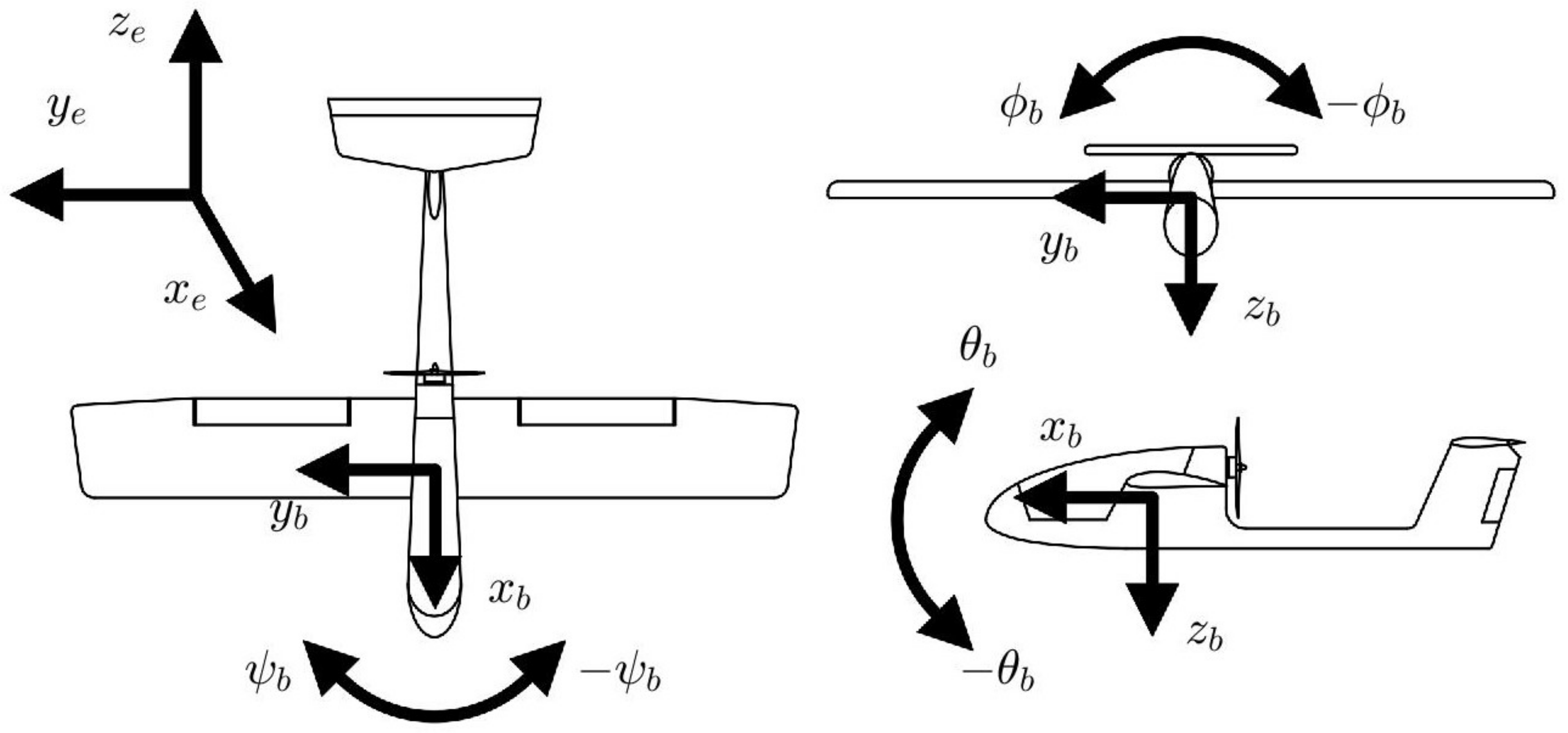
3.1. Coordinate Systems and Kinematic Model

As shown in Figure 1, two coordinate systems are used in this study: (1) the body frame F b and (2) the earth frame F e . To follow the convention, the body frame is fixed at the center of gravity of the aircraft, and the axes are x b forward, y b right, and z b down. The earth frame is considered as a fixed inertial frame with x e east, y e north, and z e up. The roll angle ϕ is expressed as the angle between the body’s y-axis y b and the earth plane ( x e , y e ), the pitch angle θ is expressed as the angle between the body’s x-axis x b and the earth plane ( x e , y e ), and the yaw angle ψ is expressed as the angle between the body’s x-axis x b and the earth’s x-axis x e .
A simplified kinematic model called the Dubins airplane is used in this study [31], and it maintains generality to most of fixed-wing aircraft. The Dubins airplane is often used in path planning for fixed-wing aircraft and it is an extension of the Dubins car. In the Dubins airplane, the roll angle is analogous to the steering angle of a ground vehicle, and the height is considered separately. In addition, the Dubins airplane assumes that the airspeed V is the same as the ground speed, the heading angle (yaw angle) ψ is the same as the course angle, and the flight path angle γ is the same as the air mass reference flight path angle [25]. The hypotheses of Dubins airplane may fail under complicated wind conditions or in an agile flight. However, the outputs of the planner are the linear speed and angular velocity of the aircraft, and the wind interference can be suppressed by the low-level flight controller.
The coordinated turn condition gives the relationship between the heading angle ψ and the roll angle ϕ , i.e., ψ ˙ = g V tan ( ϕ ) , where g is the gravitational acceleration.
The Dubins airplane kinematic model is expressed as
x ˙ = V cos ( ψ ) cos ( γ ) , y ˙ = V sin ( ψ ) cos ( γ ) , z ˙ = u z , ψ ˙ = ω ,
where V [ V min , V max ] , V min is the stall speed, V max is the maximum level speed, γ = arctan ( u z V ) , γ [ arctan ( u z , min V ) , arctan ( u z , max V ) ] , u z is the bounded climb and sink rate, u z [ u z , min , u z , max ] , ω is the bounded angular rate, and
ω = ψ ˙ = g V tan ( ϕ ) , ω [ g V tan ( ϕ max ) , g V tan ( ϕ max ) ] ,
in which ϕ max is the maximum roll angle.
As in Equation (2), the planner sends a target ω to the low-level controller, then the controller tracks the roll command ϕ c , i.e., ϕ c = arctan ( V ω g ) .
In an ideal unpowered slide, the gravitational potential energy is converted into kinetic energy, which is eventually dissipated by friction with air. In this scenario, the aircraft is in a stable state, i.e., D = m g sin ( γ i ) , V = V i , where D is the integrated resistance, m is the mass of the aircraft, γ i is the ideal glide path angle, and V i is the ideal touchdown speed. In motion planning for an automatic landing aircraft, we should get as close to γ i and V i as possible; then, the aircraft can land safely and save energy. It is assumed that either in a straight glide or a turning glide, the γ i and V i are constant, and they are known beforehand.
Dubins paths consist of line segments and circular arcs. The circular arcs can have different radii; however, the radii are constrained by the aircraft’s performance, i.e., there is a minimum turning radius. In a circular motion, we have
r = V ω .
Combining Equations (2) and (3), we obtain
r = V 2 g tan ( ϕ ) , r min = V 2 g tan ( ϕ max ) ,
where r min is the minimum turning radius when the roll angle ϕ reaches the maximum ϕ max .
A Dubins car is used to describe the kinematic model of the carrier, i.e.,
x f ˙ = V f cos ( ψ f ) , y f ˙ = V f sin ( ψ f ) , ψ f ˙ = ω f ,
where V f [ 0 , V f max ] is the speed of the carrier, V max is the maximum speed, ψ f is the heading angle, and ω [ ω f min , ω f max ] is the bounded angular rate.

3.2. Algorithm Description

Fixed-wing aircraft are typical nonholonomic vehicles, and they are constrained by a minimum turning radius. The actuators have mechanical restrictions that affect the performance of the aircraft, e.g., acceleration, angle, and acceleration. For safety reasons, the attitude angles are restricted in certain ranges. In this paper, DWA is used to generate motion primitives for fixed-wing aircraft with consideration of those constraints; however, the score function of DWA has been redesigned to meet the requirements of the study. The flowchart of modified DWA is shown in Figure 2.

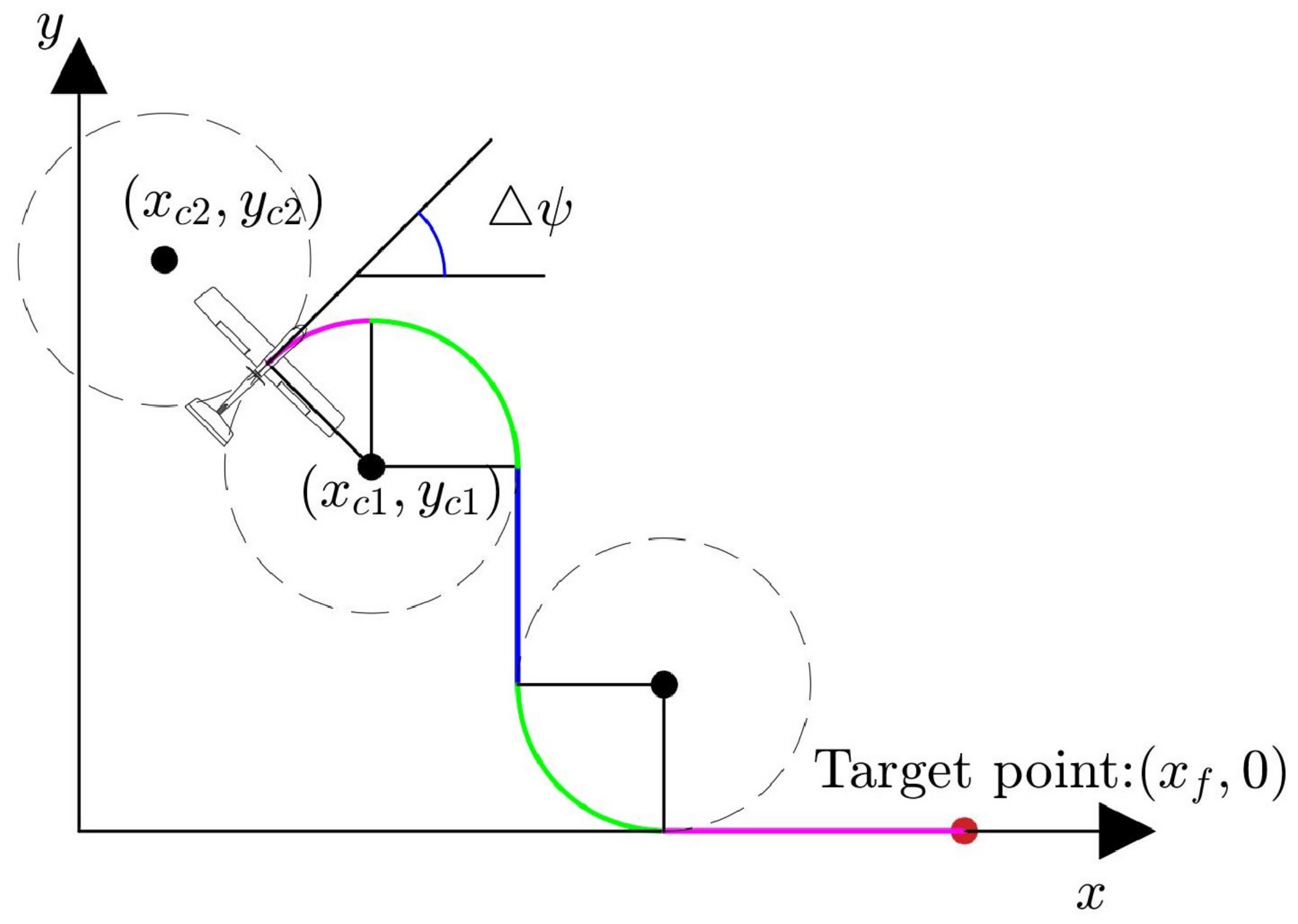
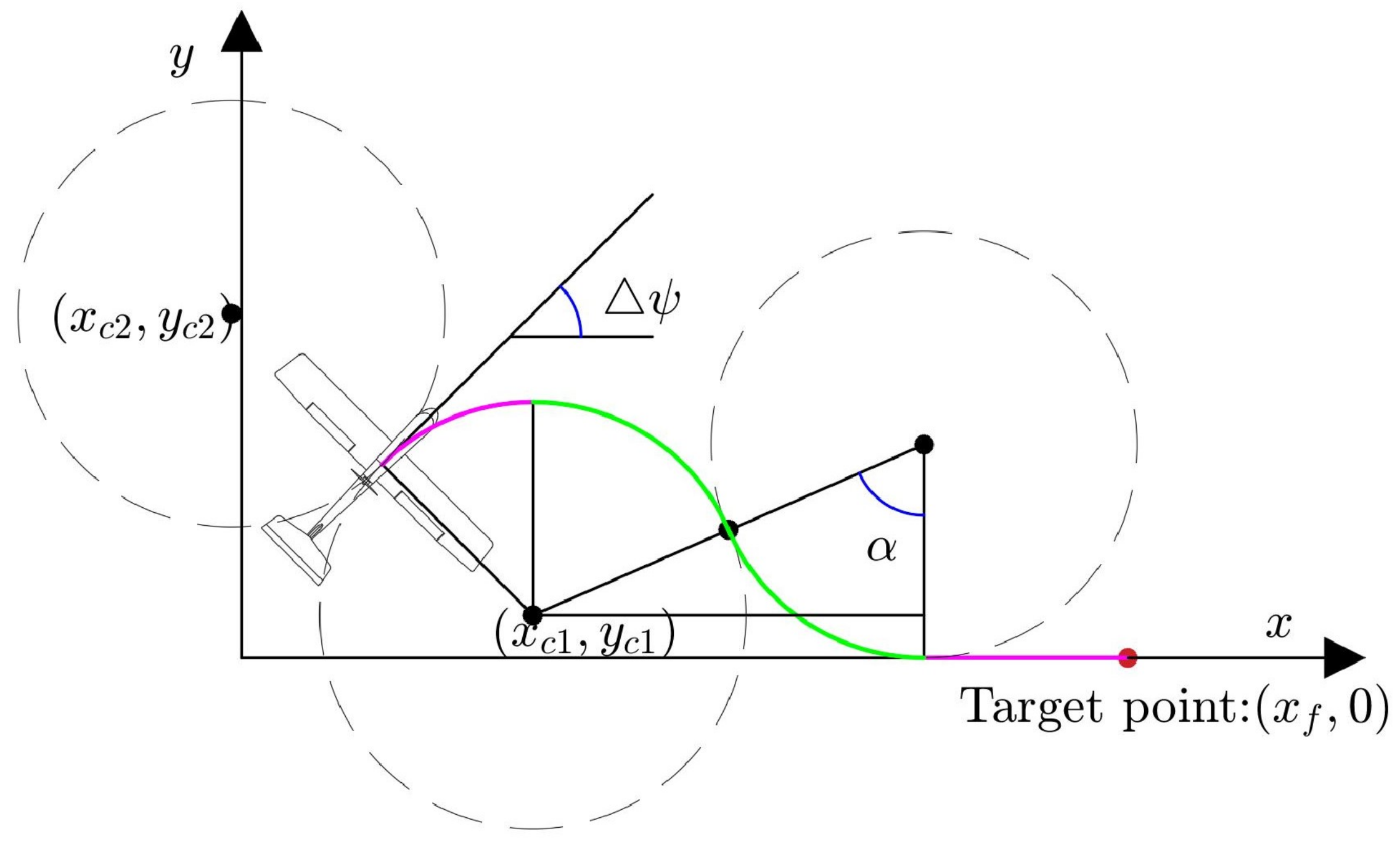
3.2.1. Motion Primitives

The dynamic windows based on the assumption that obstacles are not considered are shown in Figure 3. These windows are defined by constraints of an aircraft in a velocity space. The window V s drawn by a solid line can be obtained by the ultimate performance of the aircraft. Therefore, the window is
V s = { V , ω | V min V V max , ω min ω ω max } ,
and V s ensures that commands sent to the low-level controller can be reached.
The window V d indicated by the dashed line is defined by current velocities and maximum/minimum acceleration. The window is defined as
V d = { V , ω | V k + a min t V V k + a max t , ω k + α min t ω ω k + α max t } ,
where V k is the current velocity, ω k is the current turning rate, T is the integral time of forward simulation, a min and a max are the minimum/maximum linear accelerations in level flight, and α min and α max are the minimum/maximum angular accelerations. V d ensures that the target velocity and turning rate conform to the linear acceleration and angular acceleration restrictions of an aircraft.
The window V a in an oblique line corresponds to the condition that the aircraft slides to the touchdown point without a circle. That means the angle ψ of the difference between the heading angle of the aircraft and the direction of the runway should satisfy π 2 ψ π 2 . Thus, V a is determined by
V a = { V , ω | V min V V max , π 2 ψ t ω π 2 ψ t } .
This window ensures that the aircraft will not turn back and will close in the touchdown point.
Finally, the window V r is overlapped with these windows, i.e.,
V r = V s V d V a .
The commands for automatic landing are sampled from V r by discretizing the V and ω .
As shown in Figure 4, a series of motion primitives are generated by “forward simulation”. For each feasible input, we simulate the trajectory for T with the Dubins airplane kinematic model (i.e., Equation (1)). Furthermore, the end states of the motion primitives will be evaluated, then a primitive with the highest quality will be chosen for execution.

3.2.2. Evaluation Criteria

The score function (i.e., the cost function) is defined as
J = λ y J y + λ V J V + λ t J t ,
where J y is the orthogonal distance to the vertical plane which contains the runway; J V is the speed penalty function; J t is the heuristic time penalty function; and λ y , λ V , and λ t are weights.
The first term J y penalizes the path-tracking error; then, the primitive close to the runway tends to be chosen. The second term J V penalizes the speed, and the primitive with lower speed tends to be chosen because the lower the touchdown speed of the aircraft the better, as long as it does not stall. The third term J t penalizes the heuristic time to the touchdown point; then, the primitive with the appropriate heuristic time tends to be chosen.
With respect to heuristic time, we use the Dubins path [6] to link the current position and the touchdown position regardless of the altitude. Dubins path takes the minimum turning radius constraint into account in path planning for nonholonomic constrained robots, and it is made up of line segments and circular arcs. In an autolanding scenario, a fixed-wing aircraft is expected to line up with the runway as quickly as possible as long as the gliding distance is enough to reduce altitude. According to the initial state of the aircraft relative to the runway, three kinds of Dubins links are used to navigate the aircraft to line up with the runway. Intuitively, the aircraft will fly to the runway perpendicularly if it is far away from the runway, namely, it will fly in a line segment between two circular arcs (shown in Figure 5). Accordingly, there is no need for a line segment to connect two arcs if the aircraft is near the runway in Figure 6 and Figure 7. In Figure 6, the aircraft lines up with the runway using a right–left turn, and in Figure 7, the aircraft lines up with the runway using a left–right turn. By geometric computation, we can obtain the heuristic distance between the initial pose and the touchdown pose. For brevity, we set that the touchdown point is on the x-axis and moving to the positive x-axis without any loss of generality. Either the aircraft is above the x-axis or under the x-axis, and the two scenarios are similar. Here, we take the situation where “the aircraft is above x-axis” as an example, and the results of the scenario that the aircraft is under the x-axis will be given shortly.
The heuristic distance d H in Figure 5 is
d H = ( ψ + π ) R + y c 1 3 R + x f x c 1 , y c 1 > R ,
where x c 1 = x + R sin ( ψ ) , y c 1 = y R cos ( ψ ) , ( x , y ) is the current position of the aircraft, points ( x c 1 , y c 1 ) and ( x c 2 , y c 2 ) are the centers of the circular arcs, R is the radius of circular arcs of Dubins path, ( x f , 0 ) is the target touchdown point, and the ψ is the angle difference between the heading angle of the aircraft and the direction of the runway in earth frame.
The heuristic distance in Figure 6 is
d H = ( ψ + 2 α ) R + x f x c 1 4 R 2 ( R y c 1 ) 2 , y c 1 R , y c 2 R ,
where α is the central angle of the arc of the tangent Dubins circle and the x-axis, x c 2 = x R sin ( ψ ) , y c 2 = y + R cos ( ψ ) = R , α = arccos ( R y c 1 2 R ) ; the other variables are defined the same as Equation (11).
The heuristic distance in Figure 7 is
d H = ( ψ + 2 β ) R + x f x c 2 2 R sin ( β ) , y c 1 R , y c 2 < R ,
where β is the central angle of the arc of the tangent Dubins circle and the x-axis, β = arccos ( R + y c 2 2 R ) , and the other variables are defined as in Equations (11) and (12).
Similarly, when “the aircraft is under the x-axis”, we give the results directly, i.e.,
d H = ( ψ + π ) R y c 1 3 R + x f x c 1 , y c 1 < R , ( ψ + 2 α ) R + x f x c 1 4 R 2 ( R + y c 1 ) 2 , y c 1 R , y c 2 R , ( ψ + 2 β ) R + x f x c 2 2 R sin ( β ) , y c 1 R , y c 2 > R ,
where
x c 1 = x R sin ( ψ ) , y c 1 = y + R cos ( ψ ) ,
x c 2 = x + R sin ( ψ ) , y c 2 = y R cos ( ψ ) ,
α = arccos ( R + y c 1 2 R ) , β = arccos ( R y c 2 2 R ) .
An ideal glide time implies that the aircraft arrives the touchdown point when its altitude descends to zero exactly. So, the ideal glide time t i is defined as
t i = z u z = z V s i n ( γ ) .
The heuristic time t H is the length of time that it will take the plane to rise above the landing point regardless of the altitude. In order to autoland more precisely, the motion primitive with its heuristic glide time t H the closest to the ideal glide time t i tends to be chosen for execution.
If the target touchdown point is fixed, then the heuristic time t H is
t H = d H V cos ( γ ) .
We note that 2D Dubins paths are used, and accordingly, the projection speed V cos ( γ ) on the earth plane ( x e , y e ) will be used to compute the heuristic time.
Further, if the target touchdown point is moving, then we have
t H = d H V cos ( γ ) V f ,
where V f is the instantaneous speed of the touchdown point.

3.2.3. Algorithm Implementation

We use Dubins airplane motion model (i.e., Equation (1)) for simulation and generation of the primitives. The states of the fixed-wing aircraft are refreshed by x k + 1 = f ( x ( k ) , u ( k ) , t ) , i.e.,
x y z ψ k + 1 = 1 0 0 0 0 1 0 0 0 0 1 0 0 0 0 1 x y z ψ k + cos ( ψ ) cos ( γ ) t 0 sin ( ψ ) cos ( γ ) t 0 sin ( γ ) t 0 0 t k V ω k ,
where [ x , y , z , ψ ] T is the state of the aircraft, [ V , ω ] T is the input of the aircraft, and t is the sampling period.
Similarly, the states of the fixed or moving touchdown point are refresh by Equation (5), i.e.,
x f y f ψ f k + 1 = 1 0 0 0 1 0 0 0 1 x f y f ψ f k + cos ( ψ f ) t 0 sin ( ψ f ) t 0 0 t k V f ω f k ,
where [ x f , y f , ψ f ] T is the state of the touchdown point, and [ V f , ω f ] T is the input. Combining this with the assumption that the touchdown point is on the x-axis and moves towards the positive x-axis, we obtain y f = 0 , ψ f = 0 , and ω f = 0 , and the problem is greatly simplified.
If the heuristic time t H is longer than the ideal glide time t i , the aircraft will reduce u z to glide longer; in other words, the aircraft cannot perform an ideal glide to land, and the engine is working when sliding. With respect to the scenario where the heuristic time t H is shorter than the ideal glide time t i , this scenario implies that if the aircraft slides to the touchdown point directly, then either going over speed or flying over the touchdown point will doubtlessly happen. In this scenario, the aircraft should take a detour to consume energy. That means the aircraft should reduce its altitude before reaching the touchdown point. In order to avoid the problem where the aircraft may take an unreasonable or unnecessary detour frequently, we set a range [ t r , 0 ] in which the aircraft will adjust the pose only by adjusting speed V. Combining with Equations (15) and (17), we obtain the three terms in the penalty function. If t H t i 0 , the aircraft will try to get close to the line glide path, overlooking J t , i.e.,
J y = | y | , J V = V , J t = 0 .
If t H t i < t r , the aircraft will take a detour and overlook the tracking error, i.e.,
J y = 0 , J V = V , J t = | t H t i | .
If t r t H t i < 0 , i.e., the altitude error is so small that it can be adjusted only by the speed V, then we have
J y = | y | , J V = 0 , J t = 0 .
After scoring the primitives, we should normalize J y , J V , J t , respectively, i.e.,
J μ ( i ) = J μ ( i ) i = 1 n J μ ( i ) , μ { y , V , t } .
Now we consider how to obtain the target descent speed.
As shown in Figure 8, if the aircraft’s altitude is too high to glide to the touchdown point directly, it will circle to lose altitude. In other words, the aircraft can slide to the touchdown point without a circle and the altitude of the starting point H s should satisfy H s ( d H + 2 π R ) tan ( γ i ) . Furthermore, if H s does not meet the inequality condition, the aircraft only needs to circle to lose altitude. This study focuses on the final stage of the automatic landing. Therefore, the aircraft simply needs to move in a serpentine course to lose the extra altitude after starting the final gliding stage.
In Figure 9, if the aircraft has enough distance to lose altitude, namely, V cos ( γ i ) t i < d H + V f t i , where t i = H s V cos ( γ i ) , then the path angle command γ c should be reduced to accommodate the distance, i.e.,
γ c = arctan ( H s d H + t H V f ) ,
where t H = d H V cos ( γ ) V f ; here, the fact that “ γ is a small value” enables us to assume that t H = d H V V f .
Accordingly, if the aircraft has insufficient distance to lose altitude, i.e., V cos ( γ i ) t i d H + V f t i , then the aircraft should take a detour to lose more altitude. In addition, the aircraft should try to lose altitude as quickly as possible, i.e., it should take the ideal landing path angle γ i as the path angle command; then, we have
γ c = γ i .

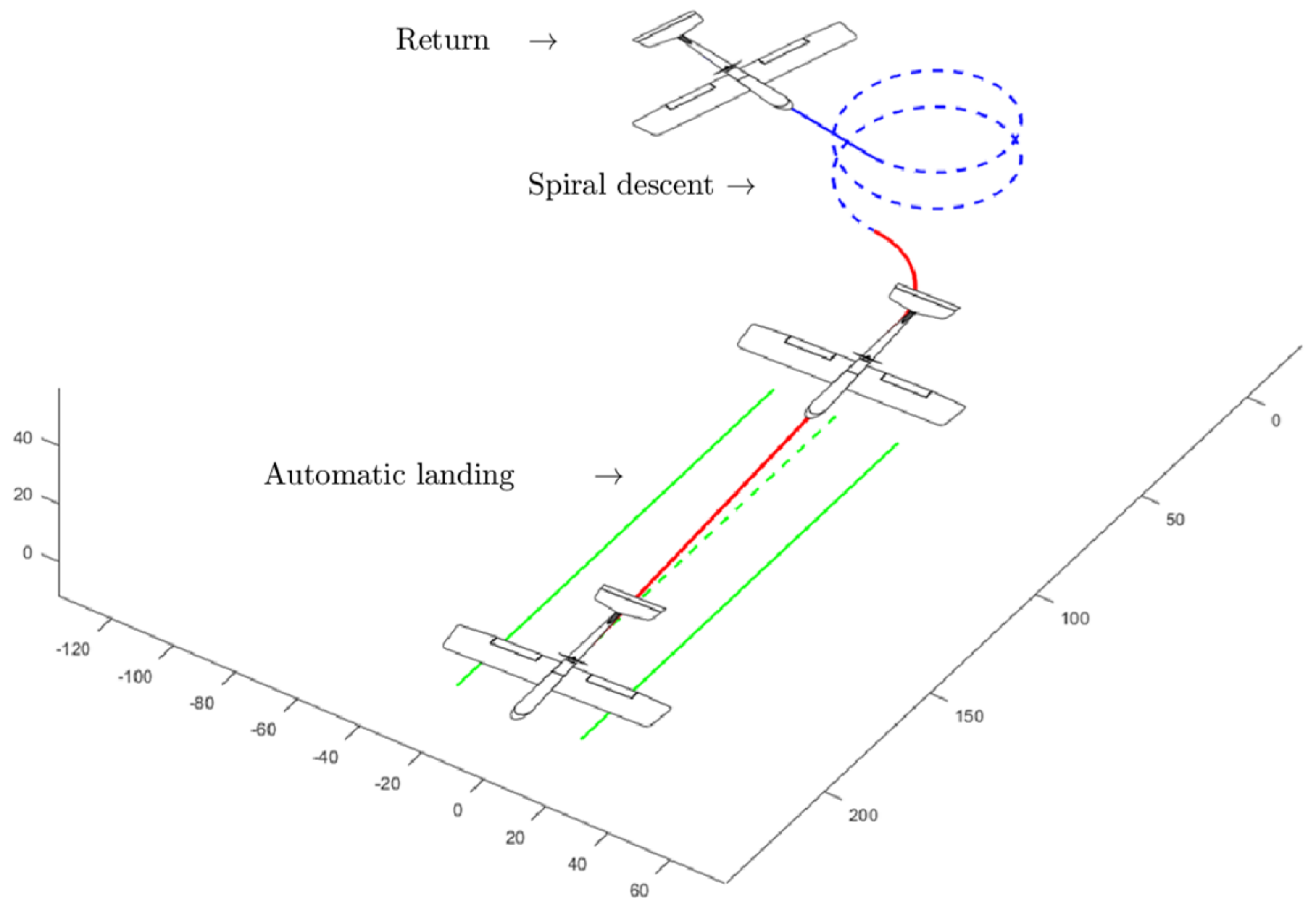
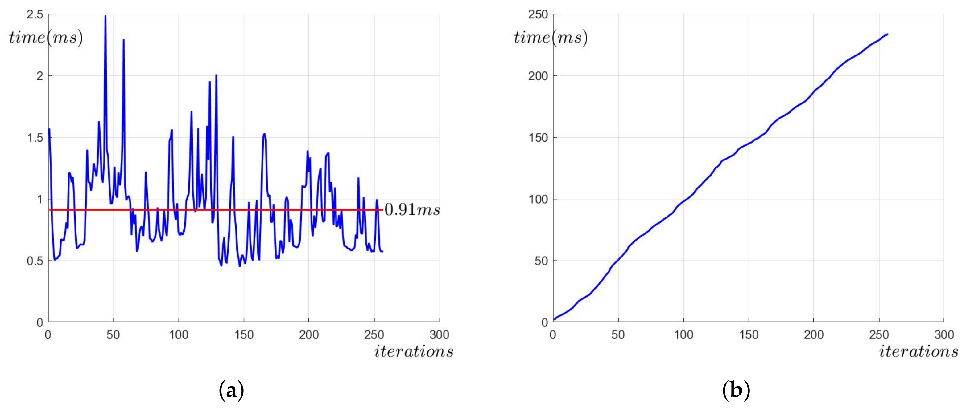
4. Numerical Simulation

In the numerical simulation, we choose a fixed-wing UAV (YuanZheng-6) (shown in Figure 10) as a reference to design the simulation parameters. The characteristics and performance of the aircraft are shown in Table 1, and Table 2 shows the parameters used in the simulation.
A flowchart of the numerical simulation is shown in Figure 11. Before reaching the touchdown point, the planner is always estimating how to get close to the target point more precisely and choose the best primitive to execute.
Numerical simulations were carried out in MATLAB on an Intel i7 laptop. As shown in Figure 12, an iteration takes only about 1 ms. In this study, the sampling time is 100 ms.
In Figure 13, the airplane started from a point (0 m, 50 m, 50 m) with different heading angles from π 2 rad to π 2 rad with an interval π 4 rad, aiming at landing on a fixed touchdown point (300 m, 0 m, 0 m). In addition, the heading angle of the aircraft at the moment of touchdown should be consistent with the runway (i.e., positive x-axis), and the aircraft should not have either a lateral speed or a lateral acceleration. The results show that the aircraft landed with high quality, and its speed and angular rate were bounded strictly during the landing procedure.
Another set of simulation results is shown in Figure 14. The aircraft started from a point (0 m, 50 m, H s ) with the heading angle 0 rad, where the initial altitudes H s were 36∼48 m with an interval 3 m. Furthermore, the target touchdown point was (600 m, 0 m, 0 m). The results show that if the initial altitude of the aircraft was too high to land directly, the planner would guide the aircraft to lose altitude, and if the initial altitude of the aircraft was appropriate to the heuristic distance, the planner would guide the aircraft to land directly.
A moving target touchdown point was used to simulate the automatic landing procedure in Figure 15. The target point started moving from point (400 m, 0 m, 0 m), and its speed was in the range 8∼16 m/s with an interval 2 m/s. The aircraft started from point (0 m, 20 m, 45 m) and had a heading angle of 0 rad. The simulation results show that our algorithm is effective for granting fixed-wing aircraft the ability to land on a moving platform (e.g., aircraft carrier).

5. Analysis and Conclusions

The paper proposes the novel idea that the automatic landing problem of fixed-wing aircraft may be better solved by coupling a motion planner with a conventional controller. Conventional methods pay more attention on tracking the conservative landing path accurately, and rarely operate similar to human pilots who often manipulate the aircraft to fly extra turns to fine-tune the predictive touchdown point. A sampling-based algorithm is implemented to verify if the idea is feasible. The sampling process of the algorithm is similar to DWA, but a fully redesigned cost function is proposed to meet the requirement of precise autolanding, and a complete simulation is carried out to demonstrate the feasibility of the algorithm.
In the numerical simulations, the aircraft started landing from various initial poses and ended landing on a fixed or moving target point. By choosing a series of appropriate primitives to execute, the planner was able to guide the aircraft to land precisely.
Numerical simulation results show that the method based on motion planning is feasible. A Dubins airplane kinematic model was used in the simulation, including computation of the heuristic time and simulating the trajectories that the aircraft had flown. The trajectories of the aircraft was reasonable and feasible, because the dynamics of the fixed-wing aircraft is taken into account when motion primitives were generated. Dubins path was used to predict the touchdown time, then the planner was able to judge whether the aircraft should return to the conventional glide path or to continue flying away to lose more altitude.
Precise autolanding involves not only landing on short runways, but also rope/net recovery. The latter is suitable for small UAVs in the range of tens of kilograms in mass with limited kinetic energy. The study is suitable for those recovery schemes. Moreover, the idea proposed in this study might be useful for UAV swarm recovery by some improvements. In scenarios with a lack of recovery facilities or workers, we may expect/need the UAVs to land orderly with a given interval time (e.g., 5 min). The algorithm in this study can be modified easily to meet the expectation of assigning a landing time. However, some approaches for collision avoidance and coordinating landing sequence should be studied.

Author Contributions

Conceptualization, J.L. and S.W.; methodology, J.L.; software, J.L.; validation, J.L., S.W. and B.W.; formal analysis, J.L. and B.W.; writing—original draft preparation, J.L.; writing—review and editing, B.W.; supervision, S.W.; project administration, S.W.; All authors have read and agreed to the published version of the manuscript.

Funding

This research received no external funding.

Data Availability Statement

The data that support the findings of this study are available from the corresponding author J.L. upon reasonable request.

Conflicts of Interest

The authors declare no conflict of interest.

Abbreviations

The following abbreviations are used in this manuscript:
x b , y b , z b axes of body-fixed coordinate system
x e , y e , z e axes of the inertial coordinate system
x , y , z position of the aircraft
θ , ψ , ϕ pitch, yaw (heading), and roll angle
x , u state vector, input vector
V , ω speed, angular rate of the aircraft
V k , ω k current velocity and angular rate
H s altitude of start point of automatic landing
α min / α max minimum/maximum angular acceleration
γ flight path angle
γ i , V i ideal glide path angle, ideal touchdown speed of automatic landing
γ c path angle command
ϕ c roll angle command
u z climb and sink rate
mmass of the aircraft
ggravitational acceleration
alinear acceleration
rturning radius of the aircraft
Rradius of circular arcs of Dubins path
V s window restricting the velocity and angular rate
V d window restricting the linear acceleration and the angular acceleration
V c window restricting the heading angle
V r intersection of V s , V d , and  V c
ψ angle between the heading angle and the direction of runway
T integral time of motion primitives
t sampling period of state transition equation
λ y , λ V , λ t weight coefficients
J y orthogonal distance to ideal glide path
J V speed penalty function
J t heuristic time penalty function
Dintegrated resistance of the aircraft
α , β central angle of the arc of the tangent Dubins circle and the x-axis
d H , t H heuristic Dubins distance and time from the endpoints of primitives to the target point
t r time threshold for determining the score function
Subscripts
minminimum value
maxmaximum value
fstates of target point (touchdown point)

References

  1. Zhen, Z.; Jiang, J.; Wang, X.; Li, K. Modeling, control design, and influence analysis of catapult-assisted take-off process for carrier-based aircrafts. Proc. Inst. Mech. Eng. Part G J. Aerosp. Eng. 2018, 232, 2527–2540. [Google Scholar] [CrossRef]
  2. Wang, Z.; Gong, Z.; Zhang, C.; He, J.; Mao, S. Flight Test of L1 Adaptive Control on 120-kg-Class Electric Vertical Take-Off and Landing Vehicles. IEEE Access 2021, 9, 163906–163928. [Google Scholar] [CrossRef]
  3. Yoon, S.; Kim, H.J.; Kim, Y. Spiral landing trajectory and pursuit guidance law design for vision-based net-recovery UAV. In Proceedings of the AIAA Guidance, Navigation, and Control Conference and Exhibit, Chicago, IL, USA, 10–13 August 2009; pp. 1–25. [Google Scholar]
  4. Qiu, Z.; Lv, J.; Lin, D.; Yu, Y.; Sun, Z.; Zheng, Z. A Lidar-Inertial Navigation System for UAVs in GNSS-Denied Environment with Spatial Grid Structures. Appl. Sci. 2023, 13, 414. [Google Scholar] [CrossRef]
  5. Qiu, Z.; Lin, D.; Jin, R.; Lv, J.; Zheng, Z. A Global ArUco-Based Lidar Navigation System for UAV Navigation in GNSS-Denied Environments. Aerospace 2022, 9, 456. [Google Scholar] [CrossRef]
  6. Dubins, L.E. On curves of minimal length with a constraint on average curvature, and with prescribed initial and terminal positions and tangents. Am. J. Math. 1957, 79, 497–516. [Google Scholar] [CrossRef]
  7. Dolgov, D.; Thrun, S.; Montemerlo, M.; Diebel, J. Path planning for autonomous vehicles in unknown semi-structured environments. Int. J. Robot. Res. 2010, 29, 485–501. [Google Scholar] [CrossRef]
  8. Howard, T.M.; Green, C.J.; Kelly, A.; Ferguson, D. State space sampling of feasible motions for high-performance mobile robot navigation in complex environments. J. Field Robot. 2008, 25, 325–345. [Google Scholar] [CrossRef]
  9. Pivtoraiko, M.; Kelly, A. Generating near minimal spanning control sets for constrained motion planning in discrete state spaces. In Proceedings of the Intelligent Robots and Systems, IEEE/RSJ International Conference on Intelligent Robots and Systems, Edmonton, AB, Canada, 2–6 August 2005; pp. 3231–3237. [Google Scholar]
  10. Howard, T.M.; Kelly, A. Optimal Rough Terrain Trajectory Generation for Wheeled Mobile Robots. Int. J. Robot. Res. 2007, 26, 141–166. [Google Scholar] [CrossRef]
  11. LaValle, S.M.; James, J.; Kuffner, J. Randomized Kinodynamic Planning. Int. J. Robot. Res. 2001, 20, 378–400. [Google Scholar] [CrossRef]
  12. Lavalle, S.M. Rapidly-Exploring Random Trees: A New Tool for Path Planning. 1998. Available online: http://lavalle.pl/papers/Lav98c.pdf (accessed on 29 March 2023).
  13. Owen, M.; Beard, R.W.; McLain, T.W. Handbook of Unmanned Aerial Vehicles: Implementing Dubins Airplane Paths on Fixed-Wing UAVs*; Springer: Dordrecht, The Netherlands, 2015; pp. 1677–1701. [Google Scholar]
  14. Askari, A.; Mortazavi, M.; Talebi, H.A.; Motamedi, A. A new approach in UAV path planning using Bezier-Dubins continuous curvature path. Proc. Inst. Mech. Eng. Part G J. Aerosp. Eng. 2016, 230, 1103–1113. [Google Scholar] [CrossRef]
  15. Feng, Y.; Zhang, C.; Baek, S.; Rawashdeh, S.; Mohammadi, A. Autonomous Landing of a UAV on a Moving Platform Using Model Predictive Control. Drones 2018, 2, 34. [Google Scholar] [CrossRef]
  16. Wu, L.; Wang, C.; Zhang, P.; Wei, C. Deep Reinforcement Learning with Corrective Feedback for Autonomous UAV Landing on a Mobile Platform. Drones 2022, 6, 238. [Google Scholar] [CrossRef]
  17. Battiato, S.; Cantelli, L.; D’Urso, F.; Farinella, G.M.; Guarnera, L.; Guastella, D.; Melita, C.D.; Muscato, G.; Ortis, A.; Ragusa, F.; et al. A System for Autonomous Landing of a UAV on a Moving Vehicle. In Image Analysis and Processing—ICIAP 2017, Proceedings of the International Conference on Image Analysis and Processing, Catania, Italy, 11–15 September 2017; Battiato, S., Gallo, G., Schettini, R., Stanco, F., Eds.; Springer: Cham, Switzerland, 2017; pp. 129–139. [Google Scholar]
  18. Keller, A.; Ben-Moshe, B. A Robust and Accurate Landing Methodology for Drones on Moving Targets. Drones 2022, 6, 98. [Google Scholar] [CrossRef]
  19. Gautam, A.; Singh, M.; Sujit, P.B.; Saripalli, S. Autonomous Quadcopter Landing on a Moving Target. Sensors 2022, 22, 1116. [Google Scholar] [CrossRef] [PubMed]
  20. Muskardin, T.; Balmer, G.; Wlach, S.; Kondak, K.; Laiacker, M.; Ollero, A. Landing of a fixed-wing UAV on a mobile ground vehicle. In Proceedings of the International Conference on Robotics and Automation, Stockholm, Sweden, 16–21 May 2016; pp. 1237–1242.v. [Google Scholar]
  21. Fang, X.; Holzapfel, F.; Wan, N.; Jafarnejadsani, H.; Sun, D.; Hovakimyan, N. Emergency landing trajectory optimization for a fixed-wing UAV under engine failure. In Proceedings of the AIAA Scitech 2019 Forum, San Diego, CA, USA, 7–11 January 2019; pp. 1–15. [Google Scholar]
  22. Stephan, J.; Fichter, W. Fast generation of landing paths for fixed-wing aircraft with thrust failure. In Proceedings of the AIAA Guidance, Navigation, and Control Conference, San Diego, CA, USA, 4–6 January 2016; pp. 1–12. [Google Scholar]
  23. Warren, M.; Mejias, L.; Kok, J.; Yang, X.; Gonzalez, F.; Upcroft, B. An automated emergency landing system for fixed-wing aircraft: Planning and control. J. Field Robot. 2015, 32, 1114–1140. [Google Scholar] [CrossRef]
  24. De Lellis, E.; Di Vito, V.; Ruby, M.; Salbego, N. Adaptive algorithm for fixed wing UAV autolanding on aircraft carrier. In Proceedings of the AIAA Infotech at Aerospace (I at A) Conference, Boston, MA, USA, 19–22 August 2013; pp. 1–13. [Google Scholar]
  25. Beard, R.W.; McLain, T.W. Small Unmanned Aircraft: Theory and Practice; Princeton University Press: Princeton, NJ, USA, 2012. [Google Scholar]
  26. Cichella, V.; Xargay, E.; Dobrokhodov, V.; Kaminer, I.; Pascoal, A.M.; Hovakimyan, N. Geometric 3D path-following control for a fixed-wing UAV on SO(3). In Proceedings of the AIAA Guidance, Navigation, and Control Conference, Portland, OR, USA, 8–11 August 2011; pp. 1–15. [Google Scholar]
  27. Park, S.; Deyst, J.; How, J.P. A new nonlinear guidance logic for trajectory tracking. In Proceedings of the AIAA Guidance, Navigation, and Control Conference, Providence, RI, USA, 16–19 August 2004; pp. 941–956. [Google Scholar]
  28. Sedlmair, N.; Theis, J.; Thielecke, F. Flight testing automatic landing control for unmanned aircraft including curved approaches. J. Guid. Control. Dyn. 2022, 45, 726–739. [Google Scholar] [CrossRef]
  29. Ishioka, S.; Uchiyama, K.; Masuda, K. Optimal landing guidance for a fixed-wing uav based on dynamic window approach. In Proceedings of the AIAA Scitech 2019 Forum, San Diego, CA, USA, 7–11 January 2019; pp. 1–11. [Google Scholar]
  30. Fox, D.; Burgard, W.; Thrun, S. The dynamic window approach to collision avoidance. IEEE Robot. Autom. Mag. 1997, 4, 23–33. [Google Scholar] [CrossRef]
  31. Chitsaz, H.; Lavalle, S.M. Time-optimal paths for a Dubins airplane. In Proceedings of the 46th IEEE Conference on Decision and Control, New Orleans, LA, USA, 12–14 December 2008; pp. 2379–2384. [Google Scholar]
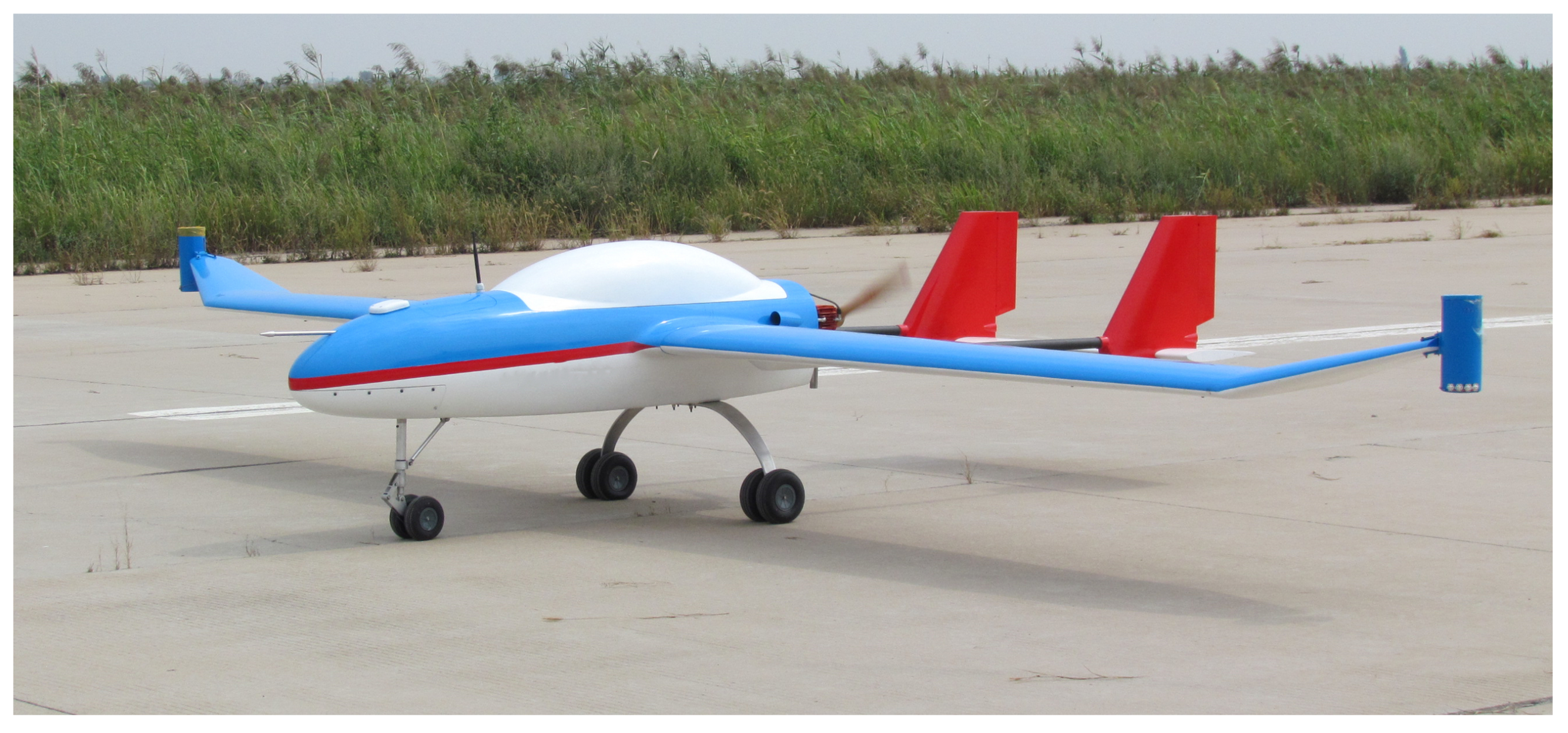
Figure 1. The coordinate systems and convention of fixed-wing aircraft.
Drones 07 00324 g001
Figure 2. The flowchart of automatic landing using modified DWA.
Drones 07 00324 g002
Figure 3. Schematic representation of windows.
Drones 07 00324 g003
Figure 4. An example: motion primitives generated by dynamic window.
Drones 07 00324 g004
Figure 5. Link the current pose to the target pose with the Dubins path when y c 1 > R . The colored lines and arcs represent the heuristic path.
Drones 07 00324 g005
Figure 6. Link the current pose to the target pose by Dubins path when y c 1 R and y c 2 R . The colored lines and arcs represent the heuristic path.
Drones 07 00324 g006
Figure 7. Link the current pose to the target pose with the Dubins path when y c 1 R and y c 2 < R . The colored lines and arcs represent the heuristic path.
Drones 07 00324 g007
Figure 8. The 3 stages in landing of fixed-wing aircraft.
Drones 07 00324 g008
Figure 9. Schematic diagrams of losing altitude (excess gravitational potential energy). (a) 3D view; (b) lateral view.
Drones 07 00324 g009aDrones 07 00324 g009b
Figure 10. The fixed-wing UAV: YuanZheng-6.
Drones 07 00324 g010
Figure 11. The flowchart of numerical simulation.
Drones 07 00324 g011
Figure 12. The time consumed by M-DWA. (a) The time consumed by one iteration; (b) The cumulative time consumed by iterations.
Drones 07 00324 g012
Figure 13. Starting from a point with different initial heading angles and landing on a fixed point. (a) landing path (3D view); (b) landing path (lateral view); (c) landing path (top view); (d) heading angle ψ ; (e) speed V; (f) angular rate ω .
Drones 07 00324 g013
Figure 14. Starting from a point with different initial altitude and landing on a fixed point. (a) landing path (3D view); (b) landing path (lateral view); (c) landing path (top view); (d) heading angle ψ ; (e) speed V; (f) angular rate ω .
Drones 07 00324 g014
Figure 15. Starting from the same point and landing on a moving target point. (a) landing path (3D view); (b) landing path (lateral view); (c) landing path (top view); (d) heading angle ψ ; (e) speed V; (f) angular rate ω .
Drones 07 00324 g015
Table 1. Characteristics and performance of the aircraft.
CharacteristicsRangePerformanceRange
Length3.2 mMax/Loiter Speed38/31 m/s
Wing Span6.4 mStall speed24 m/s
Gross weight90.0 kgMin turning radius96 m
Max thrust35.0 kg
Table 2. Parameters used in the numerical simulation.
ParametersValuesParametersValuesParametersValues
V min / V max 25/34 m/s ω min / ω max π 9 / π 9 rad/s t 0.1 s
a min / a max −2.3/3.5 m/s2 α min / α max π 3 / π 3 rad/s 2 t r 0.2 s
V i 25 m/sResolution of V0.2 m/s λ y 0.5
γ i −0.07 radResolution of ω π 90 rad/s λ V 0.02
R100 m T 0.6 s λ t 8
Disclaimer/Publisher’s Note: The statements, opinions and data contained in all publications are solely those of the individual author(s) and contributor(s) and not of MDPI and/or the editor(s). MDPI and/or the editor(s) disclaim responsibility for any injury to people or property resulting from any ideas, methods, instructions or products referred to in the content.

