
IRelNet: An Improved Relation Network for Few-Shot Radar Emitter Identification

Abstract
:1. Introduction
- The proposed IRelNet model, which can be embedded in UAVs, is presented. This network could substantially improve the performance of the REI techniques in few-shot scenarios.
- IRelNet was augmented with both channel attention and spatial attention, which served to augment its capability to extract the deep features of samples.
- To counteract the vanishing gradient problem and improve the stability of IRelNet, a skip connection was integrated into IRelNet.
- The details of how IRelNet embedded in UAVs was utilized to address the real EW scene are presented.
2. Radar Emitter Signal Preprocessing
2.1. WVD
2.2. Bicubic Interpolation
3. Method
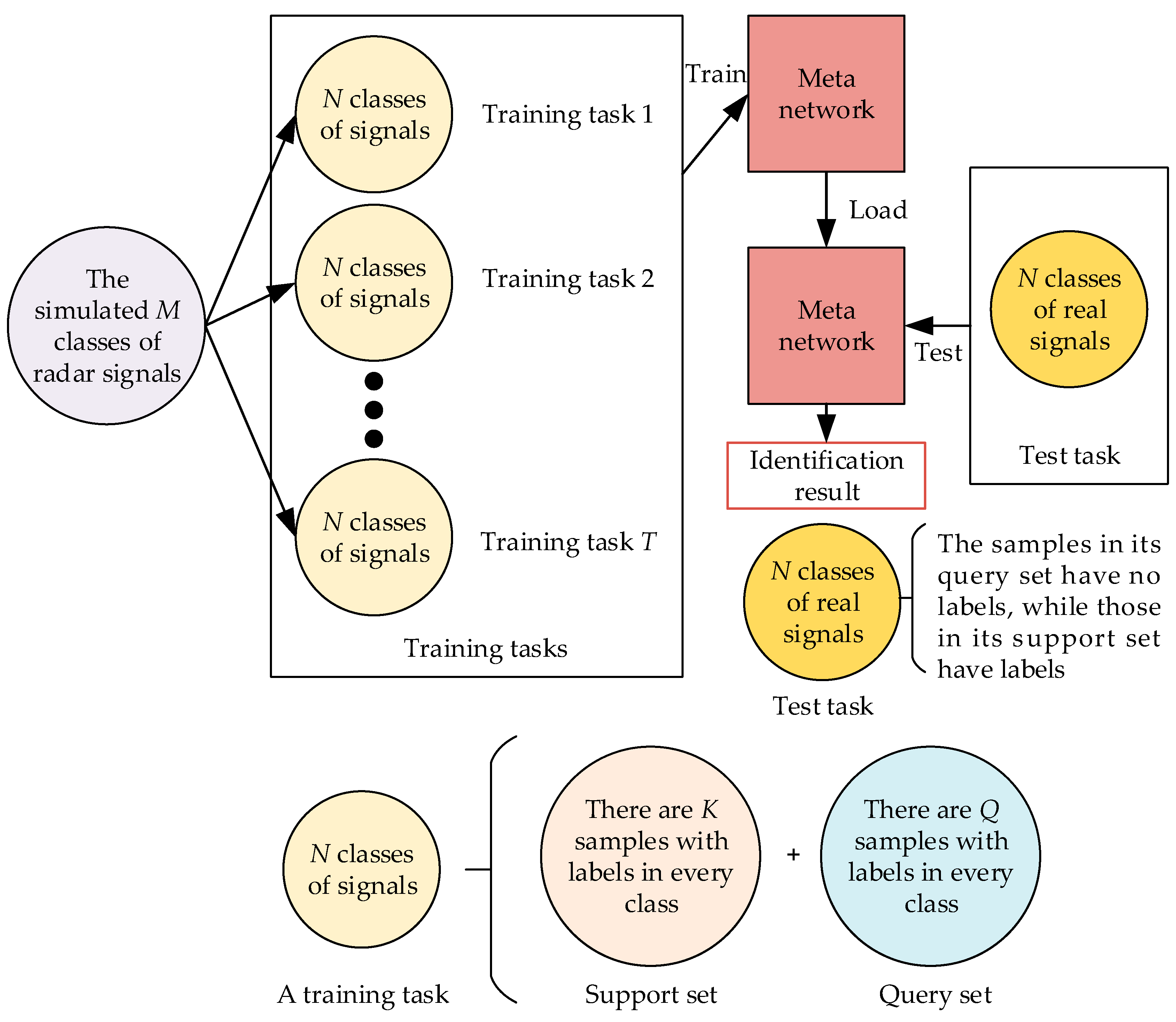
3.1. REI Scene
3.2. REI Algorithm
3.3. IRelNet
4. Experiments
4.1. Datasets
4.2. Model Optimization
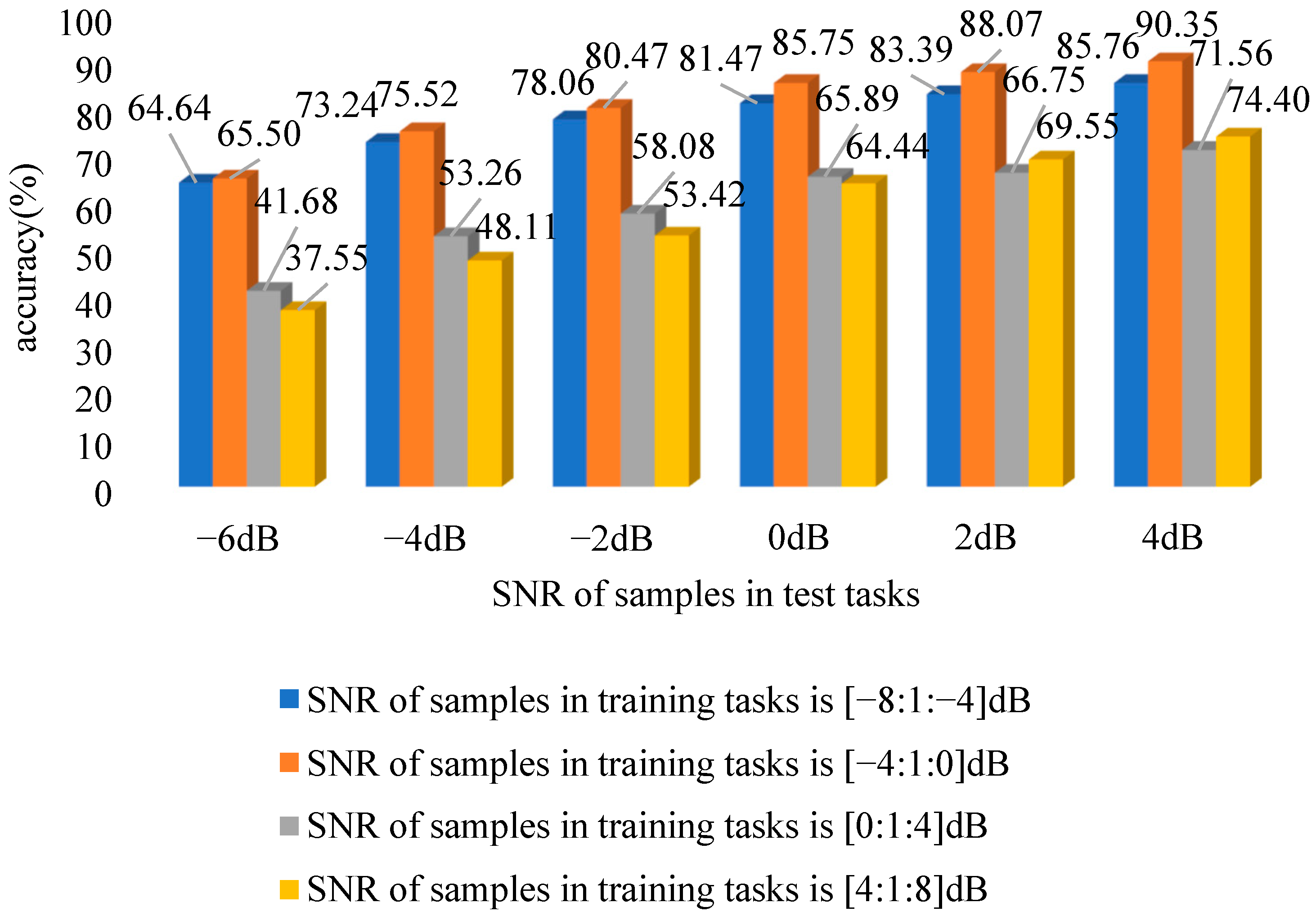
4.3. Influence of SNR
4.4. Influence of Classes N and the Number K
4.5. Performance of Different Methods
5. Conclusions
Author Contributions
Funding
Data Availability Statement
Conflicts of Interest
References
- Sharma, P.; Sarma, K.K.; Mastorakis, N.E. Artificial intelligence aided electronic warfare systems- recent trends and evolving applications. IEEE Access 2020, 8, 224761–224780. [Google Scholar] [CrossRef]
- Wiley, R.G. Electronic Intelligence: The Analysis of Radar Signals, 1st ed.; Artech House: Dedham, MA, USA, 1982. [Google Scholar]
- Wilkinson, D.R.; Watson, A.W. Use of metric techniques in ESM data processing. IEE Proc. F (Commun. Radar Signal Process.) 1985, 132, 229–232. [Google Scholar] [CrossRef]
- Grant, P.M.; Collins, J.H. Introduction to electronic warfare. IEE Proc. F (Commun. Radar Signal Process.) 1982, 129, 113–132. [Google Scholar] [CrossRef]
- Yang, N.; Zhang, B.; Ding, G.; Wei, Y.; Wang, J.; Guo, D. Specific emitter identification with limited samples: A model-agnostic meta-learning approach. IEEE Commun. Lett. 2021, 26, 345–349. [Google Scholar] [CrossRef]
- Al-Emadi, S.; Al-Senaid, F. Drone detection approach based on radio-frequency using convolutional neural network. In Proceedings of the 2020 IEEE International Conference on Informatics, IoT, and Enabling Technologies (ICIoT), Doha, Qatar, 2–5 February 2020. [Google Scholar]
- Nemer, I.; Sheltami, T.; Ahmad, I.; Yasar, A.U.-H.; Abdeen, M.A.R. RF-based UAV detection and identification using hierarchical learning approach. Sensors 2021, 21, 1947. [Google Scholar] [CrossRef] [PubMed]
- Gan, J.; Hu, A.; Kang, Z.; Qu, Z.; Yang, Z.; Yang, R.; Wang, Y.; Shao, H.; Zhou, J. SAS-SEINet: A SNR-Aware Adaptive Scalable SEI Neural Network Accelerator Using Algorithm–Hardware Co-Design for High-Accuracy and Power-Efficient UAV Surveillance. Sensors 2022, 22, 6532. [Google Scholar] [CrossRef]
- Al-Sa’d, M.F.; Al-Ali, A.; Mohamed, A.; Khattab, T.; Erbad, A. RF-Based Drone Detection and Identification Using Deep Learning Approaches: An Initiative towards a Large Open Source Drone Database. Future Gener. Comput. Syst. 2019, 100, 86–97. [Google Scholar] [CrossRef]
- Visnevski, N.; Krishnamurthy, V.; Wang, A.; Haykin, S. Syntactic modeling and signal processing of multifunction radars: A stochastic context-free grammar approach. Proc. IEEE 2007, 95, 1000–1025. [Google Scholar] [CrossRef]
- Visnevski, N.; Haykin, S.; Krishnamurthy, V.; Dilkes, F.A.; Lavoie, P. Hidden Markov models for radar pulse train analysis in electronic warfare. In Proceedings of the IEEE International Conference on Acoustics, Speech, and Signal Processing, Philadelphia, PA, USA, 23 March 2005. [Google Scholar]
- Li, C.; Wang, W.; Wang, X. A method for extracting radar words of multi-function radar at data level. In Proceedings of the IET International Radar Conference 2013, Xi’an, China, 14–16 April 2013. [Google Scholar]
- Matuszewski, J. The analysis of modern radar signals parameters in electronic intelligence system. In Proceedings of the 2016 13th International Conference on Modern Problems of Radio Engineering, Telecommunications and Computer Science (TCSET), Lviv, Ukraine, 23–26 February 2016. [Google Scholar]
- Cai, J.; Li, C.; Zhang, H. Modulation recognition of radar signal based on an improved CNN model. In Proceedings of the 2019 IEEE 7th International Conference on Computer Science and Network Technology (ICCSNT), Dalian, China, 19–20 October 2019. [Google Scholar]
- Wu, J.; Zhong, Y.; Chen, A. Radio modulation classification using STFT spectrogram and CNN. In Proceedings of the 2021 7th International Conference on Computer and Communications (ICCC), Chengdu, China, 10–13 December 2021. [Google Scholar]
- Chen, K.; Zhang, J.; Chen, S.; Zhang, S.; Zhao, H. Automatic modulation classification of radar signals utilizing X-net. Digit. Signal Process. 2022, 123, 103396. [Google Scholar] [CrossRef]
- Hou, C.; Fang, C.; Lin, Y.; Li, Y.; Zhang, J. Implementation of a CNN identifying modulation signals on an embedded SoC. In Proceedings of the 2020 IEEE 63rd International Midwest Symposium on Circuits and Systems (MWSCAS), Springfield, MA, USA, 9–12 August 2020. [Google Scholar]
- Hou, C.; Li, Y.; Chen, X.; Zhang, J. Automatic modulation classification using KELM with joint features of CNN and LBP. Phys. Commun. 2021, 45, 101259. [Google Scholar] [CrossRef]
- Zhang, M.; Diao, M.; Guo, L. Convolutional neural networks for automatic cognitive radio waveform recognition. IEEE Access 2017, 5, 11074–11082. [Google Scholar] [CrossRef]
- Kong, S.H.; Kim, M.; Hoang, L.M.; Kim, E. Automatic LPI radar waveform recognition using CNN. IEEE Access 2018, 6, 4207–4219. [Google Scholar] [CrossRef]
- Qu, Z.; Mao, X.; Deng, Z. Radar signal intra-pulse modulation recognition based on convolutional neural network. IEEE Access 2018, 6, 43874–43884. [Google Scholar] [CrossRef]
- Tian, X.; Sun, X.; Yu, X.; Li, X. Modulation pattern recognition of communication signals based on fractional low-order Choi-Williams distribution and convolutional neural network in impulsive noise environment. In Proceedings of the 2019 IEEE 19th International Conference on Communication Technology (ICCT), Xi’an, China, 16–19 October 2019. [Google Scholar]
- Zhu, M.; Li, Y.; Pan, Z.; Yang, J. Automatic modulation recognition of compound signals using a deep multi-label classifier: A case study with radar jamming signals. Signal Process. 2020, 169, 107393. [Google Scholar] [CrossRef]
- Sun, W.; Wang, L.; Sun, S. Radar emitter individual identification based on convolutional neural network learning. Math. Probl. Eng. 2021, 2021, 5341940. [Google Scholar] [CrossRef]
- Peng, L.; Qu, W.; Zhao, Y.; Wu, Y. A multi-level network for radio signal modulation classification. In Proceedings of the International Conference on Artificial Intelligence, Information Processing and Cloud Computing, Sanya, China, 19 December 2019. [Google Scholar]
- Shao, G.; Chen, Y.; Wei, Y. Convolutional neural network-based radar jamming signal classification with sufficient and limited samples. IEEE Access 2020, 8, 80588–80598. [Google Scholar] [CrossRef]
- O’Shea, T.J.; West, N.; Vondal, M.; Clancy, T.C. Semi-supervised radio signal identification. In Proceedings of the 2017 19th International Conference on Advanced Communication Technology (ICACT), Pyeongchang-gun, Republic of Korea, 19–22 February 2017. [Google Scholar]
- Hospedales, T.; Antoniou, A.; Micaelli, P.; Storkey, A. Meta-Learning in neural networks: A survey. IEEE Trans. Pattern Anal. Mach. Intell. 2022, 44, 5149–5169. [Google Scholar] [CrossRef]
- Vanschoren, J. Meta-learning: A survey. arXiv 2018, arXiv:1810.03548. [Google Scholar]
- Li, P. Research on radar signal recognition based on automatic machine learning. Neural Comput. Appl. 2020, 32, 1959–1969. [Google Scholar] [CrossRef]
- Finn, C.B. Learning to Learn with Gradients. Ph.D. Dissertation, Department Computer Science, University of California, Berkeley, CA, USA, 2018. [Google Scholar]
- Bromley, J.; Guyon, I.; LeCun, Y.; Säckinger, E.; Shah, R. Signature verification using a “Siamese” time delay neural network. In Proceedings of the 6th International Conference on Neural Information Processing Systems, Denver, CO, USA, 29 November 1993. [Google Scholar]
- Zagoruyko, S.; Komodakis, N. Learning to compare image patches via convolutional neural networks. In Proceedings of the IEEE Conference on Computer Vision and Pattern Recognition, Boston, MA, USA, 7–12 June 2015. [Google Scholar]
- Vinyals, O.; Blundell, C.; Lillicrap, T.; Kavukcuoglu, K.; Wierstra, D. Matching networks for one shot learning. In Proceedings of the 30th International Conference on Neural Information Processing Systems, Barcelona, Spain, 5 December 2016. [Google Scholar]
- Snell, J.; Swersky, K.; Zemel, R. Prototypical networks for few-shot learning. In Proceedings of the part of Advances in Neural Information Processing Systems 30, Long Beach, CA, USA, 4–9 December 2017. [Google Scholar]
- Sung, F.; Yang, Y.; Zhang, L.; Xiang, T.; Torr, P.H.S.; Hospedales, T.M. Learning to compare: Relation network for few-shot learning. In Proceedings of the 2018 IEEE/CVF Conference on Computer Vision and Pattern Recognition, Salt Lake City, UT, USA, 18–23 June 2018. [Google Scholar]
- Nair, V.; Hinton, G.E. Rectified linear units improve restricted Boltzmann machines. In Proceedings of the International Conference on Machine Learning, Haifa, Israel, 21–24 June 2010. [Google Scholar]
- Huang, J.; Wu, B.; Li, P.; Li, X.; Wang, J. Few-shot learning for radar emitter signal recognition based on improved prototypical network. Remote Sens. 2022, 14, 1681. [Google Scholar] [CrossRef]
- Lang, P.; Fu, X.; Martorella, M.; Dong, J.; Qin, R.; Feng, C.; Zhao, C. RRSARNet: A novel network for radar radio sources adaptive recognition. IEEE Trans. Veh. Technol. 2021, 70, 11483–11498. [Google Scholar] [CrossRef]
- Zhang, Z.; Li, Y.; Zhai, Q.; Li, Y.; Gao, M. Few-shot learning for fine-grained signal modulation recognition based on foreground segmentation. IEEE Trans. Veh. Technol. 2022, 71, 2281–2292. [Google Scholar] [CrossRef]
- Sun, G. RF Transmitter identification using combined Siamese networks. IEEE Tran. Instrum. Meas. 2022, 71, 8000813. [Google Scholar] [CrossRef]
- Dong, Y.; Jiang, X.; Zhou, H.; Lin, Y.; Shi, Q. SR2CNN: Zero-shot learning for signal recognition. IEEE Trans. Signal Process. 2021, 69, 2316–2329. [Google Scholar] [CrossRef]
- Xu, H.; Wang, J.; Li, H.; Ouyang, D.; Shao, J. Unsupervised meta-learning for few-shot learning. Pattern Recognit. 2021, 116, 107951. [Google Scholar] [CrossRef]
- Gong, J.; Xu, X.; Lei, Y. Unsupervised specific emitter identification method using radio-frequency fingerprint embedded InfoGAN. IEEE Trans. Inf. Forensics Secur. 2020, 15, 2898–2913. [Google Scholar] [CrossRef]
- Cao, R.; Cao, J.; Mei, J.P.; Yin, C.; Huang, X. Radar emitter identification with bispectrum and hierarchical extreme learning machine. Multimed. Tools Appl. 2019, 78, 28953–28970. [Google Scholar] [CrossRef]
- Yan, X.; Liu, G.; Wu, H.C.; Zhang, G.; Wang, Q.; Wu, Y. Robust modulation classification over α-stable noise using graph-based fractional lower-order cyclic spectrum analysis. IEEE Trans. Veh. Technol. 2020, 69, 2836–2849. [Google Scholar] [CrossRef]
- Yan, X.; Liu, G.; Wu, H.C.; Feng, G. New automatic modulation classifier using cyclic-spectrum graphs with optimal training features. IEEE Commun. Lett. 2018, 22, 1204–1207. [Google Scholar] [CrossRef]
- Sun, L.; Wang, X.; Huang, Z.; Li, B. Radio frequency fingerprint extraction based on feature inhomogeneity. IEEE Internet Things J. 2022, 9, 17292–17308. [Google Scholar] [CrossRef]
- Keys, R. Cubic convolution interpolation for digital image processing. IEEE Trans. Acoust. Speech Signal Process. 1981, 29, 1153–1160. [Google Scholar] [CrossRef]
- Liu, M.; Liao, G.; Zhao, N.; Song, H.; Gong, F. Data-driven deep learning for signal classification in industrial cognitive radio networks. IEEE Trans. Ind. Inform. 2021, 17, 3412–3421. [Google Scholar] [CrossRef]


| Step | Details |
|---|---|
| Step 1 | The desired size of the initial is set to , and the matrix obtained via bicubic interpolation is represented as ; |
| Step 2 | According to the size of and , the scaling factor is calculated via and , where and represent the sizes of rows and columns of a matrix, respectively; |
| Step 3 | The bicubic interpolation function, , is expressed as ; |
| Step 4 | (1) Every element is obtained from the desired matrix , where and represent the row and the column, respectively, of the element in ; (2) The position in the initial corresponding to the position is calculated using ; (3) Sixteen elements closest to the position in , where and represents the row and column, respectively, of the element in , are obtained; (4) According to the formula, , is obtained; |
| Step 5 | The process of executing bicubic interpolation on an initial discrete WVD is performed, and the matrix with the desired size is obtained. |
| Class | Parameters |
|---|---|
| LFM | Frequency bandwidth ∈ [15, 20] MHz; carrier frequency ∈ [25, 30] MHz |
| NLFM | Frequency bandwidth ∈ [10, 15] MHz; carrier frequency ∈ [25, 30] MHz |
| CW | carrier frequency∈ [25, 30] MHz |
| FD | Frequency F1 ∈ [5, 10] MHz; frequency F2 ∈ [15, 20] MHz; frequency F3 ∈ [25, 30] MHz |
| BPSK | Phase coding sequence [1, 1, 1, 0, 0, 1, 0]; carrier frequency ∈ [25, 30] MHz |
| BFSK | Frequency coding sequence [1, 1, 0, 0, 0, 1, 0, 0, 1]; frequency F1 ∈ [10, 15] MHz; frequency F2 ∈ [25, 30] MHz |
| BASK | Amplitude coding sequence [1, 1, 1, 0, 1, 0, 0, 1, 0, 0]; carrier frequency ∈ [25, 30] MHz |
| Baker-LFM | Barker coding sequence [1, 1, 1, 0, 0, 0, 0, 1, 0, 1, 0]; frequency bandwidth ∈ [10, 15] MHz; carrier frequency ∈ [25, 30] MHz |
| All signals have a PW of 10 μs and a sampling rate of 100 MHz | |
| Configurations | −6 dB | −4 dB | −2 dB | 0 dB | 2 dB | 4 dB | |
|---|---|---|---|---|---|---|---|
| T = 500 | B = 3 | 0.6521 | 0.6772 | 0.7171 | 0.7541 | 0.7850 | 0.8152 |
| T = 1000 | B = 3 | 0.7433 | 0.7246 | 0.7372 | 0.7703 | 0.7903 | 0.7979 |
| T = 1500 | B = 3 | 0.5628 | 0.5892 | 0.6935 | 0.7294 | 0.7847 | 0.7812 |
| T = 500 | B = 4 | 0.5634 | 0.7028 | 0.7806 | 0.7980 | 0.8568 | 0.8685 |
| T = 1000 | B = 4 | 0.6550 | 0.7552 | 0.8047 | 0.8575 | 0.8807 | 0.9035 |
| T = 1500 | B = 4 | 0.5974 | 0.7206 | 0.8001 | 0.8322 | 0.8776 | 0.8768 |
| T = 500 | B = 5 | 0.4332 | 0.5238 | 0.5233 | 0.5643 | 0.5622 | 0.5795 |
| T = 1000 | B = 5 | 0.5736 | 0.6806 | 0.7135 | 0.7591 | 0.7870 | 0.8006 |
| T = 1500 | B = 5 | 0.6313 | 0.6678 | 0.7352 | 0.7670 | 0.7707 | 0.7687 |
| Test Tasks | 0 dB, 1 dB, 2 dB | −2 dB, −1 dB, 0 dB | −4 dB, −3 dB, −2 dB | |
|---|---|---|---|---|
| Training Tasks | ||||
| 0 dB, 1 dB, 2 dB | 66.53 | 64.85 | 62.42 | |
| −2 dB, −1 dB, 0 dB | 76.80 | 73.75 | 75.12 | |
| −4 dB, −3 dB, −2 dB | 55.75 | 53.77 | 43.19 | |
| Method | PN | RN | RRSARNet | IRelNet |
|---|---|---|---|---|
| Time | 1.5280 s | 2.6440 s | 3.5430 s | 5.9160 s |
Disclaimer/Publisher’s Note: The statements, opinions and data contained in all publications are solely those of the individual author(s) and contributor(s) and not of MDPI and/or the editor(s). MDPI and/or the editor(s) disclaim responsibility for any injury to people or property resulting from any ideas, methods, instructions or products referred to in the content. |
© 2023 by the authors. Licensee MDPI, Basel, Switzerland. This article is an open access article distributed under the terms and conditions of the Creative Commons Attribution (CC BY) license (https://creativecommons.org/licenses/by/4.0/).
Share and Cite
Wu, Z.; Du, M.; Bi, D.; Pan, J. IRelNet: An Improved Relation Network for Few-Shot Radar Emitter Identification. Drones 2023, 7, 312. https://doi.org/10.3390/drones7050312
Wu Z, Du M, Bi D, Pan J. IRelNet: An Improved Relation Network for Few-Shot Radar Emitter Identification. Drones. 2023; 7(5):312. https://doi.org/10.3390/drones7050312
Chicago/Turabian StyleWu, Zilong, Meng Du, Daping Bi, and Jifei Pan. 2023. "IRelNet: An Improved Relation Network for Few-Shot Radar Emitter Identification" Drones 7, no. 5: 312. https://doi.org/10.3390/drones7050312