Article

On Countermeasures against Cooperative Fly of UAV Swarms

Information System Engineering College, Strategic Support Force Information Engineering University, Zhengzhou 450001, China
*
Author to whom correspondence should be addressed.
Drones 2023, 7(3), 172; https://doi.org/10.3390/drones7030172
Submission received: 1 December 2022 / Revised: 26 February 2023 / Accepted: 27 February 2023 / Published: 2 March 2023
(This article belongs to the Special Issue Wireless Networks and UAV)

Abstract

:
Aiming at anti Unmanned Aerial Vehicle (UAV) swarm, this paper studies the detection and suppression mechanisms of emergence in cooperative flight. Cooperative fly is one of the critical operations for UAV swarm in both military and civilian utilities, which allows individual UAVs to distributed adjust their velocity to head for a common destination as well as avoid a collision. This process is viewed as the emergence of complex systems. An emergence detection algorithm based on double thresholds is proposed. It simultaneously monitors the cooperative flight process and system connectivity to accurately identify the occurrence, achievement, or failure of cooperative fly, which provides a solid prerequisite for the suppression mechanism. For suppression, in-band radio interference is designed under the constraint of average power, and the effect is modeled from the perspective of degrading the communication performance of the target system. It is found that low-intensity continuous interference can effectively delay the cooperative fly process and has better concealment, while medium-intensity continuous interference can rapidly stop that process. Based on the above analysis, for the first time, two countermeasures for the UAV swarm’s cooperative fly are designed for the operation intent of delay and disruption of the target UAC swarms, respectively. Simulation results show the effectiveness of the countermeasures.

1. Introduction

As one of the revolutionary forces of the future battlefield, UAV swarms have significant potential in surveillance reconnaissance, electronic countermeasures, and cooperative penetration. Compared with traditional means, UAV swarms have several advantages, including a high cost-efficiency ratio, intelligence information gathering, and improved systematic survivability [1,2]. Due to the promotion of projects such as Grey Partridge [3] and Gremlins [4,5], the key technologies of UAV swarms have become more mature, and the UAV swarms have begun to emerge in many combat operations.
To deal with the potential threat of UAV swarms in modern battlefields, countries actively promote the research and development of countermeasures against it. Transmitting RF signals to destroy the target UAV system is a typical method of an anti-UAV swarm, divided into hard kill and soft kill according to the damage degree. Hard kill refers to using high-power RF signals to damage target systems, especially communication-related devices. In ref. [6], the authors studied the damage of broadband high-power electromagnetic pulse to the UAV components based on the quadrotor UAV and pointed out that the receiver and GPS are the most vulnerable modules. Moreover, in ref. [7], the authors established a nonlinear interference model for this problem and discussed the influence of pulse width and repetition frequency on the interference effect given average/peak interference power. Besides, in ref. [8] the authors analyzed the interference effect of an HPRF ultra-wide spectrum electromagnetic pulse jammer on the GPS module of a micro-UAV through experiments. Soft kill mainly includes deceiving the target system by transmitting false navigation or interfering with normal communication. Compared with a hard kill, it does not necessarily damage the UAV entity but can seriously interfere with the target’s tasks and does not require high-power equipment. The interference behavior is more intelligent and hidden, so it has a broad application prospect.
However, the countermeasures against a single UAV are unsuitable for the UAV swarms. Some researchers proposed to consider the UAV swarms as a whole system and designed countermeasures from the perspective of destroying the UAV’s network topology and system state [9,10,11]. In UAV swarms, individual UAVs often need to achieve cooperative flight, as all UAVs have the same speed direction and similar speed while avoiding collisions [12]. Before the cooperative fly is achieved, the system is in a disordered state and vulnerable. While, when a cooperative flight is achieved, the system becomes more robust to malicious attacks. It can be found that the process is a relatively fragile stage of the system, which is a rare opportunity for the counterpart. To achieve cooperative flight, information interaction is required in the UAV swarm, typically accomplished by wireless communication. Due to the broadcast nature of wireless media, this process is vulnerable to RF interference [13,14]. Thus, refs. [15,16] proposed countermeasures to destroy the UAV swarm cooperative flight. These works viewed “swarm” cooperative flight as a complex system with emergent characteristics and established a “swarm” emergent measurement model based on f-divergence [17], where judging the swarm control failure under interference was established for the first time. Experiments analyzed the influence of the interference intensity and the interference opportunity on the behavior of suppressing the cooperative fly of a UAV swarm.
This work provides a valuable reference for this paper. However, the following problems exist. First, existing research lacks the support of a cluster motion model, which plays a crucial role in the emergence detection algorithm. Second, existing algorithms focus on emergence evaluation under a given attribute of the target system. However, research on which attribute(s) to adopt and how to use multiple attributes comprehensively are rarely considered. Third, there is little analysis of the effectiveness of suppression mechanisms in complex confrontations, such as on battlefields. For example, if the counterparty increases the interference signal strength, it may be detected by the target system and fail. Therefore, it is necessary to design and evaluate the counterattack behavior by considering reducing the probability of being detected.
Aiming at the above problems, the main contributions of this paper are as follows: ① based on the classic cooperative fly model, a dual threshold detection algorithm is proposed. The recognition accuracy is improved through joint detection velocity and network connectivity, which provides a basis for countermeasures. ② the suppression behavior is modeled, and comprehensive comparisons are carried out with different duty cycles/interference signal strength/interference patterns, which makes a primary reference for the design of counterattack mechanisms. ③ The countermeasures are designed according to different operational intentions, and their effectiveness is illustrated by simulation.
For the convenience of description, the basic assumptions of this paper are given. Assume that the UAV swarm contains 100 nodes [15,16], which are released by the host at the 0th second and the cooperative fly is started at the 11th second. Each UAV has a set of wireless transceivers with a communication radius of R meters. Due to the small number of communication barriers, short distance, and low relative speed between UAVs, the wireless channel between UAVs is assumed to be an Additive White Gaussian Noise (AWGN) channel, and the unilateral power spectral density of the noise is n0 [17]. The bandwidth is B Hz, and because the flying heights of the individuals in the UAV swarm are similar, only the position on the 2D plane is considered. In this paper, the UAV is assumed to be a mobile particle within a 2-D plane, the influence of its mechanical characteristics on motion and motion in the 3-D space will be left for follow-up study.

2. Cooperative Fly Detection for UAV Swarm

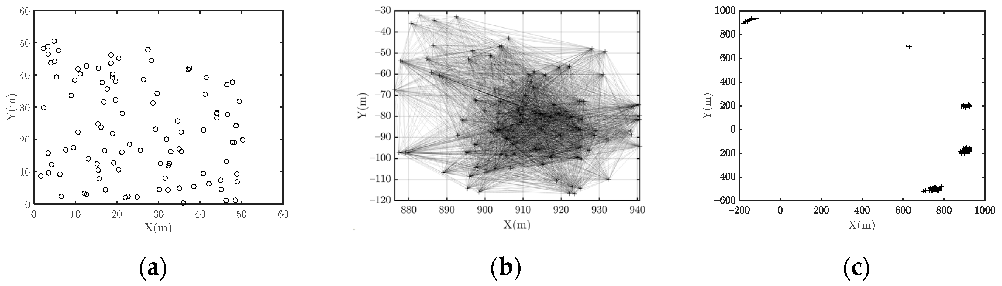
2.1. UAV Swarm Cluster Motion Model

Several cluster motion models have been proposed in the literature, among which the Vicsek Model (VM) is one of the most famous models [18]. It is assumed that there are N nodes in the system, known as V = { i | 1 = 1 , , N } . When released by the host plane, the UAVs are set with the same speed (noted as v0), random directions, and positions. At tth second, the position of node i is known as X i ( t ) , and the direction is known as θ i ( t ) , where θ i ( t ) is uniformly distributed over [ π , π ), and the velocity is denoted as V i ( t ) = [ v 0 c o s θ i ( t ) , v 0 s i n θ i ( t ) ] . Then, the position of node i at moment t + 1 is updated as follows:
X i ( t + 1 ) = X i ( t ) + V i ( t )
In the VM model, the node adjusts its direction to the mean value of the other neighboring nodes. Nevertheless, there exists a random error due to inaccurate observation, known as ξ i ( t ) , which is assumed to obey the Gaussian distribution with a mean value of 0:
θ i ( t + 1 ) = θ i ( t ) Γ i ( t ) + ξ i ( t )
where . Γ means averaging within the set Γ , Γ i ( t ) is the node set centered at i with radius R, and R is the synchronization radius, which in this situation is the wireless communication radius.
Γ i ( t ) = { j | X j ( t ) X i ( t ) R , j V , j i }
It is shown that all nodes have the same velocity if the UAV swarm is connected. If at t s u c , for any node i and j, the following formula holds:
| θ i ( t s u c ) θ j ( t s u c ) | ε
The system is considered to reach perfect cooperative flight. In Formula (4), ε describes the acceptable error range. T s u c is the duration between the start time and t s u c and it is known as synchronous time.

2.2. Cooperative Fly Detection of UAV Swarm

2.2.1. Analysis of Existing Algorithms

Detecting the cooperative fly is the premise for suppressing it. Existing methods focus on quantitative description of emergence intensity, with typical methods being:
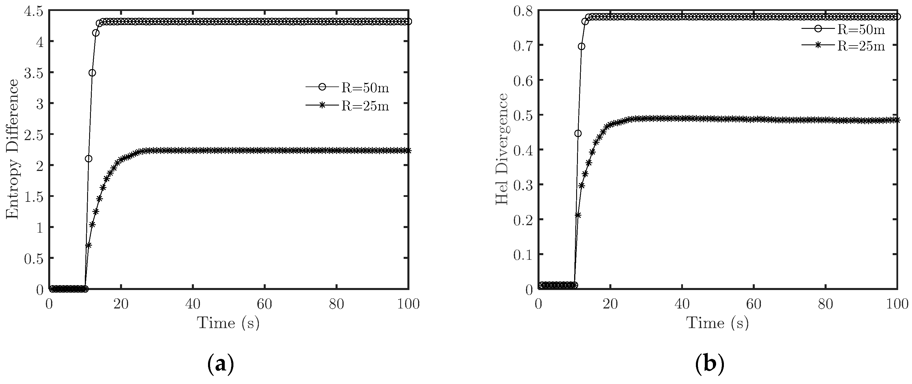
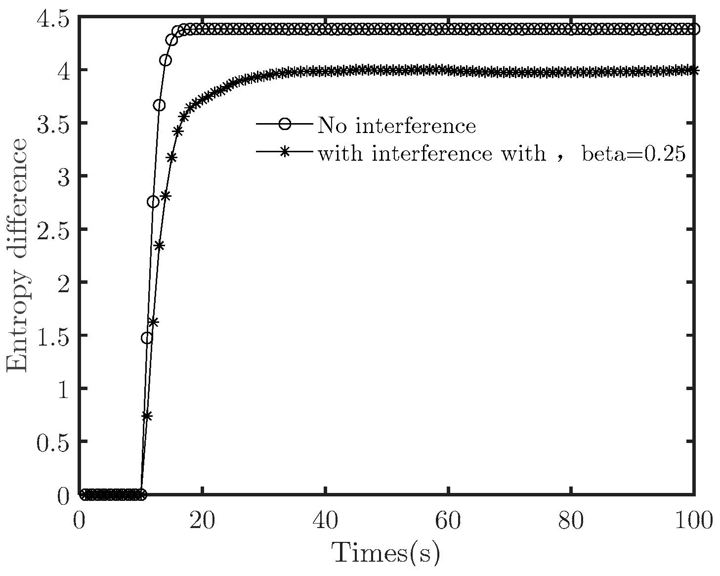
  • Entropy-difference-based method [19]
The system’s attribute is taken as a random variable, and its PDF (Probability Distribution Function) is evaluated by a Parzen window. Based on the PDF, the entropy at t is calculated as the following
H t = i = 1 K p i ( t ) l o g 2 ( 1 p i ( t ) )
where p i ( t ) is the discrete probability of the attribute at t, and K is the number of values.
Moreover, the difference between entropy at t and 0 is used to measure the emergence intensity:
E = H t H 0
If E > 0 , it suggests that emergence starts. The value of E increases with time, and when its increase slows down and E reaches a stable value, a cooperative flight is achieved.
2.
Diversity-based method
Diversity is a measurement for the difference between two probability distributions, for example, KL diversity and f-diversity. Qu et al. [20] compared various measures from the perspective of measurability, convergence, and sensibility and concluded that Hel-divergence is the best measure. The Hel diversity is defined as follows:
D H e l ( P ( x ) | Q ( x ) ) = 1 i = 1 N p i q i
where P ( x )   and   Q ( x ) is the PDF of a random variable X at times t 1   and   t 2 , respectively. The key to calculating the Hel diversity is evaluating the PDF. Given X = { x i } . i = 1 , , N as the samples, the PDF is evaluated as follows [20]:
p ( x ) = 1 N h i = 1 , , N K ( x x i h )
where h is the window width and K(t) is the core function expressed as a Gauss function [21]:
K ( t ) = 1 2 π e x p ( t 2 2 )
The Hel diversity between the t0 and t is calculated in the diversity-based method. If D H e l exceeds a threshold, the emergence starts, while if the Hel curve reaches its optimum value, the emergence is achieved.
Nevertheless, a single attribute is not adequate to detect the cooperative fly of a UAV swarm. We will illustrate this with the following experiments.
Let a system comprising 100 UAVs start its flight. The leader sets the UAVs off at the 0th second and starts cooperative fly at the 11th second. We evaluate whether the abovementioned methods can successfully detect the emergence. The experiments are performed when the synchronization radius R is set to 50 and 25 m, and the results are illustrated in Figure 1.
As presented in Figure 1a, the curves have a similar trend when R is set to 50 and 25 m, i.e., the entropy difference increases first and then stabilizes. The experiment on Hel diversity (as shown in Figure 1b) is similar to Figure 1a. However, if we inspect the network connectivity, we find the differences between the two cases. When the simulations start, the networks are connected, and the nodes are distributed in the 50 m × 50 m area. The topology is depicted in Figure 2a. When R = 50 m, at the end of the simulations, the network is still connected, and the nodes are distributed in a larger area (Figure 2b). When R = 25 m, the network splits into multiple disconnected sub-clusters (Figure 2c). This indicates that when R = 50 m, the system has achieved cooperative fly, but when R = 25 m, at the end of the simulation, the network splits into several disconnected parts. Thus, when R = 25 m, the UAV swarm fails to achieve cooperative flight.

2.2.2. Detection Algorithm of Cooperative Fly of the UAV Swarm Based on Double Thresholds

Due to the lack of a monitor of the system’s connectivity, the existing algorithms cannot accurately determine the achievement of cooperative fly. As a result, the counterpart cannot effectively control the timing for its suppression mechanisms. Aiming at this shortcoming, this paper proposes a detection algorithm based on a double threshold scheme.
The UAV swarm is regarded as a graph G = ( V ,   ) , in which V is the UAV set, the number of V is denoted as N, is the set of communication links between nodes, and the communication links are assumed to be undirected. The connection component N C is defined as a node set where for any node pair i , j N C , there exists at least one path from i to j . Let N c denote the number of nodes in N C . At t, the cluster may split into several disconnected components N C ( k ) ( t ) . Let N C ( k ) ( t ) denote the number of nodes in N C ( k ) ( t ) .
k N C ( k ) ( t ) = V
N C ( k ) ( t ) N C ( m ) ( t ) =
Let connectivity C ( t ) be the ratio of the number of nodes in the maximum connected component [22] to N:
C ( t ) = m a x k { N C ( k ) ( t ) } N
When the UAV swarm is detected, we monitor the node’s velocity and system connectivity, calculate the velocity’s entropy and define the time at which the entropy difference between t and 0 exceeds zero be the emergence start. The increased speed of entropy difference decreases as the emergence is achieved. At the same time, we monitor C ( t ) . If C ( t ) < 1 δ c , then the cooperative fly is destroyed, where δ c is a predefined threshold that reflects the disconnection tolerance. Algorithm 1 is designed as follows.
Algorithm 1. Detection of the Cooperative Fly Emergence based on a Double Threshold
  ① Set the initial parameter value to Φ = { ϕ } ,   L = { l 0 } , δ c
  ② Monitor whether the target UAV swarm appears. If the target UAV swarm is
detected, measure the velocity angles of the individual UAV Φ = { φ i , i = 1 , , N } . Set t = 0,
evaluate the PDF of Φ according to Formula (8), and calculate H0 according to
Formula (5), that is H t = i = 1 K p i ( t ) l o g 2 ( 1 p i ( t ) ) .
  ③ At t, measure the velocity angles of the individual UAV Φ = { φ i , i = 1 , , N } ,
evaluate its PDF according to Formula (8), and calculate the entropy difference
E t = H 0 H t . If E t > 0 , record t as the emergence start time t s t a r t = t , record E t s t a r t , and go
to step ④. Otherwise, go to step ③.
  ④ Set the slide window k to 2, monitor the target system, and record the following state parameters:
   For   t   t = t 0 : t 0 + k
  a. measure the nodes’ velocity angles Φ and evaluate its PDF according to Formula (6),
calculate H t and E t , evaluate the nodes’ position L = { l i , i = 1 , , N } and
calculate C ( t ) according to Formula (10).
  If C ( t ) < 1 δ c , record t as t e n d and go to step ⑤. Otherwise, go to step b and
calculate the three successive entropy differences E t 0 and E t 0 + 1 .
  b. If Δ E 1 = E t 0 + 1 E t 0 > 0   and   Δ E 2 = E t 0 + 2 E t 0 + 1 > 0 , then the cooperative fly
emergence is achieved, and the inference terminates. Record t e n d = i }.
  ⑤ Record the detection result and t = t e n d t s t a r t .

3. Suppression Algorithm of Cooperative Fly for Anti-UAV Swarm

Aiming to suppress the UAV swarm cooperative fly process, an in-band RF signal is released to interfere with the information interaction between UAVs. A question arising is, “How to design interference behavior to be more effective?”. The current work focused on the research of typical communication systems on the increased bit error rate and decreased communication capacity caused by interference [23,24]. However, the influence of the interference behavior on the system state is rarely involved. Thus, this section establishes the RF interference pattern model and compares the effectiveness of different interference behaviors through simulation to provide a basis for the design of countermeasures. Assume that the wireless communication radius is 60 m. The connectivity of the system is required to be no less than 85%, that is, δ c is set to 0.15.

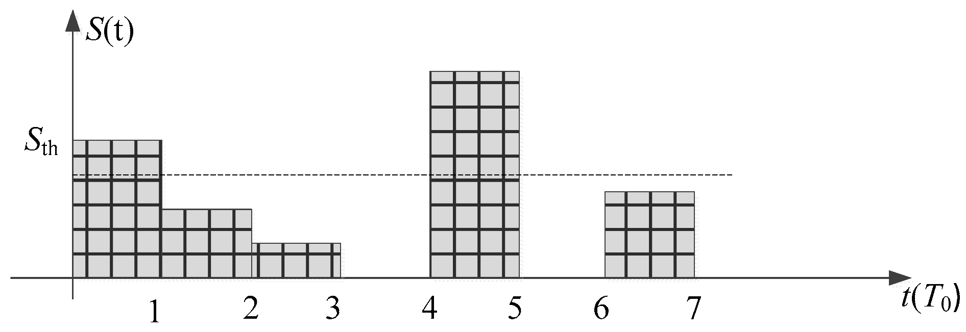
3.1. RF Interference Behavior Modeling

Let the basic pulse be s 0 ( t ) , which has an average unit power, and the duration is T 0 :
s 0 ( t ) = { g ( t ) , 0 t T 0 0 , e l s e
The suppression signal is a sequence comprising delayed and amplified primary pulses:
s I ( t ) = i = 1 M a i d i S i s 0 ( t i T 0 )
where M is the number of primary pulses, ai is whether to emit the pulse at moment i, and a i = 1 means the emission of the pulse and vice versa. di is the duty cycle with 0 d i 1 and S i is the interference power.
Generally, the stronger the power of the jamming signal is, the larger the destruction to the target system is. However, under the confrontation condition, the target system will monitor whether there exists an interference signal. Once interference behavior is detected, the operating frequency will be switched, or the frequency hopping pattern will be changed, leading to interference failure. Therefore, the jamming signal strength cannot be increased blindly, and the jamming scheme should be designed under the strength constraint.
Suppose the target UAV swarm monitors the power of the possible interference signal in its working band. To avoid being detected, the interference signal should satisfy the following constraint:
i = 1 M a i d i 2 S i M S t h
where S t h is the power threshold.
Let I = [ a 1 d 1 2 S 1 , , a M d M 2 S M ] denote the interference pattern, which is typically illustrated in Figure 3 below.
According to Shannon’s formula, the channel capacity of the target UAV system is reduced by the in-band interference signal, that is,
C = B l o g 2 ( 1 + S n 0 B + P I )
Let P I = β n 0 B , where β is called the equivalent noise coefficient. It reflects the extent to which the communication capacity of the UAV swarm is reduced due to interference behavior. Substitute β into Equation (16),
C = B l o g 2 ( 1 + S ( 1 + β ) n 0 B )

3.2. Effectiveness Analysis of Suppression Behavior

In this section, studies on the effectiveness of jamming behavior under typical jamming patterns are carried out through simulations. Because the effect of measuring cooperative fly emergence intensity by entropy difference and Hel divergence is similar, entropy difference is used as the measurement of emergency intensity hereafter.

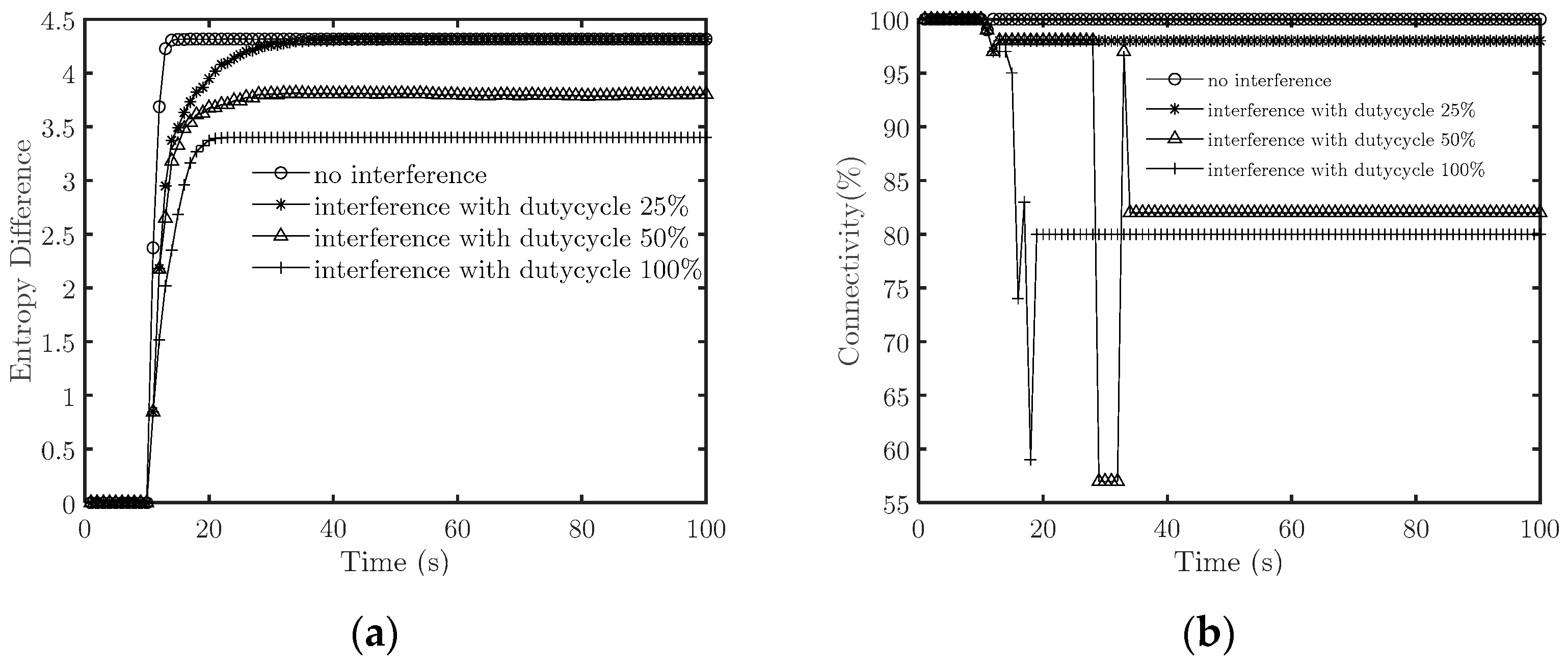
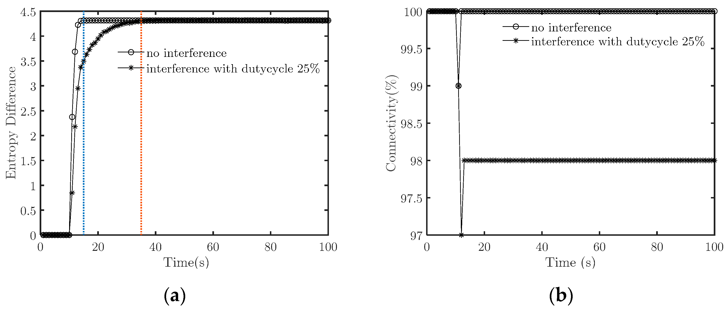
3.2.1. Effectiveness of Suppression Behavior with Equal Intensity and Different Duty Cycles

First, we set β to 1 when the duty cycle is 100%. The interference signal reduces the signal-to-noise ratio to half the original. Figure 4 illustrates how the target system’s entropy differences and connectivity change with time when the duty cycle is 0 (i.e., no interference), 25%, 50%, and 100%.
When there is no interference signal, the entropy difference becomes stable before t = 15 s, and the connectivity remains greater than 95%, so T s u c = 5 s. When emitting an interference signal, the entropy difference first increases with time and then tends to be a constant value. Combined with Figure 5, we find that the system does not achieve cooperative fly when the duty cycle is 100% and 50%, which means the countermeasures succeed. In comparison, the system achieves cooperative flight when the duty cycle is 25%, which means the countermeasures fail. Specifically, when the duty cycle is 50%, the system’s connectivity decreases to about 56%. When t = 29 s, it fluctuates violently and finally stabilizes at about 82%. When the duty cycle is 100%, the interference causes the connectivity to drop to about 75% when t = 17 s, which means the system splits earlier under an interference signal with a large duty cycle.
We further compare the simulation results when there is no interference signal and interference with a 25% duty cycle. Figure 5 highlights that when there is no interference, T s u c = 5 and when the duty cycle is 25%, T s u c = 25 . This reveals that the suppression behavior with a small duty cycle prolongs the synchronization duration by nearly five times. Although this does not prevent the target system from achieving cooperative fly, suppression with low-duty cycles substantially prolongs the process.

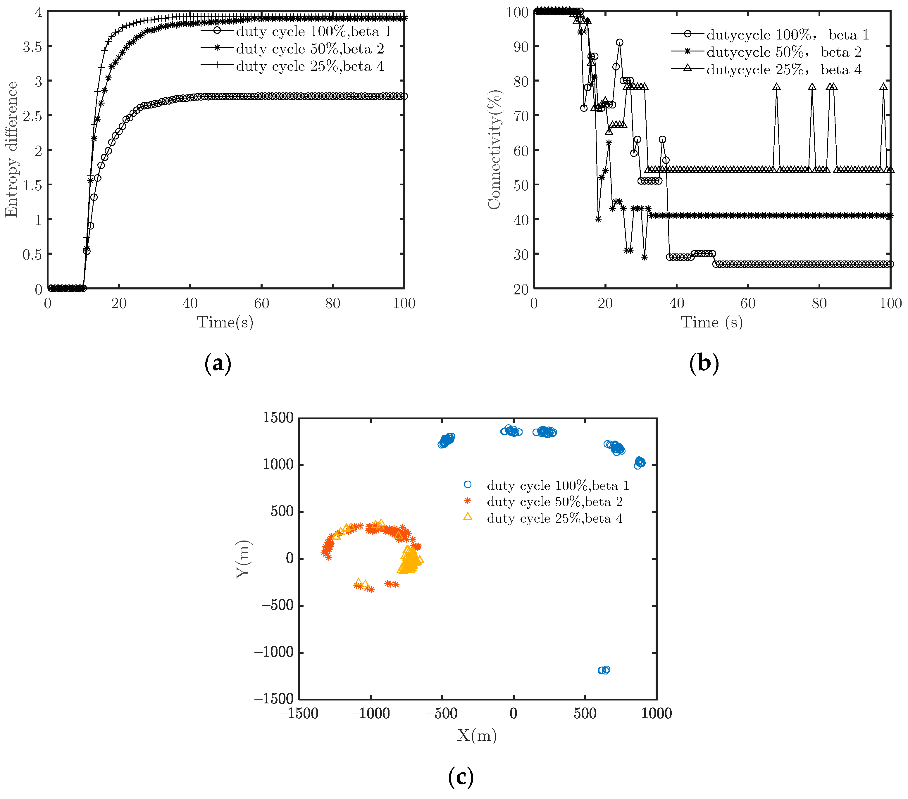
3.2.2. Effectiveness with Equal Average Signal Strength and Different Duty Cycles

Next, we compare the effectiveness between continuous low-intensity and intermittent high-intensity interference signals. To obtain an equal average signal strength, the product of S i and d i is fixed to 1. The simulation parameters are set as follows: ① β = 1 and d i = 100%, ② β = 2 and β = 50%, ③ β = 4 and d i = 25%. The simulation results are illustrated in Figure 6. It can be seen that the entropy difference increases, and the velocity consistency improves. However, the connectivity is low in all three cases, and thus the counterattacks with all three interference patterns succeed. The difference between the three patterns lies in the network topology. In pattern ① (continuous, low-intensity interference), the nodes’ distribution is more dispersed, while in ② and ③ (intermittent, high-intensity interference), the nodes’ distribution is more centralized. The reason is that under pattern ② or ③, the target system has a relatively longer duration with no interference in which the system is partially synchronized within the sub-cluster. In other words, the continuous low-intensity interference pattern severely damages connectivity compared to the intermittent high-intensity.

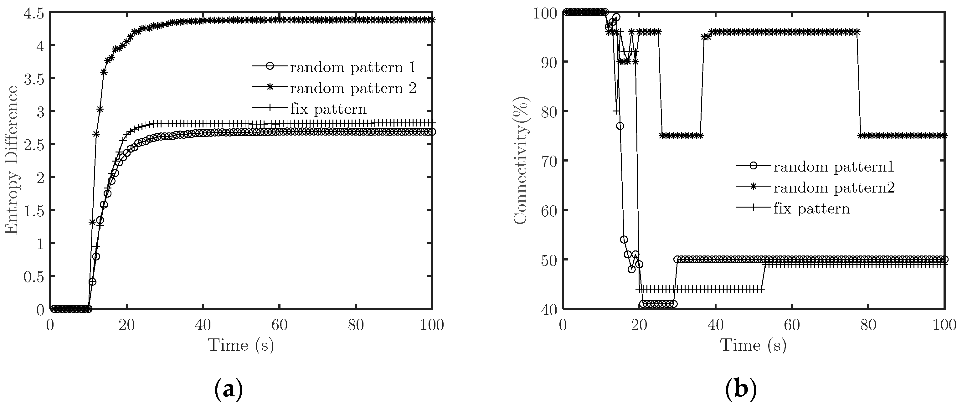
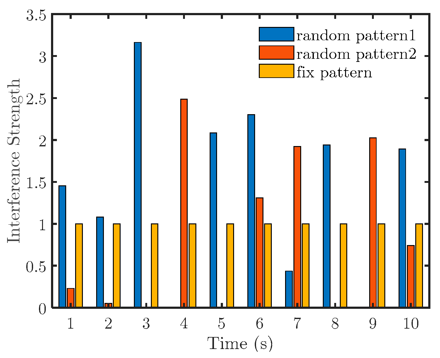
3.2.3. Effectiveness of Random and Regular Interference Patterns with Equal Average Intensity

Given the average interference signal strength, we conduct experiments with random and fixed interference patterns. For the random interference scenario, the intensity is set to be a random variable of a Gaussian distribution N( β , 1 ).
First, we set β = 1 to simulate medium-strength interference. Figure 7 depicts the simulation results of two random and one fixed pattern. The specific interference intensities are presented in Figure 8.
It is found that both suppressions are successful. From the viewpoint of the resulting topology of the target system, the splitting degree under the first random pattern is greater than the other two patterns. Furthermore, we consider the specific interference strength in Figure 8 for random pattern 1. The interference strength is high at the start of counteracting. This means that under the average power constraint, the high instantaneous interference strength should be arranged at the beginning of the counteraction.
Then, we set β = 0.25 to simulate the case of low average interference strength. Figure 9 illustrates some representative experimental results. After reducing the average intensity, the suppression behavior is successful when the interference pattern is fixed, which is uncertain when the interference pattern is random.
By further comparing the interference intensity (Figure 10), it is found that in case the interference fails, the signal strength is very low in the first few moments. Hence, to destroy the cooperative fly of the target system, a higher interference strength should be used at the beginning of the counteraction.

4. Anti-UAV Swarm through Suppression of Cooperative Fly

In terms of operation intent, the counteraction of UAV swarm cooperative fly can be divided into two types: destruction and delay. The former aims to destroy the target system and split it into several parts, and the latter is designed to extend the time for the target system to achieve cooperative flight. According to the experimental results in the previous section, the interference pattern with medium intensity and 100% duty cycle can be used to break cooperative flies. To delay cooperative flight, interference patterns with low intensity and 100% duty cycle can be used. What’s more, it is noted that the interference signal power should be increased to overcome the impact of path loss from the counterattack party to the target system. This paper proposes a unified suppression scheme that achieves different operational intent (delay or destroy) by setting different parameters.

4.1. Counteraction Algorithm for Cooperative Fly

The counterattack algorithm for cooperative fly is described in Algorithm 2.
Algorithm 2. Counterattack against Cooperative Fly
  ① Initialize connectivity threshold   δ c , and start monitoring. If the target system
is detected, go to step ②. Otherwise, go to step ①.
  ② Use Algorithm 1 to determine whether the target system starts the cooperative
fly. If it starts, go to step ③. Otherwise, go to step ②.
  ③ Measure the distance to the target cluster and calculate the path loss as [25]:
L o s s [ d B ] = 32.44 + 20 l o g d ( k m ) + 20 l g f ( M H z ) 20 l g A
where A is the path loss factor, usually set to 2 to 4, d is the distance to the UAV swarm,
and f is the operating frequency. The path loss is calculated as follows: l p a t h = 10 L o s s / 10 ;
  ④ Generate interference pattern I = [ I m , m = 1 , , M ] according to counter
intention and l p a t h and emit the interference signal. The interference pattern is as follows:
  4a. To delay cooperative fly, a low-intensity continuous jamming signal (i.e., duty
cycle 100%) is sent, and the equivalent noise figure is set to β = 0.25 , I m = β n 0 B l p a t h
  4b. To break the cooperative fly, the equivalent noise figure of medium intensity
continuous jamming signal (i.e., 100% duty cycle) is sent, and the equivalent noise figure
is set to β = 1   I m = k β 0 n 0 B l p a t h
  ⑤ Measure C ( t ) .
  If C ( t ) < δ c , or C ( t ) > δ c and the target system achieves cooperative fly, immediately
terminating the interference.
The flow chart is shown in Figure 11.

4.2. Simulations and Discussions

4.2.1. Countermeasures to Destroy Cooperative Fly

To destroy the cooperative fly, we set the algorithm’s parameters as follows: β = 1 , continuous interference with 100% duty cycle. The target UAV swarm comprises 100 individuals, and it starts the cooperative flight at 11th seconds and requires no less than 85% connectivity. Figure 12 and Figure 13 illustrate the simulation results.
In the experiment, the flight emergence is identified at the end of the 11th second, and the counterpart starts the interference immediately. At 19th seconds, the target system splits into 3 sub-clusters (Figure 13a). Since the connectivity is lower than the predefined threshold, it is determined that the counteraction is successful, and the interference signals immediately stop. After that, the target system splits more seriously. Figure 13b depicts the network’s topology at 10th seconds after stopping the interference. It is found that the system splits into five sub-clusters in this experiment.

4.2.2. Countermeasures to Delay Cooperative Fly

We set the algorithm’s parameters as follows to delay the target UAV swarm’s cooperative fly: β is 0.25, continuous interference with 100% duty cycle, and the intensity is equal. The simulation results are presented in Figure 14.
Figure 14 reveals that the target system achieves cooperative fly at 20th seconds, and the counterattack does not destroy the cooperative fly. The duration is T s u c = 9 s. Compared with the case without counterattack (which is also presented in Figure 14), the target system achieves cooperative fly at 17th seconds, and the duration is T s u c = 6 s. By emitting low-intensity interference, the counterattack prolonged the duration by 50%. It is to say the countermeasures achieved the desired effect. Further comparison of the system topology is illustrated in Figure 15.
The resulting system topology is quite different. With counterattack (Figure 15a), although the system is still connected, the node distribution is more dispersed, and thus the topology is more fragile. In comparison, when there is no counterattack mechanism (Figure 15b), the system after the cooperative fly is more robust. The counterattack with the continuous low-intensity in-band interference signal substantially damages the network’s stability, although the system is still connected. Moreover, due to the low average signal strength, it is difficult for the target system to differentiate this kind of interference from legitimate transmission scenarios.

5. Conclusions

This paper studies the countermeasures against UAV swarms from the perspective of suppressing cooperative flight. Specifically, we propose a dual threshold detection algorithm for cooperative flight. By monitoring the cooperative fly and network connectivity, the proposed algorithm can accurately identify the beginning, achievement, and failure of emergence, which provides a premise for the suppression algorithm. Moreover, we establish an in-band interference behavior model from the perspective of reducing channel capacity. Extensive experiments have been conducted to analyze the influence of different interference patterns. The results demonstrate that continuous low-intensity interference can effectively delay the process, which is not easy to be found by the target system, while moderate interference can destroy the cooperative fly. According to the two different operational intentions of delay and destruction, the UAV swarm’s suppression scheme is designed, and the effectiveness is verified by simulation.
In this paper, the UAV is assumed to be a particle. So, the constraint of UAV’s dynamic characteristics on its motion parameters, such as velocity and acceleration, are ignored, which limits the applicability of the research conclusions. To accurately model the motion of a target UAV is very difficult because the UAV suffers a lot of nonlinearities, couplings, under actuation, and disturbances. Fruitful work has been carried out [26,27] in the literature. In the future, the dynamic characteristics of typical UAVs will be considered to further improve the research in this paper.

Author Contributions

Conceptualization, X.Z.; methodology, X.Z.; software, X.Z.; validation, X.Z.; writing—original draft preparation, X.Z. and K.H.; writing—review and editing, X.Z. and Y.B.; visualization, X.Z.; project administration, X.Z.; funding acquisition, X.Z. All authors have read and agreed to the published version of the manuscript.

Funding

This research received was funded by Equipment Comprehensive Research, grant number 2021-42.

Data Availability Statement

Not applicable.

Acknowledgments

I sincerely thank all the reviewers for their valuable comments.

Conflicts of Interest

The authors declare no conflict of interest.

References

  1. Wu, T.; Feng, W.; Zhang, H. Research on the conceptual model of uav hive to sea combat. Command. Control. Simul. 2022, 44, 7–11. [Google Scholar]
  2. Niu, W.; Huang, J.; Miu, L. Research on the Concept and Key Technology of UAV Swarm to Sea Warfare. Command. Control. Simul. 2018, 40, 8–14. [Google Scholar]
  3. Walter, B.; Sammier, A.; Reiners, D.; Oliver, J. UAV Swarm Control: Calculating Digital Pheromone Fields with the GPU. J. Def. Model. Simul. 2006, 3, 167–176. [Google Scholar] [CrossRef]
  4. Ben, C. Gremlin Drone Recovered in Mid-Air for the First Time [OL]. Available online: https://newatlas.com/drones/gremlin-drone-recovery-mid-air/.2021.11 (accessed on 1 November 2021).
  5. Reilly, B. Gremlins program successfully retrieves drone in mid-flight. Inside Air Force 2021, 45, 1–32. [Google Scholar]
  6. Zhang, J.; He, Y.; Pan, X.; Qiao, Z.; Chen, H.; Shen, J.; Yang, Z. Vulnerability Analysis of UAV against Mesoband Electromagnetic Pulse. J. Proj. Rocket. Missiles Guid. 2020, 40, 110–115. [Google Scholar]
  7. Zhao, T.; Yu, D.; Zhou, D.; Chai, M.; He, K.; Zhou, C.; Wei, J. Ultra-wide spenctrum electromagnetic pulse effect and experimental analysis of UAV GPS Receiver. High Power Laser Part. Beams 2019, 31, 023001. [Google Scholar]
  8. Wang, T.; Peng, S.; Wang, G. Analysis of the Interference Mechanism of High PRF Pulse Jamming to the Front End of GPS Receiver. J. Air Force Early Warn. Acad. 2021, 35, 248–253. [Google Scholar]
  9. Fu, X.; Zhao, R.; Liang, Y.; Yan, Y. Review on the Development of Anti UAV Bee Colony Technology. J. CAEIT 2022, 17, 421–428. [Google Scholar]
  10. Hwang, S.P.; Kim, D.H. A Study on the Establishment of Anti-Drone system for the Protection of National Important Facilities. Soc. Digit. Policy Manag. 2020, 18, 247–257. [Google Scholar]
  11. Jie, C.; Miao, Z.; Ye, T. Research on the Development of Active Anti UAV System of US Army. Aerodyn. Missile J. 2020, 12, 36–42. [Google Scholar]
  12. Qiu, H.; Duan, H. From collective flight in bird flocks to unmanned aerial vehicle autonomous swarm formation. J. Eng. Sci. 2017, 39, 317–322. [Google Scholar]
  13. Zhao, H.; Gao, S.; Wang, H.; Yong, T.; Wei, J. Evaluation method for autonomous communication and networking capability of UAV. J. Commun. 2020, 41, 87–98. [Google Scholar]
  14. Qiu, H.; Duan, H.; Fan, Y.M. Unmanned aerial vehicle close formation cooperative control based on predatory escaping pigeon-inspired optimization. Sci. Sin. Technol. 2015, 41, 559–572. [Google Scholar]
  15. Liu, Q.; He, M.; Liu, J.; Xu, D.; Ding, N.; Wang, Y. A Mechanism for Identifying and Suppressing the Emergent Flocking Behaviors of UAV Swarms. Acta Electron. Sin. 2019, 047, 374–381. [Google Scholar]
  16. Liu, Q.; He, M.; Xu, D.; Ding, N.; Wang, Y. A Mechanism for Recognizing and Suppressing the Emergent Behavior of UAV Swarm. Math. Probl. Eng. 2018, 2018, 6734923. [Google Scholar] [CrossRef]
  17. Namuduri, K.; Wan, Y.; Gomathisankaran, M. Mobile Ad Hoc Networks in the Sky: State of the Art, Opportunities, and Challenges; Acm Mobihoc Workshop on Airborne Networks & Communications; ACM: New York, NY, USA, 2013. [Google Scholar]
  18. Tamas, V.; Andras, C.; Eshel, B.-J.; Cohen, I.; Shochet, O. Novel Type of Phase Transition in a System of Self-Driven Particles. Phys. Rev. Lett. 1995, 75, 1226–1229. [Google Scholar]
  19. Cheng, J.; Zhang, M.; Tang, J.; Kong, H. Emergence Quantitative Analysis of Complex Adaptive Systems Based on Shannon’s Information Entropy. J. Inf. Eng. Univ. 2014, 15, 270–274. [Google Scholar]
  20. Qu, Q.; He, X.; Lu, W. Emergence measurement of complex systems based on f-divergence. J. Acad. Armored Force Eng. 2017, 31, 106–110. [Google Scholar]
  21. Sheng, Z. Probability and Statistics, 3rd ed.; Higher Education Press: Beijing, China, 2001; Chapter 5. [Google Scholar]
  22. Hopcroftj, E.; Tarjan, R.E. Dividing a Graph into Triconnected Components. SIAM J. Comput. 1973, 2, 135–158. [Google Scholar] [CrossRef]
  23. Zhu, G.; Wei, G.; Pan, X.; Deng, X. Effects Research of Typical Communication Radio Radiated by Intraband Interference. J. Microw. 2011, 6, 93–96. [Google Scholar]
  24. Li, X.; Hao, X.; Han, H.; Zeng, Y.; Wang, L. Electromagnetic Interference Effect Research of Communication System Based on SER. J. Microw. 2017, 33, 71–76. [Google Scholar]
  25. Goldsmith, A. Wireless Communication; Posts Telecom Press: Beijing, China, 2007; pp. 35–36. [Google Scholar]
  26. Weng, Y.; Nan, D.; Wang, N.; Liu, Z.; Guan, Z. Compound robust tracking control of disturbed quadrotor unmanned aerial vehicles: A data-driven cascade control approach. Trans. Inst. Meas. Control. 2022, 44, 941–951. [Google Scholar] [CrossRef]
  27. Nan, D.; Weng, Y.; Wang, N. Data-driven robust PID control of unknown USVs. In Proceedings of the 2020 International Conference on System Science and Engineering (ICSSE), Kagawa, Japan, 31 August–3 September 2020. [Google Scholar]
Figure 1. The emergence intensity is measured by two existing methods. (a) Entropy difference of velocity angle; (b) Hel diversity of velocity angle.
Drones 07 00172 g001
Figure 2. The nodes’ position distribution at the beginning and the end of the experiments with different R. (a) Begin of simulation; (b) End of simulation (R = 50); (c) End of simulation (R = 25).
Drones 07 00172 g002
Figure 3. An interference pattern example.
Drones 07 00172 g003
Figure 4. Effectiveness comparisons of interference patterns with fixed signal strength and different duty cycles. (a) Emergence strength; (b) Connectivity.
Drones 07 00172 g004
Figure 5. Interference with a small duty cycle prolongs the synchronization duration. (a) Emergence strength; (b) Connectivity.
Drones 07 00172 g005
Figure 6. Effectiveness comparisons between the interference patterns with fixed average interference intensity and different interference. (a) Emergence strength; (b) Connectivity; (c) Nodes’ position distribution at the end of the simulation.
Drones 07 00172 g006
Figure 7. Effectiveness comparisons between random and regular patterns at medium strength ( β = 1 ) . (a) Emergence strength; (b) Connectivity.
Drones 07 00172 g007
Figure 8. Specification of the interference strength ( β = 1 ) .
Drones 07 00172 g008
Figure 9. Effectiveness comparisons between random and regular patterns at medium strength ( β = 0.25 ) . (a) Emergence strength; (b) Connectivity.
Drones 07 00172 g009
Figure 10. Specification of interference intensity ( β = 0.25 ) .
Drones 07 00172 g010
Figure 11. Flow chart of countermeasures against the cooperative fly of UAV swarm.
Drones 07 00172 g011
Figure 12. Effectiveness of the countermeasures to destroy cooperative fly. (a) Emergence strength (b) Connectivity.
Drones 07 00172 g012
Figure 13. Target system topology at different times. (a) the time when the counterattack mechanisms stop; (b) 10 s after the counterattack mechanisms stop.
Drones 07 00172 g013
Figure 14. Entropy difference of the target system with and without counterattack mechanisms.
Drones 07 00172 g014
Figure 15. Network topology after a cooperative flight with and without counterattack. (a) with countermeasures ( β is 0.25); (b) without countermeasures.
Drones 07 00172 g015
Disclaimer/Publisher’s Note: The statements, opinions and data contained in all publications are solely those of the individual author(s) and contributor(s) and not of MDPI and/or the editor(s). MDPI and/or the editor(s) disclaim responsibility for any injury to people or property resulting from any ideas, methods, instructions or products referred to in the content.

