Compressed Sensing-Based Genetic Markov Localization for Mobile Transmitters

Abstract

With the strengths of quickness, low cost, and adaptability, unmanned aerial vehicle (UAV) communication is widely utilized in the next-generation wireless network. However, some risks and hidden dangers such as UAV “black flight” disturbances, attacks, and spying incidents lead to the necessity of the real-time supervision of UAVs. A compressed sensing-based genetic Markov localization method is proposed in this paper for two-dimensional trajectory tracking of the mobile transmitter in a finite domain, which consists of three modules: the multi-station sampling module, the reconstruction module, and the localization module. In the multi-station sampling module, multiple stations are deployed to receive the signal transmitted by the UAV using compressed sensing, and the motion model of the mobile transmitter is the constant turn rate and acceleration (CTRA) model. In the reconstruction module, we propose a direct reconstruction method to extract the joint cross-spatial spectrum. In the genetic Markov localization module, we propose a two-step localization method to genetically correct the inaccurate points in the preliminary results and generate the tracking result. Extensive simulations are conducted to verify the effectiveness of the proposed method. The results show that the proposed method is superior to the particle filter method and the Markov Monte Carlo method at all sampling moments. Specifically, when SNR = 15dB, the root-mean-square error (RMSE) of the proposed method is $39\%$ and $60\%$ lower than that of the other two methods, respectively. Moreover, under the premise that the RMSE of the localization result is less than 30 m, the reconstruction module can reduce the running time of the proposed method by $33.3\%$.

1. Introduction

Unmanned aerial vehicles (UAVs) are known for their small size, easy operation, and flexibility. In recent years, UAV technology has continued to develop rapidly and has been utilized extensively in both military and civil fields [1,2]. The development of UAVs brings risks and hidden dangers at the same time. At present, nearly all of the leading countries in the world have had UAV “black flight” occurrence, which not only affects people’s lives and property safety, but also threatens the public safety and even air defense safety [3,4]. Owing to the risks of UAVs, it is now a primary priority for military and security organizations worldwide to efficiently and low-costly control unlawfully flying UAVs [5].

With the advancement of big data technology, collecting historical data of UAVs and then obtaining the behavior characteristics of UAVs has become a key exploration area. Therefore, this paper focuses on a UAV behavior prediction method to get real-time position data of UAVs. These data can help security agencies identify UAVs’ illegal behaviors and perform respective actions on time. Since there is no usable historical data for most of the trajectory prediction of illegal UAVs, this paper mainly discusses the passive localization method for mobile signals.

Passive localization is also called non-cooperative localization. The receiver in the localization system passively receives the target signal rather than actively radiating electromagnetic waves. After processing the received signal, the system gets the position estimation results to monitor, locate, and track target signals [6,7]. Compared with active localization, passive localization has superiority in concealment, battlefield viability, mobility, and cost. Passive localization can be divided into single-station localization and multi-station localization depending on the number of receivers in the system. The passive localization technology based on a single receiver requires repeated measurements to obtain sufficient parameter information, which makes it highly complex and unsuitable for variable UAV trajectory tracking. With information fusion further developed, multi-station passive localization has become a research hotspot with a wider detection range, higher system robustness, and superior performance [8]. The proposed method in this paper deploys multiple time-synchronized base stations to track the mobile signals and transmit the measurement results to a data center for information fusion via the network.

The common multi-station passive localization mechanisms include angle of arrival (AOA) [9,10], time of arrival (TOA) [8,11], time difference of arrival (TDOA) [12,13], frequency difference of arrival (FDOA) [14], and received signal strength (RSS) [15,16]. Various multi-station passive localization schemes using different mechanisms are given in [8,9,10,11,12,13,14,15,16]. The AOA-based scheme [9,10] collects the angle of arrival of the signal and does not require synchronization between base stations or data fusion. However, the receiver must have a directional antenna array, and it is unsuitable for accurate tracking of far-field transmitters such as UAVs. In the TOA-based localization scheme [8,11], the station measures the time of arrival of the signal. Although the TOA-based scheme is simple to operate and has good positioning accuracy, this scheme requires strict time synchronization of stations, which is challenging to meet in practice. In the TDOA-based localization scheme [12,13], the system detects the time difference of arrival of the signal, which only needs to keep the time synchronization between stations. The TDOA-based scheme has high localization accuracy, whereas the computational complexity is higher. The FDOA-based scheme [14] locates the target according to the Doppler frequency difference information generated by the mutual motion between the signal and the station. The RSS-based [15] scheme uses the correlation between signal propagation distance and energy loss. Based on the signal transmission model, it converts the received signal intensity into distance characteristics. Compared to other localization schemes, the RSS-based scheme has the lowest complexity and cost. Nevertheless, the localization accuracy may be undesirable owing to the shadow effect and long distance between the signal and the BSs [16].

The localization schemes mentioned above all estimate the parameters first, and then estimate the signal’s position depending on the results obtained, such as TDOA. However, the final estimation results are not assured to be optimal, particularly for the parameter estimation step. In [17], Xia et al. combined the particle filtering with the cyclic cross-spectrum for mobile co-channel signals to realize direct tracking. The experimental results show that the spectral function has a peak at the real signal position, demonstrating that the spatial spectrum is useful in signal localization. Considering the performance and computational complexity, we connect the localization method and the spatial spectrum to estimate the mobile signal’s position directly. The spatial spectrum and mobile signal position have a highly non-linear relationship in the Cartesian coordinates. Some improved Kalman filters are typically used to address the non-linear equations [18,19,20]. Extended Kalman filter (EKF) [18] is a recursive minimum mean square error estimation method. The method expands the nonlinear measurement equation with the Taylor formula to obtain the first-order linearization result. Therefore, the algorithm suffers from the error caused by linearization. The unscented Kalman filter (UKF) [19] utilizes the unscented transform algorithm, which can achieve higher accuracy, whereas the algorithm mode will be constrained by the Gaussian model. In [20], the centralized measurement fusion UKF (WMF-UKF) method is proposed, which is a universal weighted measurement fusion method. This method has a lower cost but also has linear error. Another popular estimation method for non-linear problems is the particle filter (PF) [21,22,23], which is based on a Bayesian framework. PF uses each particle and its corresponding weights to approximate the probability density function (PDF) of the target’s state at each moment and then updates the particle weights by the observed values to realize the tracking of the signal. Unfortunately, the introduction of resampling leads to the problem of particle degradation and particle scarcity. Liu in [24] proposed an adaptive Markov chain particle filtering algorithm, which discards the resampling and makes the particles converge faster, reduces the number of iterations, and obtains high accuracy in mobile source localization. Although the improved particle filter methods address the particle scarcity caused by resampling, they inevitably suffer from high computational complexity. Therefore, how to reduce the computational complexity of the algorithm while ensuring accurate mobile signal tracking is a topic worthy of study.

Compressed sensing is an effective technique to reduce running time and computational complexity [25,26]. In this paper, the compressed sensing uses random sampling to obtain discrete samples of the signal, discards the redundant information in the current signal sampling, and directly reconstructs the spatial spectrum function of the signal. It effectively reduces the redundancy of parameters, storage occupation, and computational complexity.

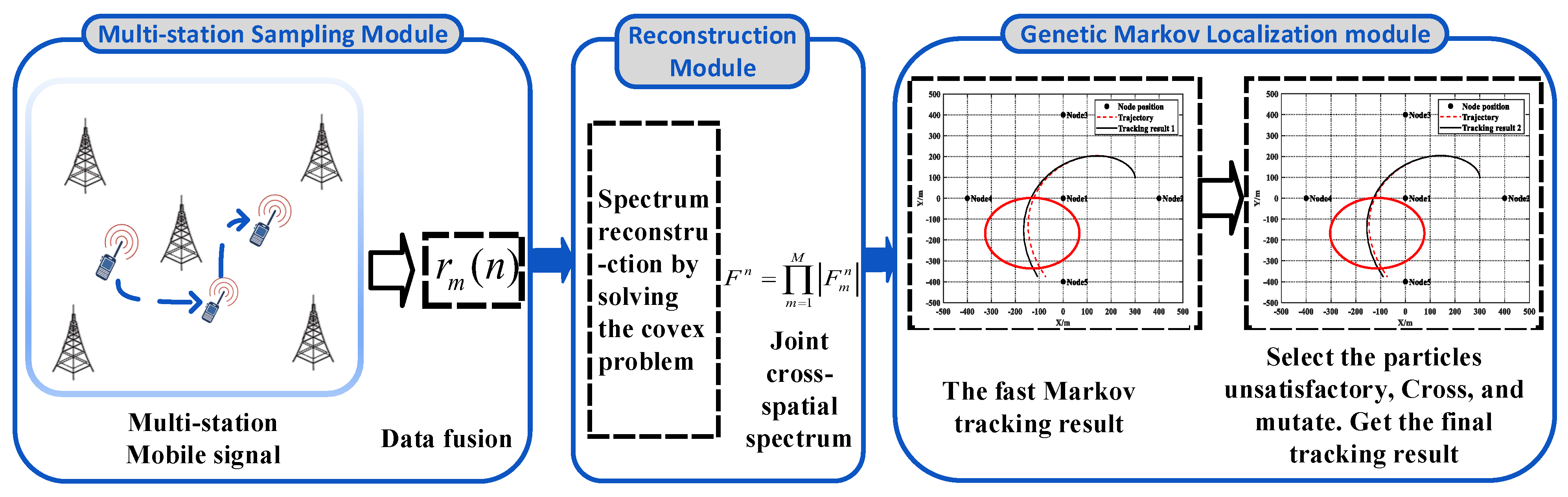
To summarize, a compressed sensing-based genetic Markov localization method is proposed for mobile transmitters in this paper. The re-sampling is not needed and therefore the particle degradation or depletion are nonexistent. Compared with other methods, the proposed method discards the redundant information and can achieve higher localization accuracy. The proposed method has three modules: the multi-station sampling module, the reconstruction module, and the genetic Markov localization module. The multi-station sampling module is designed to compressively sample the mobile signal and fuse the data from multiple stations. Furthermore, the reconstruction module links the multi-station sampling module and the genetic Markov localization module. The main contributions of this paper are as follows.

• We propose a compressed sensing-based localization method. After obtaining the signal data at a lower sampling rate, the cross joint spatial spectrum of the samples is recovered to directly estimate the position of the signal;
• Compared with the traditional particle filtering method, we proposed a genetic Markov method, which is a new two-step method. The inaccurate points in the preliminary results are genetically corrected and finally fused to generate the localization result;
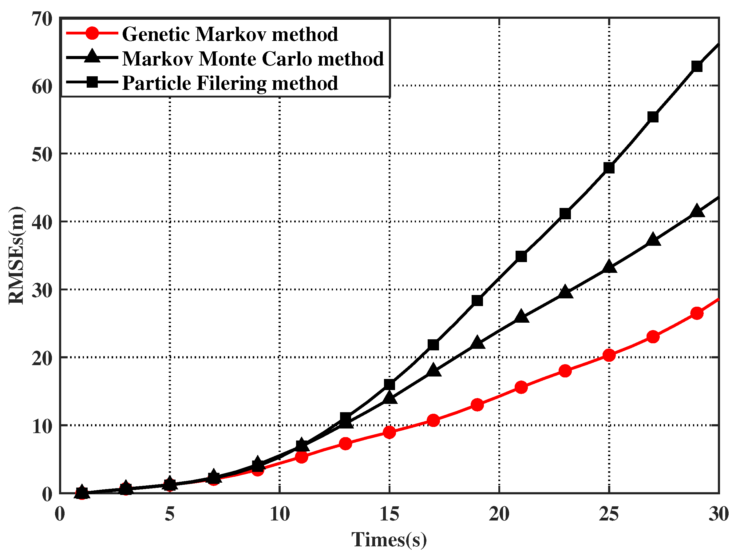
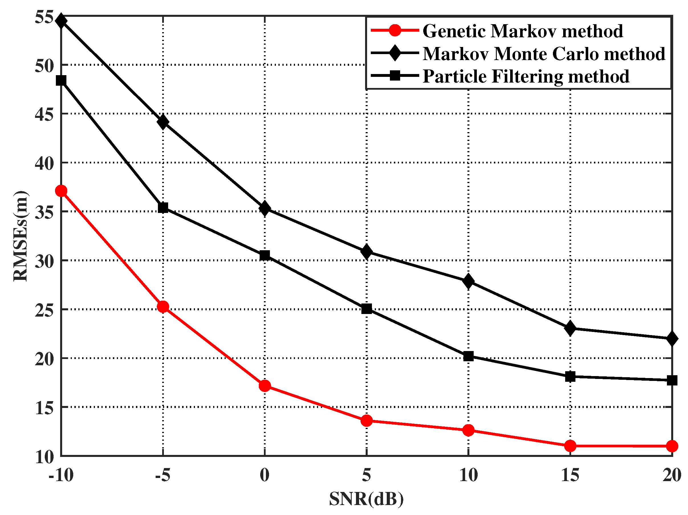
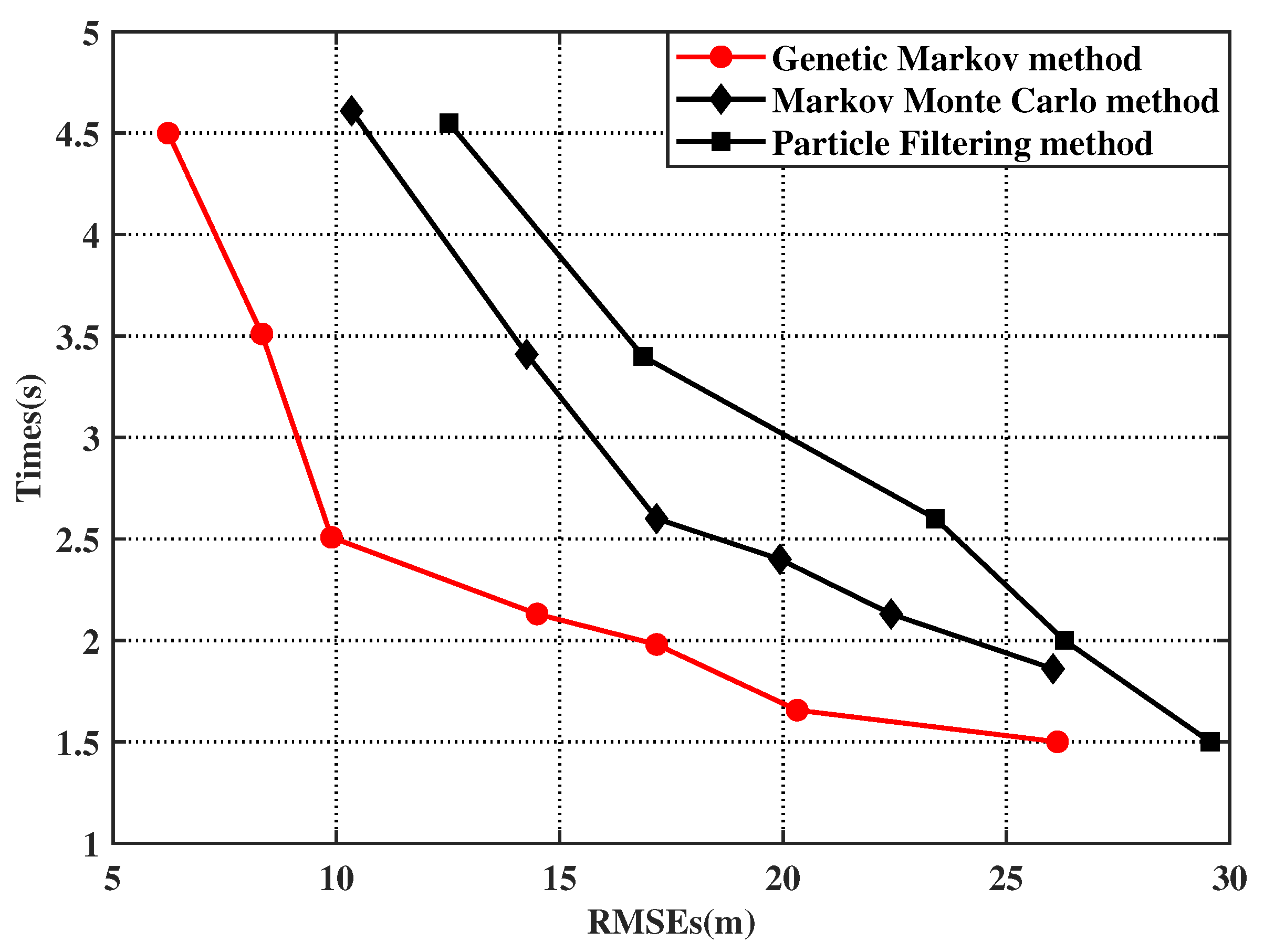
• Extensive simulations verify that the proposed method is superior to the particle filter method and the Markov Monte Carlo method. Under the same experimental environment, the proposed method can achieve higher accuracy in a shorter time.

The rest of the paper is organized as follows. Section 2 illustrates the system model and the proposed method framework. Section 3 introduces the proposed compressed sensing-based genetic Markov method. Simulations are conducted in Section 4. Section 5 concludes the paper, discusses the limitations of the method, and gives the future research direction.

2. System Model

Figure 1 presents the proposed method framework in this paper, which can coarsely be divided into three parts: multi-station sampling module, reconstruction module, and genetic Markov localization module.

In the multi-station sampling module, the signal is gathered by M$(M⩾3)$ scattered base stations (BSs) that are time-synchronized. The positions of BSs are fixed and described as $q_m={[x_m,y_m]}^T$, where $m=1,2,...,M$. The symbol $q_1$ represents the location of the reference BS. Make an assumption that each BS’s observations are independent of those of other BSs. After data fusion, the time-discrete signal at m-th BS and t-th snapshot can be modeled as:

$$r_{m,t}\left(n\right)={\alpha }_{m,t}{s}_t(n-D_{m,t})+v_{m,t}\left(n\right),n=1,2,\cdots ,N$$

(1)

$N=\lfloor f_s{T}_L\rfloor$ denotes the total number of the signal symbols in a snapshot, where $f_s$ is the sampling frequency, $T_L$ represents the sampling sustained time and $\lfloor ·\rfloor$ denotes the rounding down operator. The symbol ${\alpha }_{m,t}$ represents the amplitude attenuation changed with snapshot t. We assume that $v_{m,t}$ is the measurement noise, which is modeled by additive white Gaussian noise (AWGN) with zero mean and variance ${\sigma }^2$. Let $r_1$ be the reference signal, and the sample delay between the m-th BS and the reference is denoted by $D_{m,t}$. It can be expressed as

$$D_{m,t}=\frac{f_s}{c}(\parallel p_t-q_m\parallel -\parallel p_t-q_1\parallel )$$

(2)

where $p_t={[x_t,y_t]}^T$ is the position vector of the moving transmitter and c is the speed of the light. $\parallel ·\parallel$ denotes the Euclidean norm. The reference signal does not have a time delay. Namely, $D_{1,t}=0$.

Assume that the motion state of the mobile signal is modeled by CTRA model [27]. The vector $x\left(t\right)$ represents the motion state of the mobile signal, which can be described as follows in two-dimensional Cartesian coordinate.

$${\mathbf{x}}_t={[x_t,y_t,{\theta }_t,v_t,a_t,w_t]}^T,t=1,2,\cdots ,T$$

(3)

where $T_n$ denotes the total number of snapshots, the symbols a and w represent constant acceleration and turn rate, respectively. The position elements $x_t$ and $y_t$, the signal’s heading angle $\theta$, and the velocity v can be obtained based on the following state transition of the CTRA model:

$${\mathbf{x}}_t={\mathbf{x}}_{t-1}+\Delta {\mathbf{x}}_t+{\mathbf{w}}_t$$

(4)

where

$$\Delta {\mathbf{x}}_t={[{\dot{x}}_t,{\dot{y}}_t,w{T}_0,g{T}_0,0,0]}^T,$$

(5)

in which $T_0$ denotes the sampling interval, ${\dot{x}}_t$ and ${\dot{y}}_t$ are velocity elements with the following expressions, respectively.

$$\begin{array}{cc}\hfill {\dot{x}}_t=& \frac{1}{w^2}[(v_{t}w+gw{T}_0)sin({\theta }_t+w{T}_0)\hfill \\ \hfill & +gcos({\theta }_t+w{T}_0)-v_{t}wsin{\theta }_t-gcos{\theta }_t],\hfill \end{array}$$

(6)

$$\begin{array}{cc}\hfill {\dot{y}}_t=& \frac{1}{w^2}[(v_{t}w-gw{T}_0)cos({\theta }_t+w{T}_0)\hfill \\ \hfill & +gsin({\theta }_t+w{T}_0)+v_{t}wcos{\theta }_t-gsin{\theta }_t].\hfill \end{array}$$

(7)

Assume that the vector ${\mathbf{w}}_t$ is the process noise modeled by AWGN with zero mean and variance ${\Phi }_t$.

In the reconstruction module, we firstly initialize a set of random state particles from a given prior uniform distribution

$$x_1^n={[x_1^n,y_1^n,{\theta }_1^n,v_1^n,a_1^n,w_1^n]}^T,n=1,2,\cdots ,N$$

(8)

where N denotes the total number of particles. The position particles are denoted by $p_1^n={[x_1^n,y_1^n]}^T$, the TDOA particles $D_{m,1}^n$ can be obtained via replacing $p_t$ with $p_1^n$ in Equation (2). Then, the cross-spatial spectrum between the signals received by the mth BSs $r_m\left(n\right)$ and the reference $r_1\left(n\right)$ can be expressed as

$$F_m^n=\frac{1}{K}\sum _{k=1}^K{R}_1\left(k\right)R_m^H\left(k\right)e^{-i2\pi \frac{k}{K}{D}_m^n}$$

(9)

where $R_m\left(k\right)$ is the fast Fourier transform (FFT) of $r_m\left(n\right)$. Based on the assumption that each BS’s observations are independent of those of other BSs, the joint cross-spatial spectrum of multiple BSs can be described as

$$F^n=\prod _{m=1}^M\left|F_m^n\right|$$

(10)

In this paper, the system compressively samples the mobile signal, and the mathematical representation can be described as:

$$y_t\left(m\right)=\Phi x_t\left(n\right)$$

(11)

where $x_t\left(n\right)$ is an $N\times 1$ vector, $y_t\left(m\right)$ is an $M\times 1$ compressed sampling measurement vector, and $\Phi$ is an $M\times N$ compressed sampling matrix. Defining the compression rate as $M/N$, and then the compression gain can be defined as:

$$G=1-\frac{M}{N}$$

(12)

Reconstructing signal $x_t\left(n\right)$ from $y_t\left(n\right)$ is generally an under-determined problem. The sparse solution can be obtained by solving $l_0-norm$ optimization problem

$${∥minx∥}_{1}s.t.\Phi x=y$$

(13)

Reconstructing the joint cross-spatial spectrum is usually divided into two steps, first reconstructing the signal x and then obtaining the spectral function according to Equation (10). To further reduce the computational complexity, we reconstruct the spectral function directly from the compressed sampling signal. The FFT of y can be expressed as

$$Y\left(k\right)=\sum _{m=0}^{M-1}\Phi x\left(n\right)W_M^{mk},k=0,1,2,...,M-1$$

(14)

where $W_M^{mk}$ is the rotation factor. Combining Equation (14) and Equation (9), we get the result in Equation (15), where $X_k$ is the FFT of x,

$$F_m^n=\frac{1}{K}\sum _{k=1}^K\Phi X_1\left(k\right){\Phi }^H{X}_m^H\left(k\right)e^{-i2\pi \frac{k}{K}{D}_m^n}$$

(15)

After the joint cross-spatial spectrum of the signal is reconstructed, the system puts it into the genetic Markov localization module.

3. Proposed Method

In this paper, we propose the genetic Markov method, which is a two-step localization scheme. The inaccurate points in the preliminary results are genetically corrected and finally fused to generate the localization result. The proposed method has superiority in localization performance and computational complexity. The scheme first performs a fast Markov Monte Carlo method, whose efficiency depends on the transfer kernel, namely, the proposed density function (PDF). An appropriate proposed density will cause the Markov chain to converge quickly independent of the initial state. In most cases, the proposed density is a combination of the prior distribution and the probability of the approximate posterior distribution at the previous moment. However, this approach may not approximate the true distribution well in practical situations. The fast Markov Monte Carlo method samples from a rather convolutional version of the propagated PDF, which is constructed using gaussian approximation, with the following main steps.

Picking the initial state particles of the signal ${\left\{x_{k-1|k-1}^{\left(i\right)}\right\}}_{i=1}^N$ from the uniform distribution. The particle state at the next time ${\mathrm{x}}_{k|k-1}^{\left(i\right)}$ is obtained through Equation (4).

$$x_{k|k-1}^{\left(i\right)}\sim p\left(x\right|x_{k-1|k-1}^{\left(i\right)})$$

(16)

Computing the sample statistics:

$${\widehat{x}}_{k|k-1}=\frac{1}{N}{\sum }_{i=1}^N{x}_{k|k-1}^{\left(i\right)},$$

(17)

$$P_{k|k-1}=\frac{1}{N}{\sum }_{i=1}^N{x}_{k|k-1}^{\left(i\right)}{(\mathrm{x}}_{k|k-1}^{\left(i\right)}{)}^T-{\widehat{x}}_{k|k-1}{\widehat{x}}_{k|k-1}^T$$

(18)

Updating the measurements. For $i=1,...,N+M$, picking a sample $x_{k|k-1}^{{}^{\prime }}$ uniformly at random from particle set ${\left\{x_{k|k-1}^{\left(i\right)}\right\}}_{j=1}^N$, select a factory randomly $\epsilon \sim U({\epsilon }_1,{\epsilon }_2)$, then get the updated value of the particle from the distribution $x_{k|k}^{{}^{\prime }}\sim N(·|x_{k|k-1}^{{}^{\prime }},\epsilon P_{k|k-1})$. Set $\beta =\epsilon /(1+\epsilon )$, computing the acceptance probability of the new candidate according to Equation (19)

$$\begin{array}{c}\alpha (x^{{}^{\prime }},x^{\left(i\right)})=min\left\{1,\frac{p\left(z_k\right|x^{{}^{\prime }})}{p\left(z_k\right|x^{\left(i\right)})}\times \right.\hfill \\ \left.\frac{exp(-1/2{(x^{{}^{\prime }}-{\widehat{x}}_{k|k-1})}^T{P}_{k|k-1}^{-1}{(x^{{}^{\prime }}-{\widehat{x}}_{k|k-1})}^{\beta })}{exp(-1/2{(x^{\left(i\right)}-{\widehat{x}}_{k|k-1})}^T{P}_{k|k-1}^{-1}{(x^{\left(i\right)}-{\widehat{x}}_{k|k-1})}^{\beta })}\right\}.\end{array}$$

(19)

Generate a random number $u\sim U[0,1]$. If the random number is less than the acceptance, the particle will be updated, namely

$$x_{k|k}^{(i+1)}=x_{k|k}^{{}^{\prime }}$$

(20)

Otherwise, the update will not be accepted.

$$x_{k|k}^{(i+1)}=x_{k|k}^{\left(i\right)}.$$

(21)

After the update process is completed, discard the first M samples of the chain and compute the updated state estimation result

$${\widehat{x}}_{k|k}=\frac{1}{N}\sum _{i=1}^N{x}_{k|k}^{\left(i\right)}.$$

(22)

Next, for some inaccurate estimation results, we use the genetic method to correct them. It is a combination of the genetic method and the particle filtering, which introduces the selection, crossover, and mutation operations of the genetic method into particle filtering, and the specific implementation steps are as follows:

Select and calculate the weight variance of the particle set ${\left\{x_k^{\left(i\right)}\right\}}_{i=1}^N$ at the moment k to decide whether to optimize the result of this moment. For the results that need to be optimized, we divide the particles into two groups according to their weights. The group with a larger weight is retained and the group with a smaller weight is going to be crossed and mutated as follows.

$$x_k^i=\left\{\begin{array}{c}{C}_L\\ C_H\end{array}\right.\begin{array}{c}{\tilde{w}}_k^i⩽W\\ {\tilde{w}}_k^i>W\end{array}$$

(23)

where the threshold $W_T$ is the particle weight corresponding to the effective particle number. Then cross all particles in the low-weight group.

$$x_{kS}^l=\alpha x_{kL}^l+(1-\alpha )x_{kH}^j,$$

(24)

where the symbol $\alpha$ is the cross coefficient, representing the amount of information transferred from the low-weight group to the crossed particles.

Mutate to obtain new particles, which can increase the particle diversity.

$$x_{km}^l=\left\{\begin{array}{c}2x_{kH}^j-x_{kS}^l\\ x_{kS}^l\end{array}\right.\begin{array}{c}{r}_l⩽p_M\\ r_l>p_M\end{array}$$

(25)

where $p_M$ is the probability of variation and $r_l$ is the randomly selected coefficient of variation. The results are finally fused to generate the optimized estimation results. The genetic method can effectively address the particle degradation problem in the particle filtering algorithm and correct the inaccurate estimation points in the preliminary results.

4. Results and Discussion

4.1. Parameters Setting

In this section, extensive simulations are carried out to assess the performance of the proposed method, which is evaluated according to the scenario shown in Figure 1. The parameters settings are shown in

Table 1. Simulation parameters settings.

Parameters	Values
Modulation Type	QPSK
Carrier Frequency	$f_c=1.2\mathrm{GHz}$
Number of Base Stations	M = 5
Number of Particles	N = 400
Sample Interval	$T_0=1\mathrm{s}$
Sample Duration	$T_L=2\mathrm{ms}$
Number of Sampling Snapshots	$T_n=30$
Transmit Power	$10\mathrm{W}$
Initial State	${[300\mathrm{m},100\mathrm{m},\frac{\pi }{2}\mathrm{rad},4\mathrm{m}/\mathrm{s},2\mathrm{m}/{\mathrm{s}}^2,\frac{\pi }{25}\mathrm{rad}/\mathrm{s}]}^T$
Process Noise Covariance Matrix	diag$(5\mathrm{m},5\mathrm{m},0.1\mathrm{rad},0.1\mathrm{m}/\mathrm{s},0.2\mathrm{m}/{\mathrm{s}}^2,0.5\mathrm{rad}/\mathrm{s})$

.

Assume that the BSs and the mobile transmitter are in a region of $1\times 1{\mathrm{km}}^2$. The reference BS with the coordinate (0,0) is located in the center of the region. In each independent simulation, the remaining $M-1$ BSs are distributed at random. Throughout the sampling period, all BSs are assumed to be active and can simultaneously collect data from the mobile signal. After sampling, all data are sent to a fusion center for calculating the spatial spectrum. We use the CTRA model to describe the motion model of the mobile signal. The mobile signal’s trajectory begins at point P with the initial state ${[300\mathrm{m},100\mathrm{m},\frac{\pi }{2}\mathrm{rad},4\mathrm{m}/\mathrm{s},2\mathrm{m}/{\mathrm{s}}^2,\frac{\pi }{25}\mathrm{rad}/\mathrm{s}]}^T$. Assume that $P_1=10\mathrm{W}$ denotes the signal’s transmit power. The initial particles with a total number of N are generated from the following uniform distribution:

$$\begin{array}{c}{x}_1^n,y_1^n\sim \mathcal{U}(-0.5\mathrm{km},0.5\mathrm{km}),\hfill \\ {\theta }_1^n\sim \mathcal{U}(-\pi \mathrm{rad},\pi \mathrm{rad}),\hfill \\ v_1^n\sim \mathcal{U}(-10\mathrm{m}/\mathrm{s},10\mathrm{m}/\mathrm{s}),\hfill \\ a_1^n\sim \mathcal{U}(-5\mathrm{m}/{\mathrm{s}}^2,5\mathrm{m}/{\mathrm{s}}^2),\hfill \\ w_1^n\sim \mathcal{U}(-\frac{\pi }{2}\mathrm{rad},\frac{\pi }{2}\mathrm{rad}).\hfill \end{array}$$

(26)

4.2. Simulation Results

The tracking results of the mobile signal with the proposed method are shown in Figure 2. The solid black line in Figure 2 represents the trajectory of the signal, and the red dashed lines represents the tracking results. This paper performs a two-step localization method, Figure 2a,b represent the tracking results of the two steps, respectively. It can be seen that the inaccurate points in the preliminary results were corrected. The results verified the effectiveness of the genetic Markov method, as well as the significance of the study in this paper.

To further assess the performance of the proposed localization method, the root-mean-square error (RMSE) with $L=1000$ Monte Carlo simulations are calculated, and the RMSE of the estimation is described as

$$RMSE\left(t\right)=\sqrt{\frac{1}{L}\sum _{l=1}^L{∥p_l\left(t\right)-{\widehat{p}}_l\left(t\right)∥}^2},$$

(27)

where $p_l\left(t\right)$ is the position estimation in the l-th trial at the t-th time sample, and the ${\widehat{p}}_l\left(t\right)$ is the actual position of the mobile signal.

The performance of the proposed method with the different compressed gain are shown in Figure 3. As the compression degree increases, the running time of the method decreases. Relatively, the RMSEs of the method are larger at the same sample point. When the compression gain G = 0.4, the proposed method can provide satisfactory results.

Figure 4 shows the performance of the proposed method with the different number of particles at all sampling moments. It is clear that the more significant number of particles can lead to a lower RMSE at the same moment, the calculation of the method is more complex. After the number of particles reaches a certain value, the improvement of the method performance is no longer obvious.

The performance comparison of the proposed methods, the Markov Monte Carlo method and the particle filtering (PF) method are shown in Figure 5 and Figure 6. The PF [23] method generates a set of particles based on the empirical conditional distribution of the state vector, constantly adjusts the weight and position of the particles through resampling, and eventually gets the tracking result. The Markov Monte Carlo method [28] generates particles from the Markov chain without resampling, and updates particles based on acceptance probability to make the Markov chain stable and get the tracking result.

It is not difficult to find in Figure 5 that compared with the particle filtering method and the Markov Monte Carlo method, the proposed method can efficiently locate signals at all sampling moments. It can be seen in Figure 6 that the higher the SNR is, the lower the RMSE is and the better performance can be achieved. However, after the SNR is higher than 15 dB, the RMSE curve of the proposed method tends to be smooth. The RMSE of the proposed method in this paper is lower than other localization methods at different SNRs. It maintains higher estimation accuracy even if the SNR is low and shows good robustness. The running time comparison of the localization methods is illustrated in Figure 7. It is observed that the proposed method requires less running time than other compared methods for the same localization accuracy, illustrating the low computational complexity of the proposed method.

According to the simulation results above, the proposed method can provide efficient results for the tracking of mobile transmitters in a limited area. This can be explained by two aspects. Firstly, the proposed method selects the joint cross-spatial spectrum of the signal as the observation, which performs an obvious peak at the real signal position, and its robustness to the noise. Secondly, a two-step localization scheme is proposed, where the inaccurate results from the preliminary results are genetically corrected and fused to generate the final result. To reduce the computational complexity, the proposed method uses compressed sampling and directly reconstructs the spectral function. Compressed sensing can guarantee the accuracy of the results while effectively reducing the running time. Compared with other algorithms, the proposed method is superior in localization accuracy and running time.

5. Conclusions and Future Work

5.1. Conclusions

In this paper, a compressed sensing-based genetic Markov method was proposed for the mobile transmitter. The multi-station sampling module, the reconstruction module, and the genetic Markov localization module constitute the proposed method. Specifically, the multi-station module is deployed to receive the signal transmitted by the UAV using the compressed sensing and fuse data from different stations, and then the reconstruction module obtains the spatial spectrum directly from the compressed sampling data. Moreover, the genetic Markov localization module realizes the high accuracy tracking of the mobile signal. Finally, extensive simulations verified the superiority of the proposed method.

5.2. Future Work

The simulation results in Section 4 show that the proposed method can achieve high-accuracy localization in a limited area, demonstrating the validity of our study. Based on the study of this paper, our further research can consider more complex application scenarios. For instance, when the signal is moving at high speed, the Doppler frequency bias should be considered [29], multi-path channels may exist as well in an actual scenario [30]. Furthermore, altitude can be considered for the three-dimensional tracking of UAVs [31]. Although the study of this paper is a significant step in our research for UAV tracking, there are works to be done in the future.

References

1. Jiang, X.; Sheng, M.; Zhao, N. Green UAV communications for 6G: A survey. Chin. J. Aeronaut. 2022, 35, 19–34. [Google Scholar] [CrossRef]
2. Gupta, L.; Jain, R.; Vaszkun, G. Survey of Important Issues in UAV Communication Networks. IEEE Commun. Surv. Tutorials 2016, 18, 1123–1152. [Google Scholar] [CrossRef] [Green Version]
3. Zhang, J.; Zhang, K.; Wang, J. Current Status and Development Trend of Low-altitude Anti-UAV Technology. Aeronaut. Eng. Prog. 2018, 9, 1–8. [Google Scholar]
4. Sun, C. Application of Unmanned Aerial Reconnaissance Force in Special Operations. J. Ordnance Equip. Eng. 2011, 32, 40–42. [Google Scholar]
5. Jiang, C.; Fang, Y.; Zhao, P. Intelligent UAV Identity Authentication and Safety Supervision Based on Behavior Modeling and Prediction. IEEE Trans. Ind. Informatics 2020, 16, 6652–6662. [Google Scholar] [CrossRef]
6. Wan, P.; Huang, G.; Wang, J. Passive Localization of Signal Source Based on UAVs in Complex Environment. China Commun. 2020, 17, 107–116. [Google Scholar] [CrossRef]
7. Chaudhari, S.; Cabric, D. Cyclic Weighted Centroid Algorithm for Transmitter Localization in the Presence of Interference. IEEE Trans. Cogn. Commun. Netw. 2016, 2, 162–177. [Google Scholar] [CrossRef]
8. Gustafsson, F.; Gunnarsson, F. Mobile Positioning Using Wireless Networks: Possibilities and Fundamental Limitations Based on Available Wireless Network Measurements. Signal Process. Mag. IEEE 2005, 22, 41–53. [Google Scholar] [CrossRef]
9. Wang, Y.; Ho, V. An Asymptotically Efficient Estimator in Closed-Form for 3-D AOA Localization Using a Sensor Network. IEEE Trans. Wirel. Commun. 2015, 14, 6524–6535. [Google Scholar] [CrossRef]
10. Alma’aitah, A.; Alsaify, B.; Bani-Hani, R. Three-Dimensional Empirical AoA Localization Technique for Indoor Applications. Sensors 2019, 19, 5544. [Google Scholar] [CrossRef] [Green Version]
11. Sun, Y.; Ho, K.C.; Yang, Y. Computationally Attractive and Statistically Efficient Estimator for Noise Resilient TOA Localization. Signal Process. 2022, 200, 108663. [Google Scholar] [CrossRef]
12. Zhao, K.; Zhao, T.; Zheng, Z. Optimization of Time Synchronization and Algorithms with TDOA Based Indoor Positioning Technique for Internet of Things. Sensors 2020, 20, 6513. [Google Scholar] [CrossRef]
13. Ma, B.; Tong, C.; Tian, M. A TDOA Localization Method for Complex Environment Localization. J. Phys. Conf. Ser. 2021, 2004, 012003. [Google Scholar] [CrossRef]
14. Chan, Y.T.; Towers, J.J. Sequential Localization of A Radiating Source by Doppler-shifted Frequency Measurements. IEEE Trans. Aerosp. Electron. Syst. 1992, 28, 1084–1090. [Google Scholar] [CrossRef]
15. Patwari, N.; Ash, J.N.; Kyperountas, S. Locating the Nodes: Cooperative Localization in Wireless Sensor Networks. IEEE Signal Process. Mag. 2005, 22, 54–69. [Google Scholar] [CrossRef]
16. Liu, C.; Fang, D.; Yang, Z. RSS Distribution-Based Passive Localization and Its Application in Sensor Networks. IEEE Trans. Wirel. Commun. 2016, 15, 2883–2895. [Google Scholar] [CrossRef]
17. Xia, N.; Li, B.; Wang, J. Direct Tracking of Co-Channel Moving Sources With Different Cyclic Frequencies. IEEE Commun. Lett. 2020, 24, 1715–1718. [Google Scholar] [CrossRef]
18. Lee, K.; Oh, J.; You, K. TDOA-/FDOA-Based Adaptive Active Target Localization Using Iterated Dual-EKF Algorithm. IEEE Commun. Lett. 2019, 23, 752–755. [Google Scholar] [CrossRef]
19. Zhao, M.; Zhang, T.; Wang, D. A high precision indoor positioning method based on UKF. J. Intell. Fuzzy Syst. 2022, 42, 3639–3652. [Google Scholar] [CrossRef]
20. Gao, H.; Sun, S.; Li, Y. Nonlinear Weighted Measurement Fusion Unscented Kalman Filter with Asymptotic Optimality. Inf. Sci 2015, 299, 85–98. [Google Scholar]
21. Ryota, Y.; Ichiro, M.; Kenji, F. Particle Filter Design Based on Reinforcement Learning and Its Application to Mobile Robot Localization. Ieice Trans. Inf. Syst. 2022, 105, 1010–1023. [Google Scholar]
22. Samuel, L.S.; Nelyadi, S.S.; Aidan, F.B. Particle Filter Approach to Utilization of Wireless Signal Strength for Mobile Robot Localization in Indoor Environments. Int. J. Wirel. Mob. Netw. 2018, 10, 21–38. [Google Scholar]
23. Gordon, N.J.; Salmond, D.J. Novel Approach to Nonlinear/Non–Gaussian Bayesian State Estimation. IEE Proceedings. Part F 1993, 140, 107–113. [Google Scholar] [CrossRef] [Green Version]
24. Liu, J.; Han, C.Z.; Hu, Y. Adaptive MCMC Particle Filter for Tracking Maneuvering Target. In Proceedings of the Chinese Control Conference, Yantai, Chain, 22–24 July 2011; pp. 3128–3133. [Google Scholar]
25. Yu, X.; Wang, H.; Wu, J. A method of fingerprint indoor localization based on received signal strength difference by using compressive sensing. EURASIP J. Wirel. Commun. Netw. 2020, 2020, 839–848. [Google Scholar] [CrossRef] [Green Version]
26. Wang, J.; Fang, X.; Chen, Z. LCS: Compressive Sensing Based Device-free Localization for Multiple Targets in Sensor Networks. In Proceedings of the Proceedings IEEE INFOCOM, Turin, Italy, 14–19 April 2013; pp. 145–149. [Google Scholar]
27. Eltrass, A.; Khalil, M. Automotive Radar System for Multiple-vehicle Detection and Tracking in Urban Environments. IET Intell. Transp. Syst. 2018, 12, 783–792. [Google Scholar] [CrossRef]
28. Aharon, O.; Tslil, O.; Carmi, A. A Fast MCMC Particle Filter. In Proceedings of the 2018 21st International Conference on Information Fusion (FUSION), Cambridge, UK, 10–13 July 2018; pp. 1874–1881. [Google Scholar]
29. Liu, N.; Wang, R.; Zhao, Y. Computationally Efficient TDOA and FDOA Estimation Algorithm in Passive Emitter Localisation. IET Radar Sonar Navig. 2019, 13, 1731–1740. [Google Scholar] [CrossRef]
30. Xia, N.; Li, B.; Wang, J. A Direct Localization Method in the Presence of Cochannel Interference and Multipath Fading. IEEE Syst. J. 2020, 15, 2855–2858. [Google Scholar] [CrossRef]
31. Xia, N.; Xing, B. A Direct Localization Method for HF Source Geolocation and Experimental Results. IEEE Antennas Wirel. Propag. Lett. 2021, 20, 728–732. [Google Scholar] [CrossRef]
Figure 1. The proposed method framework.
Drones 07 00056 g001
Figure 2. The trajectory tracking results of the mobile signal: (a) tracking results of the fast Markov method; (b) tracking results after genetic correction.
Drones 07 00056 g002
Figure 3. Performance comparison of the proposed method versus the compressed gain G. (a) RMSE of the method versus the compressed gain G; (b) running time of the method versus the compressed gain G.
Drones 07 00056 g003
Figure 4. Performance comparison of the proposed method versus the number of particles N. (a) RMSE of the method versus number of particles; (b) running time of the method versus the number of particles.
Drones 07 00056 g004
Figure 5. Performance comparison of different localization methods at different sampling moments, with SNR = 20 dB.
Drones 07 00056 g005
Figure 6. Performance comparison of different localization methods versus SNRs.
Drones 07 00056 g006
Figure 7. The estimation time of different localization methods versus RMSEs.
Drones 07 00056 g007