Research on Adaptive Prescribed Performance Control Method Based on Online Aerodynamics Identification

Abstract

Wide-speed-range vehicles are characterized by high flight altitude and high speed, with significant changes in the flight environment. Due to the strong uncertainty of its aerodynamic characteristics, higher requirements are imposed on attitude control. In this paper, an adaptive prescribed performance control method based on online aerodynamic identification is proposed, which consists of two parts: an online aerodynamic parameter identification method and an adaptive attitude control method based on the pre-defined parameters of the control system. The aerodynamic parameter identification is divided into offline design and online design. In the offline design, neural networks are used to fit nonlinear aerodynamic characteristics. In the online design, a nonlinear recursive identification method is used to correct the errors of the offline fitted model. The adaptive attitude control is based on the conventional control method and updates the control gain in real time according to the desired system parameters to enhance the robustness of the controller. Finally, the effectiveness of the offline neural network and online discrimination correction is verified by mathematical simulations, and the effectiveness and robustness of the adaptive control proposed in this paper are verified by comparative simulation.

1. Introduction

Wide-speed-range vehicles play an important role in human space exploration activities. The vehicle is developing towards a wider speed domain, wider airspace, and longer range. The wide-speed-range vehicle has the characteristics of fast reaction speed, good maneuverability, and strong penetration ability, which can effectively conduct long-distance reconnaissance and strike targets, and greatly improve the long-range combat capability [1,2,3]. In the civil field, as a reusable aircraft, it can realize rapid transportation. It is the main tool for the development and utilization of adjacent space and has high economic value. The study of trajectory and attitude control for the wide-speed-range vehicle is one of the hot topics in current research [4,5].

At present, many scholars have carried out relevant research on attitude control of wide-speed-range vehicles, and the adaptive control method is the subject of active research interest [6,7,8,9]. In adaptive research, for the control design of deterministic systems, root locus, frequency characteristic method, and state space method are often used to ensure the stability of the system. For uncertain systems, it is usually required that the control system has adaptive adjustment capability and dynamically adjusts parameters according to certain indicators [10]. In other words, for the adaptive control of uncertain systems, it is a control method with online identification of model parameters.

Adaptive control requires wide-speed-range vehicles to be able to identify current aerodynamic characteristics, which requires online identification of aerodynamic parameters. Aerodynamic model identification can be divided into two categories: offline parameter identification and online parameter identification. The offline method refers to the identification analysis of the system after the data are obtained. It mainly focuses on the accuracy of system fitting and the accuracy of parameters influencing the law, without considering the time requirements; there are many methods available. Based on the input and output information of the aircraft motion model, traditional analysis methods include least squares, Kalman filter, maximum likelihood estimation, and their improvements, including output error method and equation error method [11,12,13,14]. However, traditional identification methods rely on the accurate identification model and reasonable initial value; otherwise, it is easy to trap the algorithm into local minimum value, and the error of offline analysis is large. In recent years, the rapid development of artificial intelligence technology, especially the maturity of neural network technology, has provided a new method for aircraft aerodynamic identification [15,16]. Neural networks can approximate any function with arbitrary precision, so the aerodynamic modeling process is avoided. In the process of aerodynamic parameter identification, the identification initial value is not required. When verifying the aerodynamic parameter identification results, the flight path does not need to be reconstructed.

The main purpose of online identification is to use the recursive identification method to satisfy timeliness. The aerodynamic parameter values are calculated recursively in real time after each new flight datum is collected by the airborne sensor. One of the most important purposes of online identification is to describe the characteristics of the aircraft dynamics that change with real-time control instructions. To meet this requirement, changes in multiple factors need to be considered, including flight conditions, engine thrust characteristics, aircraft configuration changes, various faults or damages, and other factors that affect aerodynamic characteristics. Real-time identification can be used for many tasks such as adaptive control logic design, stability test, flight envelope expansion, or safety monitoring [17,18,19,20]. Time domain identification methods include least squares aerodynamic parameter identification, extended Kalman filter aerodynamic parameter identification, and so on. The least squares method has a unique advantage in computational efficiency and is currently the most widely used time domain aerodynamic parameter identification method. In recent identification studies, the application of online identification mainly considers the improvement of the least squares method. On the one hand, starting from the nonlinear problem of the aerodynamic model, the method of multivariate orthogonal function is adopted to screen and updates the aerodynamic model according to a certain period [21]. On the other hand, considering the piecewise linearity of the model, this method considers that under certain conditions, the aerodynamic model is nearly linear and can be calculated by the linear method. After obtaining the piecewise aerodynamic parameters, a weighted method is used to combine several linear models in a nonlinear way [22].

When designing a traditional aircraft control system, the disturbance linearization of some important flight state points is expanded, and the control parameters are designed by using the pole configuration or trial-and-error method. As the complexity of the flight control system and the requirement of aircraft performance increase continuously, traditional design methods cannot handle the multi-input and multi-output complex system well [23]. With the development of control theory for nonlinear systems, the current design of aircraft control laws is based on more accurate nonlinear models, which makes the validation and evaluation of control simulation closer to the actual situation. At present, there are several main nonlinear adaptive control methods:

(1)

Gain preset method

The gain preset method is an important method for the transition from the linear control system to the nonlinear control system. This method still designs the control parameters at the state points, and the designed flight state points are more refined. During the flight process, high-dimensional interpolation is used to solve the current control gain based on the current flight state, such as angle of attack, speed, altitude, and so on. Su-27, Su-30, and F-16 aircraft have been successfully used in flight control systems [24,25,26,27].

(2)

L1 attitude control method

L1 adaptive control method is a new adaptive control architecture proposed by scholars Cao Chengyu and Naira Hovakimyan at the Control Conference in Minnesota in 2006 [28,29]. After this method was proposed, the application of L1 adaptive control method in the X-48B hybrid wing aircraft model was studied in Ref. [30]. NASA Dryden Flight Research Center proposed a design of an L1 adaptive control enhancement system with significant cross-coupling effect for MIMO nonlinear systems with mismatched uncertainties. The piecewise continuous adaptive law is adopted and extended to MIMO systems to explicitly compensate for dynamic cross-coupling [31].

(3)

Nonlinear Dynamic Inverse Method

The nonlinear dynamic inversion method is a model-based control method. Its control quality depends not only on the set control gain but also on the accurate dynamic model. It is more susceptible to the influence of uncertainties [32,33]. At present, Refs. [34,35] have improved the nonlinear dynamic inversion. Relevant work has been done on the hysteresis and control error, and the accuracy of attitude control in the case of model uncertainty has been improved. In NASA Langley Center research [36,37], aerodynamic identification is introduced into the nonlinear dynamic inversion, and an error observer is added to compensate for the identification and control errors. At present, the development goal of this method is to solve the problem of poor robustness.

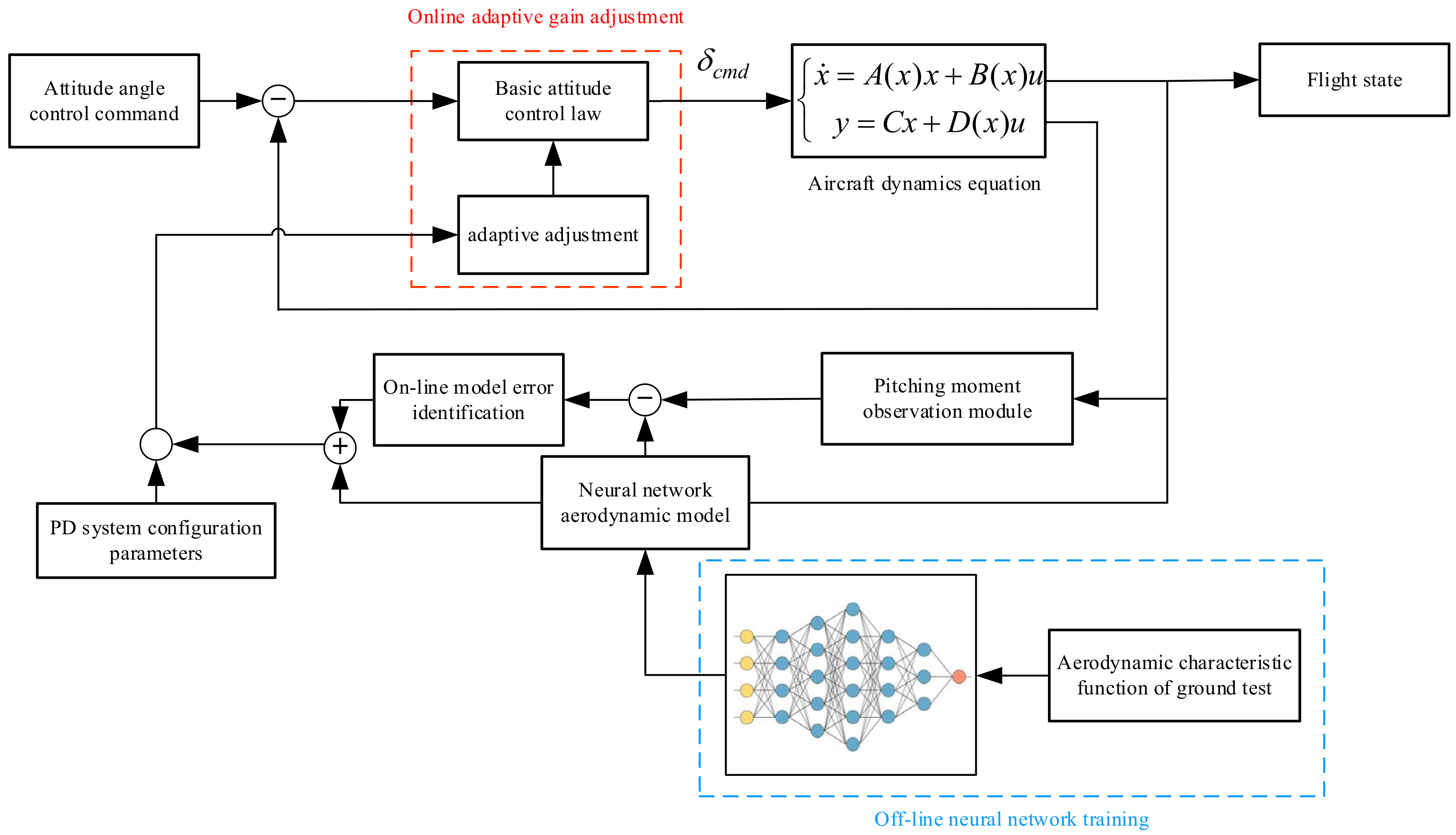
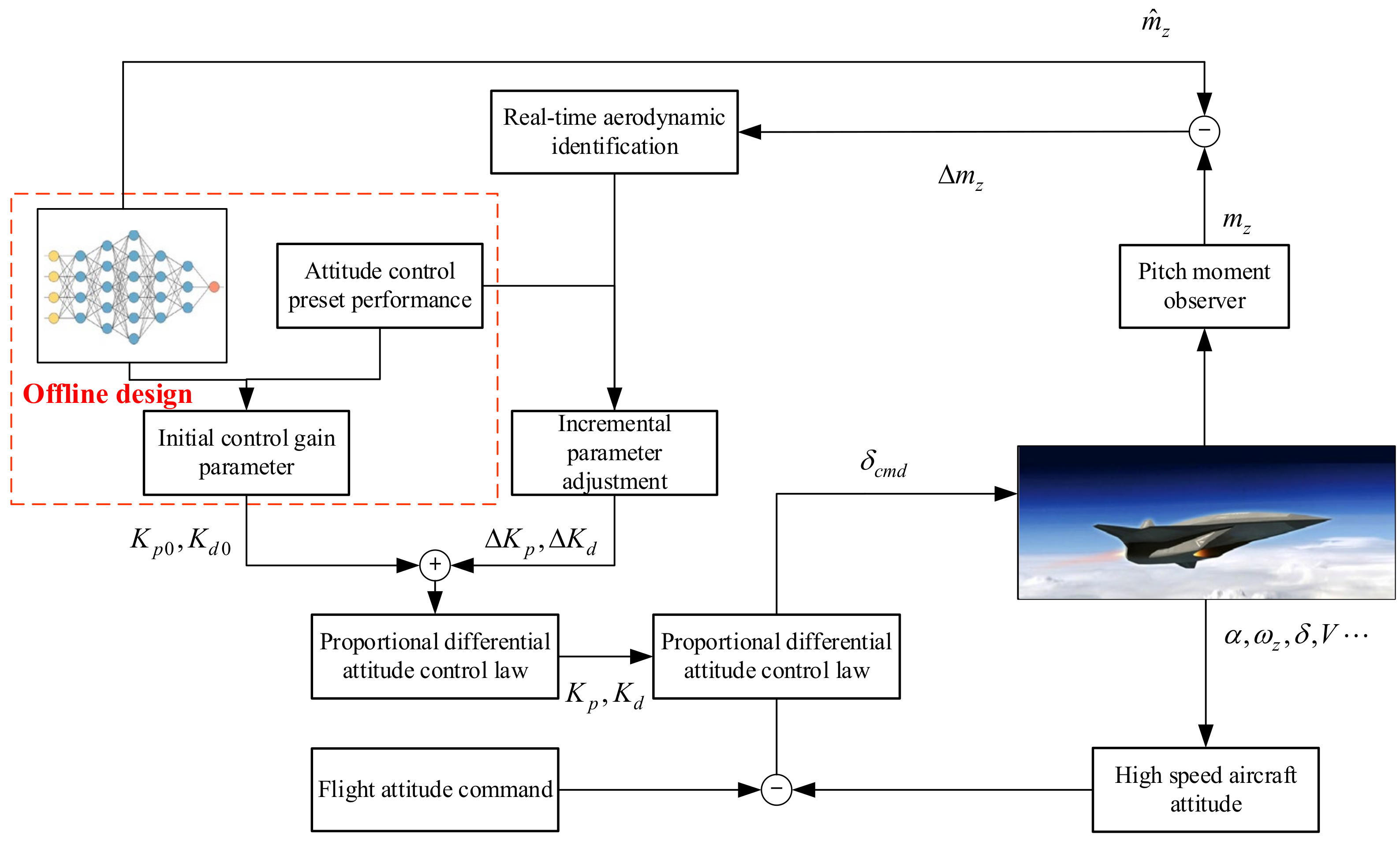
To summarize, online aerodynamic identification is mainly aimed at aerodynamic identification in a stable flight environment, and the method adopted is mainly based on multivariate orthogonal function and interval linearization. In the process of aerodynamic identification, the rudder surface excitation signal needs to be designed separately. In the study of adaptive control, the controller design relies on accurate aerodynamic and motion models. For nonlinear aerodynamic characteristics, the adaptive control can be corrected by designing state observers or correctors. For wide-speed-range vehicles, the excitation data of a stable environment cannot stimulate the aerodynamic characteristics of the entire process of the aircraft, and the design of the adaptive correction is relatively difficult due to the change in the flight environment. In this paper, offline intelligent learning and online error identification strategies are adopted to complete the acquisition of online aerodynamic parameters, and the traditional ground gain design method is applied to the online flight process. With the aerodynamic parameters and the expected parameters of the control system as the input, the control gain is updated in real time to improve the robustness of the system and simplify the complexity of the ground-segmented attitude control design.

The method presented in this paper has the following improvements over previous work: (1) In terms of aerodynamic parameter identification: the process of online stimulation required for the previous work is improved, and the method of combining incremental compensation based on the ground intelligent model reduces the amount of flight state data required for identification and accelerates the speed of parameter identification convergence. (2) In terms of adaptive control, the dependence of traditional adaptive methods on accurate models and the convergence requirements of adaptive laws are improved, and the adaptive parameter adjustment strategy is designed based on engineering control methods and combined with aerodynamic parameter identification results, so as to improve the robustness of the control system.

The rest of this paper is organized as follows: Section 2 explains the dynamic modeling and control method description of the wide-speed-range vehicle. Section 3 introduces the offline intelligent aerodynamic model learning method and online fitting error identification method. Section 4 describes the adaptive parameter adjustment method according to the preset performance. Section 5 provides the mathematical simulation comparison verification curve of the method. Section 6 presents the conclusion and future work directions.

2. Dynamic Modeling and Control Method Description of the Wide-Speed-Range Vehicle

2.1. Dynamic Modeling and Linearization

In the body axis system with the mass center of the wide-speed-range vehicle as the origin, the Newton Euler method is used to establish the linear motion equation under the combined external force and the angular motion equation under the combined external torque. In this paper, the longitudinal motion of the vehicle is mainly considered. According to the coordinate conversion relationship and force analysis, the motion equation of the longitudinal motion state is obtained, as shown in Equation (1):

$$\begin{array}{l}\left\{\begin{array}{c}m\frac{dV}{dt}=T\cos \alpha -D-mg\sin \theta \\ mV\frac{d\theta }{dt}=T\sin \alpha +L-mg\cos \theta \\ I_z\frac{d{\omega }_{}}{dt}=M_z\\ \frac{d\vartheta }{dt}=\omega \\ \frac{dH}{dt}=V\sin \theta \\ \alpha =\vartheta -\theta \end{array}\right.\\ M_z=qSc{m}_z,D=qS{c}_d,L=qS{c}_l\end{array}$$

(1)

where $V$ is the flight speed, $H$ is the flight altitude, m is the mass of the wide-speed-range vehicle, $T$ is the thrust, $D$ is the aerodynamic drag, $L$ is the aerodynamic lift, $g$ is the gravity, $\alpha$ is the angle of attack, $\theta$ is the trajectory inclination, $I_z$ is the rotational inertia, $M_z$ is the pitching moment, $\omega$ is the pitching angle rate, $\vartheta$ is the pitching angle, $q$ is the dynamic pressure, $S$ is the reference area, $c$ is the characteristic length, $m_z$ is the pitching moment coefficient, $c_d$ is the resistance coefficient, and $c_l$ is the lifting coefficient.

Pitching moment coefficient, lift coefficient, and drag coefficient are functions of flight state, which can be written as Equation (2), which will also be the main basis for the neural network fitting aerodynamic function, and the model basis for the online error recursive identification.

$$\left\{\begin{array}{c}{c}_d=f(V,H,\alpha ,\delta )\\ c_l=f(V,H,\alpha ,\delta )\\ m_z=f(V,H,\alpha ,\delta ,\omega ,\dot{\alpha })\end{array}\right.$$

(2)

The longitudinal motion of the wide-speed-range vehicle can be divided into two stages according to its disturbance response characteristics. The disturbance force on the centroid motion is relatively small compared with gravity, and the inertia is large. It is generally considered that the change of speed and height is a long-period motion; however, the disturbance torque of the wide-speed-range vehicle rotating around the center of mass is usually large, and the inertia is small. Therefore, it is considered that the angle and angular rate change rapidly, and that the movement of the wide-speed-range vehicle around the center of mass is a short period.

For attitude control, the law of angle change is usually studied. For the nonlinear differential equation model, it is usually converted into an ordinary differential equation for analysis according to the linearization expansion of the differential equation at a certain point; the assumption of small disturbance linearization is given below:

$$\begin{array}{l}\frac{d{x}_1}{dt}=f_1\left(x_1,x_2\cdots x_n\right)\\ \frac{d{x}_2}{dt}=f_2\left(x_1,x_2\cdots x_n\right)\\ \cdots \cdots \\ \frac{d{x}_n}{dt}=f_n\left(x_1,x_2\cdots x_n\right)\end{array}$$

(3)

The linearization assumption of small disturbances in a certain state $\left({\overline{x}}_1,{\overline{x}}_2\cdots {\overline{x}}_{\mathrm{n}}\right)$ is as follows:

$$\begin{array}{cc}\hfill & \frac{d\left(\Delta x_1\right)}{dt}=\frac{\partial }{\partial x_1}\left(f_1\left({\overline{x}}_1,{\overline{x}}_2\cdots {\overline{x}}_{\mathrm{n}}\right)\right)\Delta x_1+\cdots \frac{\partial }{\partial x_n}\left(f_1\left({\overline{x}}_1,{\overline{x}}_2\cdots {\overline{x}}_{\mathrm{n}}\right)\right)\Delta x_n\hfill \\ \hfill & \frac{d\left(\Delta x_2\right)}{dt}=\frac{\partial }{\partial x_1}\left(f_2\left({\overline{x}}_1,{\overline{x}}_2\cdots {\overline{x}}_{\mathrm{n}}\right)\right)\Delta x_1+\cdots \frac{\partial }{\partial x_n}\left(f_2\left({\overline{x}}_1,{\overline{x}}_2\cdots {\overline{x}}_{\mathrm{n}}\right)\right)\Delta x_n\hfill \\ \hfill & \cdots \cdots \hfill \\ \hfill & \frac{d\left(\Delta x_n\right)}{dt}=\frac{\partial }{\partial x_1}\left(f_n\left({\overline{x}}_1,{\overline{x}}_2\cdots {\overline{x}}_{\mathrm{n}}\right)\right)\Delta x_1+\cdots \frac{\partial }{\partial x_n}\left(f_n\left({\overline{x}}_1,{\overline{x}}_2\cdots {\overline{x}}_{\mathrm{n}}\right)\right)\Delta x_n\hfill \end{array}$$

(4)

Based on the establishment of the above dynamic model and the assumption of linearization of small disturbances, for the longitudinal channel, the linearized form of its short-period motion equation can be obtained as follows:

$$\left\{\begin{array}{c}\frac{d\Delta \alpha }{dt}=\Delta \omega +(-\frac{T+L_{\alpha }}{mV}+\frac{g\sin \theta }{V})\Delta \alpha -\frac{g\sin \theta }{V}\Delta \vartheta -\frac{L_{\delta }}{mV}\Delta \delta \\ \frac{d\Delta \omega }{dt}=\frac{M_{\alpha }}{I_{yy}}\Delta \alpha +\frac{M_{\omega }}{I_{yy}}\Delta \omega +\frac{M_{\delta }}{I_{yy}}\Delta {\delta }_e\\ \frac{d\Delta \vartheta }{dt}=\Delta \omega \end{array}\right.$$

(5)

2.2. Description of Attitude Control Method

As shown in Figure 1, the preset performance adaptive attitude controller based on online nonlinear error parameter identification is divided into two parts. In the ground design stage, aerodynamic characteristics are obtained according to the aircraft CFD or wind tunnel test, and the neural network method is used for fitting and training to establish the intelligent aerodynamic characteristics model. The other part is realized in the flight process. In the actual flight stage, the predicted value of the pitching moment is obtained according to the current flight state and the intelligent model. According to the flight state and body parameters, the real pitching moment value is obtained. The torque error is obtained by using the difference between the predicted value and the real value. According to the error and the flight state, the error is identified recursively in real time, and the error identification model is obtained. Finally, the control law parameters are adjusted by the compensated model and the controller preset performance.

3. Intelligent Aerodynamic Parameter Identification Method Based on Online Error Compensation

3.1. Aerodynamic Characteristics of Neural Network

The neural network is a mainstream method of current artificial intelligence technology, and its derivative technologies such as function fitting, differential equation solving, image recognition, time series prediction, etc., have been widely used in many engineering fields. In the research of this paper, the neural network is used to map and fit flight state and aerodynamic parameters to replace the aerodynamic function interpolation module obtained from ground test to solve aerodynamic parameters, which greatly improves the calculation efficiency while ensuring the original calculation accuracy, thus giving the original method stronger online calculation and adaptive ability.

3.1.1. Neuron, Activation Function, and Loss Function

The node in the neural network is the neuron, which is the basic unit of the neural network. The sum calculation, activation function, and offset value are defined on the neuron, and the weight is defined on the directed connection. When the data are input to the neuron through the connection, it is necessary to sum all inputs first, and then add the offset value on the neuron. The bias value is updated during the training of the neural network [38].

The activation function is a calculation function acting on the neuron. Its main function is to increase the nonlinearity of the neural network calculation. After the introduction of the activation function, the neural network has the fitting ability of any nonlinear function. The commonly used activation function for neural network training is sigmoid, which is also called the logistic function. It is a monotone-increasing function with a range of (0, 1). The definition is given by Formula (6)

$$S\left(x\right)=\frac{1}{1+e^{-x}}$$

(6)

The sigmoid function can be derived everywhere, and its derivative is:

$$S^{\prime }\left(x\right)=\frac{e^{-x}}{{\left(1+e^{-x}\right)}^2}=S\left(x\right)\left(1-S\left(x\right)\right)$$

(7)

In neural networks, the commonly used loss functions are mean square error (MSE), which are given by Formula (8).

$$L_{MSE}=\frac{1}{N}{\displaystyle \sum _{i=1}^N{\left[Y_i-f\left(X_i\right)\right]}^2}$$

(8)

In the formula, $N$ represents the number of samples, $X_i$ he represents the input sample, $Y_i$ represents $X_i$ corresponding label, and $f\left(X_i\right)$ represents the predicted output of the neural network when the input is $X_i$.

The deviation between the current network model and the expected network model is described by the loss function. The process of neural network training is to make the value of the loss function approach zero. The value of the loss function can also be used as the termination mark of the neural network training. When $L$ is less than the preset tolerance error, it is considered that the neural network model has enough precision to terminate the network training.

3.1.2. Input Layer, Output Layer, and Hidden Layer

The neurons in the neural network are arranged in layers as shown in Figure 2. According to the position of the neurons in the network, the first layer of neurons is called the input layer, the last layer of neurons is called the output layer, and several layers of neurons in the middle are called the hidden layer.

3.1.3. Training Set, Test Set, and Verification Set

To make the neural network work, enough sample data are needed. Data are usually divided into two parts: one part is used to train the neural network, which generally accounts for more than 90% of the total data. The other part is used for neural network performance testing, which generally accounts for less than 10% of the total data, and is also known as a verification set.

Before the implementation of neural network training, the data used for training will be further divided into two parts. One part is used for both forward propagation and backpropagation to update the network parameters. This part is called the training set. The other part only conducts forward propagation to verify whether the error of the neural network has converged to the preset tolerance. This part of the data is called the test set.

3.1.4. Forward Propagation and Backpropagation

Given the input signal, the process of obtaining the output signal through neural network calculation is called forward propagation. In the forward propagation process, the input signal first comes to the input layer and does not perform any operation. After that, it is transferred from the input layer to the first layer of the hidden layer, then the second layer of the hidden layer, until the output layer. In these processes, multiplication, summation, addition, and activation will be performed in each neuron transmitted by each layer.

Back propagation is the process of updating the network parameters during neural network training. To perform backpropagation, first perform forward propagation to obtain the error of the network prediction value described by the loss function and the database tag value, and then obtain the partial derivative of the error at each layer. Then, use the gradient descent method to update the parameters of the neural network, and finally achieve the training goal of making the loss function close to zero.

Suppose that the output of each network layer after activation is $f_i(x)$, where i is the layer i, and x represents the input of layer i; that is, the output of layer i − 1, and f is the activation function. Then, it can be concluded that:$f_{i+1}=f(w_{i+1}{f}_i+b_{i+1})$.Define the loss function as L; \the weight is updated based on error backpropagation as follows:

$$\begin{array}{l}\left\{\begin{array}{c}\frac{\partial L}{\partial w_i}=\frac{\partial L}{\partial f_i}\frac{\partial f_i}{\partial w_i}=\frac{\partial L}{\partial f_i}{f^{\prime }}_i{f}_{i-1}\\ \frac{\partial L}{\partial f_i}=\frac{\partial L}{\partial f_{i+1}}\frac{\partial f_{i+1}}{\partial f_i}\end{array}\right.,1\le i\le k-1\\ \Delta w_i=-\eta \frac{\partial L}{\partial w_i}\end{array}$$

(9)

In the above formula, the initial value of the loss function, that is, the error of the output layer feedback, is the error between the neural network output and the expected output.

3.2. Recursive Least Squares Online Error Identification

Due to the discrepancy between the aerodynamic model obtained from ground tests and the real aerodynamics during real flight. At the same time, considering that the range of input information required by the neural network model is extremely strict, if the state beyond the input range of ground training occurs during flight, the predicted aerodynamic coefficient error is large. Therefore, the aerodynamic model error is considered as the input information of the online identification algorithm, and the offline model is compensated by the real-time recursive identification algorithm.

To illustrate the recursive least square (RLS), the basic idea of the least square method is introduced. For the model parameter estimation problem, if the relationship between the output and the model parameters is given by the following equation, the model is called a linear parameter model.

$$\mathit{z}=\mathit{H}\mathit{a}+\mathit{V}$$

(10)

The optimal estimation of the parameter $\mathit{a}$ by using the least square method is:

$$\mathit{a}={({\mathit{H}}^{\mathit{T}}\mathit{H})}^{-1}{\mathit{H}}^{\mathit{T}}\mathit{z}$$

(11)

With the continuous increase in observation information, the accuracy of estimates will be higher and tends to be stable, which is also one of the means to test the accuracy of estimates. However, if the common least square (LS) method is used, the calculation workload will increase with the increase of observation information. It can also be seen from the following analysis that because every calculation requires all the information, the previous calculation process is repeated. To overcome this shortcoming, recursive least square (RLS) is introduced.

According to the basic form of the least square method, the discrete observation equation of the system at time $k$ is:

$$z(k)=\mathit{H}(k)\mathit{a}+v(k)$$

(12)

where $v(k)$ is the measurement noise

Including the time $k$ and the previous total observation equation, denoted as:

$${\mathit{z}}_k={\mathit{H}}_k\mathit{a}+{\mathit{V}}_k$$

(13)

When new observation data are added, the above equation is rewritten as:

$$\mathit{z}(k+1)=\mathit{H}(k+1)\mathit{a}+v(k+1)$$

(14)

So, the overall observation equation becomes the following form:

$${\mathit{z}}_{k+1}={\mathit{H}}_{k+1}\mathit{a}+{\mathit{V}}_{k+1}$$

(15)

If the traditional least squares method is continued, when $k+1$ times of observation data are involved in the calculation, the discrete observation data of the $n(n<k+1)$ times needs to be repeated for $k-n+2$ times. With the increase in the amount of observation data, the amount of repeated calculation will increase, making the calculation efficiency lower and lower.

To overcome this shortcoming, the recursive method is used to estimate parameter ${\widehat{a}}_{j+1}$ based on the parameter estimation ${\widehat{a}}_j$ and with the new information.

$$\begin{array}{c}{\mathit{H}}_{k+1}^T{\mathit{H}}_{k+1}={\left[\begin{array}{c}{\mathit{H}}_k\\ \mathit{H}(k+1)\end{array}\right]}^T\left[\begin{array}{c}{\mathit{H}}_k\\ \mathit{H}(k+1)\end{array}\right]\\ \hspace{1em}\hspace{1em}\hspace{1em}\hspace{1em}\hspace{1em}\hspace{1em}={\mathit{H}}_k^T{\mathit{H}}_k+{\mathit{H}}^T(k+1)\mathit{H}(k+1)\end{array}$$

(16)

Matrix inversion formula is introduced:

$${(\mathit{A}+\mathit{C}{\mathit{C}}^T)}^{-1}={\mathit{A}}^{-1}-{\mathit{A}}^{-1}\mathit{C}{(I+{\mathit{C}}^T{\mathit{A}}^{-1}\mathit{C})}^{-1}{\mathit{C}}^T{\mathit{A}}^{-1}$$

(17)

Definition $\mathit{P}={({\mathit{H}}^T\mathit{H})}^{-1}$, according to the matrix inversion formula

$$\begin{array}{c}\mathit{P}(k+1)=\mathit{P}(k)-\mathit{P}(k){\mathit{H}}^T(k+1)\cdot \\ \hspace{1em}\hspace{1em}\hspace{1em}\hspace{1em}\hspace{1em}\hspace{1em}\hspace{1em}\hspace{1em}\hspace{1em}\hspace{1em}\hspace{1em}\hspace{1em}{\left[I+\mathit{H}(k+1)\mathit{P}(k){\mathit{H}}^T(k+1)\right]}^{-1}\mathit{H}(k+1)\mathit{P}(k)\end{array}$$

(18)

Lead-in gain matrix $K$

$$\mathit{K}(k+1)=\mathit{P}(k){\mathit{H}}^T(k+1){\left[\mathit{I}+\mathit{H}(k+1)\mathit{P}(k){\mathit{H}}^T(k+1)\right]}^{-1}$$

(19)

By combining Equations (18) and (19), it can be obtained that

$$\mathit{P}(k+1)=\mathit{P}(k)-\mathit{K}(k+1)\mathit{H}(k+1)\mathit{P}(k)$$

(20)

By combining Equations (11), (15), (19) and (20), we can obtain

$$\mathit{a}(k+1)=\mathit{a}(k)+\mathit{K}(k+1)[\mathit{z}(k+1)-\mathit{H}(k+1)\mathit{a}(k)]$$

(21)

In summary, the recursive formula is (19)–(21).

According to the above-established aerodynamic characteristic error modeling function and the derived recursive least square formula, the aerodynamic coefficient estimation of the actual flight state can be obtained.

4. Adaptive Prescribed Performance Control Based on Aerodynamic Parameters

4.1. Adaptive Gain Adjustment Strategy Based on Aerodynamic Identification

The adaptive attitude control method adopted in this paper is based on aerodynamic parameters and the prescribed performance of the closed-loop system. The strategy of off-line training and online error compensation is used to identify aerodynamic parameters to obtain the aerodynamic model of real-time flight, which is introduced in Section 3. This section describes the adaptive control gain adjustment strategy. In traditional control methods, the proportional term acts on the error between the command value and the state value, which is closely related to the adjustment time of the system; the differential term acts on the error rate, which changes the damping characteristic of the system and determines the dynamic response of the system; and the integral term acts on the error accumulation, which is related to the steady-state characteristic of the system. For the aerodynamic characteristics of aircraft, the static stability coefficient, control coefficient, and damping coefficient correspond to the dynamic characteristics and response speed of the system, respectively. Therefore, the adaptive gain adjusts the proportional and differential terms in the traditional control. The adaptive control block diagram based on aerodynamic parameter identification is as Figure 3.

4.2. Design of Adaptive Gain Adjustment Control for Wide-Speed-Range Vehicle

In short-period motion, the quality of attitude control is significantly affected by uncertain disturbances. The method of combining preset performance control with real-time aerodynamic parameter identification is adapted to dynamically adjust the control gain to improve the robustness of the control system. First, according to Equation (5), the linearized ordinary differential equation can be rewritten into the state space expression to facilitate the writing of the closed-loop system equation and the solution of key parameters. The state space expression of the longitudinal motion of the wide-speed-range vehicle is:

$$\left[\begin{array}{c}\Delta \dot{\vartheta }\\ \Delta \dot{\omega }\\ \Delta \dot{\alpha }\end{array}\right]=\left[\begin{array}{ccc}0& 1& 0\\ 0& \frac{M_{\omega }}{I_z}& \frac{M_{\alpha }}{I_z}\\ -\frac{g\sin \theta }{V}& 1& (\frac{g\sin \theta }{V}-\frac{T+L_{\alpha }}{mV})\end{array}\right]\left[\begin{array}{c}\Delta \vartheta \\ \Delta \omega \\ \Delta \alpha \end{array}\right]+\left[\begin{array}{c}0\\ \frac{M_{\delta }}{I_z}\\ -\frac{L_{\delta }}{mV}\end{array}\right]\Delta \delta$$

(22)

To track the pitch angle command solved by the altitude control loop, the command tracking control is usually realized through the deflection of the control surface. According to the idea of PD control, the control equation is as follows (22):

$$\Delta \delta =K_p\Delta \vartheta +K_d\Delta \omega$$

(23)

To facilitate system analysis and parameter solution, simplify the state space model:

(1)

According to the small disturbance linearization method, the motion state in horizontal flight is expanded linearly, so the trajectory inclination is about 0.

(2)

Because the momentum of the wide-speed-range vehicle is very large during flight, it is considered that the change of attack angle is consistent with that of pitch angle in short-period motion.

$$\frac{L_{\delta }}{mV}\approx 0,\frac{g\sin \theta }{V}\approx 0,\frac{T+L_{\alpha }}{mV}\approx 0$$

(24)

Therefore, after adding PD control, the closed-loop characteristic equation of the system is as follows:

$$s[s^2-(\frac{M_{\omega }}{I_z}+\frac{M_{\delta }}{I_z}{K}_d)s-(\frac{M_{\delta }}{I_z}{K}_p+\frac{M_{\alpha }}{I_z})]=0$$

(25)

According to the characteristics of the second-order system, from the above system it can be known that regulating $K_P$ changes the natural frequency, which is related to the response rate of the system, and regulating $K_d$ changes the damping ratio of the system, which is related to the transition process of the system. Given the expected damping ratio and natural frequency of the system: ${\xi }^{\ast }$ and ${\omega }_n^{\ast }$, the characteristic equation of the second-order system can be known from the above as $s^2+2{\xi }^{\ast }{\omega }_n^{\ast }s+{\omega }_n^{\ast }{}^2=0$, and there is a $K_{p,t}$ and $K_{D,t}$ corresponding to any group of aerodynamic data $M_{\omega },M_{\alpha },M_{\delta }$:

$$\left\{\begin{array}{l}{K}_{P,t}=-\left({\omega }_n^{\ast }{}^2-\frac{M_{\alpha }}{I_z}\right)/\frac{M_{\delta }}{I_z}\hfill \\ K_{D,t}=-\left(2{\xi }^{\ast }{\omega }_n^{\ast }+\frac{M_{\omega }}{I_z}\right)/\frac{M_{\delta }}{I_z}\hfill \end{array}\right.$$

(26)

When the aerodynamic identification updates the corresponding aerodynamic derivative value, the expected proportional and differential gain can be approached step by step through iterative adjustment. The updated equation is as follows:

$$\left\{\begin{array}{l}{K}_P\left(i+1\right)=K_P\left(i\right)+\lambda \left(K_{P,t}-K_P\left(i\right)\right)\hfill \\ K_D\left(i+1\right)=K_D\left(i\right)+\lambda \left(K_{D,t}-K_D\left(i\right)\right)\hfill \end{array}\right.$$

(27)

Stability analysis:

It can be seen from the above that the closed-loop characteristic equation of the system can be written as $s[s^2-(\frac{M_{\omega }}{I_z}+\frac{M_{\delta }}{I_z}{K}_d)s-(\frac{M_{\delta }}{I_z}{K}_p+\frac{M_{\alpha }}{I_z})]=0$. According to the characteristics of the second-order system, when its coefficients are greater than zero, the system will remain stable for this system.

According to the above algorithm, there is a corresponding $M_{\omega },M_{\delta },M_{\alpha }$ for a given group of aerodynamic data. At this time, the characteristic equation can also be written as $s^2+2\xi {\omega }_{n}s+{\omega }_n{}^2=0$.

The condition for its stability is $\xi >0,{\omega }_n>0$. Therefore, if the expected damping ratio is set as ${\xi }^{\ast }>0$ and the expected natural frequency is ${\omega }_n^{\ast }>0$, the system will remain stable.

5. Simulation Result and Discussion

To verify the correctness and effectiveness of the identification and adaptive gain scheduling control methods in this paper, three simulation contents are set in this section. First, for the learning verification of neural network fitting, the accuracy of neural network fitting is verified. Then, the uncertain random deflection is introduced into the aerodynamic function to simulate the complex aerodynamic characteristics in real flight, and the effectiveness of online identification of aerodynamic parameter errors is verified. Finally, the attitude tracking control simulation of the wide-speed-range vehicle is carried out by using the adaptive gain scheduling method.

The simulation conditions are shown in

Table 1. Variable initialization and parameter settings.

Description	Symbol	Value
Moment of inertia	$I_Z$	400,701
Angle of attack	$\alpha$	1.67°
Elevator deflection	$\delta$	−6.2°
Presets the natural frequency	${\omega }_n$	10
Presets the damping ratio	$\xi$	2

. The simulation for online compensation of aerodynamic parameter errors and the simulation for comparison of control methods are based on the following simulation parameters. $I_Z$$\alpha$$\delta$${\omega }_n$$\xi$

5.1. Neural Network Fitting Simulation

First, offline neural network fitting simulation verification is carried out. The neural network is trained through 10,000 groups of flight states and their corresponding pitching torque coefficients as the training set. The number of layers of the neural network is set to five, where the first hidden layer contains 30 neurons, the second hidden layer contains 20 neurons, and the third hidden layer contains eight neurons; the learning rate is set to 0.1, the upper limit of training times is set to 2000, and the expected minimum MSE is set to $5\times {10}^{-7}$. After the network training, 400 groups of data are used as test model fitting results of the validation set, as shown in Figure 4 and Figure 5:

Through the verification simulation of the neural network test set, it can be known that for 400 groups of the randomly generated test set data, the output of the neural network fitting model fits well with the aerodynamic characteristic function obtained on the ground, with the relative error less than 5% and the maximum absolute error less than $5\times {10}^{-5}$, indicating that the aerodynamic characteristic neural network training is completed.

5.2. Simulation Comparison of Online Correction of Intelligent Pneumatic Parameters

The previous section completed the fitting training of aerodynamic functions. However, in the actual flight process, on the one hand there is an error between the aerodynamic model calculated on the ground and the real aerodynamic model; on the other hand, there is interference in the flight process of the wide-speed-range vehicle, which aggravates the aerodynamic uncertainty. Therefore, it is not accurate to use only the model trained on the ground for aerodynamic parameter identification. Therefore, in this simulation, the randomly generated uncertainties of the static stability coefficient and controllability coefficient are added to the aerodynamic characteristics to verify the online compensation identification of aerodynamic errors.

Since online error identification requires the accumulation of a certain amount of data, online error identification is carried out according to the following process: (1) within two seconds after starting the simulation, it is used to accumulate error data and calculate the initial value of least squares identification; (2) two seconds later, it is carried out according to the recursive algorithm for real-time recursive identification.

Control simulation curve and the comparison curve is as Figure 6 and Figure 7.

It can be seen from the comparative simulation that there is a certain error between the pitching torque coefficient output by the neural network and the real pitching torque coefficient, especially the large error between the static stability coefficient and the controllability coefficient. After the error identification is added, the neural network is combined with online compensation to reduce the coefficient error and converge to the true value. Through comparative simulation, when there are errors between flight aerodynamic parameters and neural network model output, these errors are compensated by online identification.

5.3. Simulation of Adaptive Control for Wide-Speed-Range Vehicle

In the control simulation verification, it is the same as the aerodynamic parameter identification link. Given the uncertainty disturbance of the static stability coefficient and maneuverability coefficient, the adaptive gain scheduling link is introduced after the identification process. Firstly, the adaptive dynamic inversion control method in Ref. [36] (pp. 7–8) is compared to verify the effectiveness of the proposed control method. Secondly, the traditional control method is compared with the Monte Carlo simulation method studied in this paper to verify the robustness of the proposed method. The comparison results are shown in the following figure:

It can be seen from Figure 8 and Figure 9 that compared with the adaptive dynamic inversion control, the overshoot amount of the proposed method is reduced by 1%, but the rise time lags by 0.12 s, and the control quality of the two adaptive control methods is better than that of the traditional PID control method.

It can be seen from the Figure 10 and Figure 11 that in the response process of climb pitch and elevation command, the overshoot is reduced, and the response time is accelerated compared with the control effect of traditional PID through adaptive gain scheduling control adjustment. According to the simulation results obtained by Monte Carlo simulation, the maximum overshoot of PID control is 16.7%, the minimum overshoot is 11.1%, and the aerodynamic uncertainty is large, while the maximum overshoot of adaptive control is 10.8%, and the minimum overshoot is 9.7%; it is less affected by aerodynamic uncertainty.

6. Conclusions

In this paper, an adaptive prescribed performance control method based on online identification of aerodynamic parameters is proposed, which has solved the problems of the wide-speed-range vehicle with large aerodynamic uncertainty, strong interference, complex control design, and difficult quality assurance. First, the longitudinal dynamics equations were established, and the attitude angular equations of motion were linearized based on linearization theory. Then, a multi-layer neural network learning model was developed by the aerodynamic characteristic functions obtained on the ground. Considering the error and uncertainty interference when using the neural network model online, the recursive least squares method was used to compensate for the fitting error of the neural network, and the aerodynamic model combined offline learning and online compensation. Finally, an adaptive gain adjustment strategy was designed based on the identified aerodynamic parameters. The numerical simulation shows that for the aerodynamic model identification, the parameter identification method combining online compensation and offline intelligent feature fitting can effectively improve the accuracy of the vehicle aerodynamic parameter identification and the sensitivity of the identification algorithm to the uncertainty disturbance. For attitude tracking control, the performance of adaptive control was compared with that of traditional PID control and adaptive dynamic inversion. The comparative simulation shows that the adaptive control method designed in this paper is effective, and compared with the traditional control method, the adaptive control method proposed in this paper can effectively improve the control overshoot, speed up the system response, and enhance the system’s robustness.

Based on the work in this paper, the offline aerodynamic model training process can be further investigated. Since the ground model may have errors and the aerodynamic characteristics of the experimental data are accurate, studying how to calibrate the ground aerodynamic computational model with small samples of actual data is a valuable research direction. In addition, the intelligent aerodynamic identification method and adaptive control method proposed in this paper are verified through semi-physical simulation and flight experiments, which further verifies the method and is also a valuable research direction.