Article

Warehouse Drone: Indoor Positioning and Product Counter with Virtual Fiducial Markers

1
Civil Air Transportation Management Program, Efes Vocational School, Dokuz Eylül University, İzmir 35920, Türkiye
2
Computer Engineering Department, Engineering Faculty, Adnan Menderes University, Aydın 09100, Türkiye
3
Electrical and Electronics Engineering Department, Engineering Faculty, Pamukkale University, Denizli 20160, Türkiye
*
Author to whom correspondence should be addressed.
Submission received: 8 November 2022 / Revised: 10 December 2022 / Accepted: 12 December 2022 / Published: 21 December 2022
(This article belongs to the Special Issue The Applications of Drones in Logistics)

Abstract

:
The use of robotic systems in logistics has increased the importance of precise positioning, especially in warehouses. The paper presents a system that uses virtual fiducial markers to accurately predict the position of a drone in a warehouse and count items on the rack. A warehouse scenario is created in the simulation environment to determine the success rate of positioning. A total of 27 racks are lined up in the warehouse and in the center of the space, and a 6 × 6 ArUco type fiducial marker is used on each rack. The position of the vehicle is predicted by supervised learning. The inputs are the virtual fiducial marker features from the drone. The output data are the cartesian position and yaw angle. All input and output data required for supervised learning in the simulation environment were collected along different random routes. An image processing algorithm was prepared by making use of fiducial markers to perform rack counting after the positioning process. Among the regression algorithms used, the AdaBoost algorithm showed the highest performance. The R2 values obtained in the position prediction were 0.991 for the x-axis, 0.976 for the y-axis, 0.979 for the z-axis, and 0.816 for the γ-angle rotation.

1. Introduction

A drone is a type of unmanned aerial vehicle. It is a type of robotic aircraft that has sensors on it and can move remotely or autonomously. Initially used for military purposes, drones have entered almost every aspect of our lives thanks to developments in drone technologies. While in the recent past we could only talk about drones that could only carry a tiny camera, today it is possible to talk about drones that can carry large amounts of payload, have dozens of sensors, and can operate autonomously, solo, or in a swarm in more complex environments. Due to their high mobility and flexibility, drones are frequently used in the defense, surveillance, agriculture, health, search and rescue, mining, entertainment, and logistics sectors [1,2,3]. Having a wide range of applications outdoors, drones are now also used in many ways and in indoor environments as indispensable systems. While drones continue to function as indispensable aircraft in all areas of our lives, the increasing use of drones has accelerated the study of scientists to increase the capability of drones. Most of these studies have focused on navigation systems independent of the Global Navigation Satellite System (GNSS), especially for the autonomous movement of aircraft indoors [4].
The rapid advances in technology in recent decades have led to major advances in navigation systems. Much of this technological progress has led to new tools, equipment, and devices. Nevertheless, the techniques used by today’s most advanced navigation systems and the navigation methods used by mariners centuries ago are based on the same fundamentals. These navigation systems are basically divided into two, namely relative and absolute [5,6]. Relative systems are methods in which the change is calculated by means of information taken from the components of the vehicle to be navigated. It is cost-effective because it can be measured with the apparatus on the vehicle and can be performed with some basic techniques. In relative systems, no external information is received. The calculation of the current position is based on the collected data. However, various factors such as measurement error, accuracy, noise, friction, or minor calculation errors also accumulate over time. Although various techniques are applied for filtering and correction purposes, this error accumulation may become unrecoverable as the working time increases. To overcome this problem, absolute positioning systems have been developed. In absolute positioning systems, position calculation is made with the information obtained from reference points in the environment. The reference points used in this method should be established as an infrastructure and maintained as long as the system is required to work. In this case, although very high-performance results are obtained; absolute systems are cumbersome and quite costly. Today, hybrid systems, in which both relative and absolute systems are used together, are the most robust method in autonomous or unmanned vehicle technologies.
In recent years, positioning studies have been conducted for many vehicles with different functions such as aircraft, autonomous vehicles, and remotely operated vehicles. These studies vary according to the target area. In GNSS studies, coordinate data produced in two dimensions, namely latitude and longitude, can be used. Elevation data can also be measured with GNSS, but this is not preferred because they give predicted values. For this reason, elevation data from sensors such as barometers and distance meters can be added to the coordinate data for three-dimensional positioning. In such applications with GNSS and auxiliary sensors, rotary wing (quadrotor) and fixed-wing aircraft have been used [7,8]. However, the GNSS system cannot be used in indoor environments such as valleys, caves, buildings, and tunnels due to reflection and signal penetration problems. In addition, GNSS cannot be used in some restricted areas due to signal jamming or deception. All these situations are called GNSS-denied environments [6,9,10,11,12,13].
Navigation of an autonomous vehicle is a complex set of processes, including path planning to reach a target point quickly and safely depending on the environment and location. In order for the vehicle to perform the task, it needs to know its position, speed of movement, directional information, and the location of the target point [14]. In systems such as autonomous or remotely operated vehicles, it is inevitable for the vehicle to interact with the environment during the execution of tasks. The tasks include various elements such as start-stop points, fixed and mobile obstacles, and friendly-enemy elements. The most important problem when defining a task is to determine the location of these elements in the environment [15,16,17,18]. There are many techniques using proximity sensors, radio frequency (RF) signal measurement, image/video processing, scanners, radar, and GNSS for positioning.
The first of the alternative methods proposed for relative positioning is dead reckoning with systems such as the accelerometer, gyroscope, compass, and encoder [19,20,21]. During these calculations, errors accumulate due to friction, noise, and inaccurate measurements. For this reason, the use of these methods alone is not preferred in current times except in cases of necessity.
Another preferred method for indoor positioning is Simultaneous Localization and Mapping (SLAM) [22,23,24]. SLAM is a method for robots and autonomous vehicles to navigate and build a map of their surroundings using sensors and algorithms. SLAM algorithms are used not only indoors but also outdoors and enable the mapping of the unknown environment. SLAM is the creation of instant maps of a vehicle’s environment and the ability to calculate the positions of objects with high accuracy through a series of operations (such as matching and transformation) based on changes between maps stored in memory. Studies within this scope are sometimes called map matching. With this method, it is possible to perform road planning or obstacle avoidance operations according to the task description, thanks to the positions calculated according to the vehicle. SLAM systems work with built-in sensors as data sources; however, they have properties of both relative and absolute positioning systems, as they infer reference points from the environment.
Laser Imaging Detection and Ranging (LIDAR) is very popular in the field of SLAM because it works very effectively, easily, and with high precision in environmental mapping [25,26]. LIDAR works with laser distance measurement. With the scanning method, the area or volume is scanned at certain angular intervals. As a result of the scanning process, a point cloud, which is an array of angle and distance information, is obtained and the environment map is calculated from this point cloud. LIDAR systems can provide very precise results in terms of positioning. However, LIDAR beams reflected from mirrors, glass, or shiny reflective surfaces cause inaccurate maps to be created. In addition, flat or repetitive structures, which are frequently encountered indoors, can be misleading in map matching. Today, robot vacuums that are widely used in our homes and many autonomous guided vehicles used in factories use this system [26,27,28,29]. There are also LIDAR applications in aircraft for both positioning [25,30] and obstacle avoidance [31]. SLAM, is a key technology for autonomous guided vehicles (AGV) and warehouse robotics [32,33,34,35,36]. The best practices for implementing SLAM in AGVs and warehouse robotics include using sensors that provide accurate and reliable data, using filtering and optimization techniques to process the sensor data, using a suitable map representation, regularly updating, and refining the map, and integrating SLAM with other algorithms and systems. These practices can help improve the accuracy and robustness of the localization and mapping predictions and enable the AGV or warehouse robot to perform its tasks efficiently and safely.
One of the most widely-used absolute positioning techniques for indoor and GNSS-denied environments is the use of reference transmitters that emit electromagnetic and audio signals to enable positioning [37,38,39,40]. These methods, like GNSS, suffer from reflection and attenuation problems. However, these systems are mapped according to the structure of the existing confined space, and by model matching, unique patterns (fingerprints) are found for the locations. The absorption and reflection of signals on materials depend on a variety of conditions, and various changes in the installation environment, such as the number of living things, their movements, other signal sources, temperature, humidity, erosion, changes in the structure, etc., can significantly alter the pattern created by the absolute reference system. Today, such positioning systems can produce highly accurate results when machine learning is used, and data is collected over long periods of time. Navigation systems using radio waves can be classified according to the following three methods. The first is Methods Using the Radio Field Strength of Wireless Base Stations, in which the use of radio waves for measurement is known to have a limit of accuracy in location prediction. It is assumed that the location information of two or more wireless base stations installed in the environment is already known in this method and the position of the object terminal is predicted based on the radio field strength and the location information from the base stations [41]. To achieve high accuracy in location prediction by this method, the wireless radio wave from each base station is measured at an arbitrary location, and the relative position relationship between the base stations and the object terminal is predicted using the measurement result. Furthermore, a sufficient number of radio base stations should be placed in the environment in proportion to the location prediction accuracy [42]. However, since the state of a radio wave changes dynamically a lot with the density of people in the environment, various environmental conditions, or obstacles in the environment, improving the accuracy of these methods can be quite challenging. Furthermore, if the radio base stations are moved, it is necessary to remeasure the radio wave power each time and to make a correction according to this new value. The second method uses the arrival time delay of the radio wave from the radio base stations, where the position is predicted based on the difference between the transmission time of the radio wave from the base stations and the arrival time at the receiver [43]. In order to use this method for location prediction in a confined space, one has to deal with a number of problems, such as interference from radio waves other than the direct wave generated on a wall, reflection from the ceiling, etc. [44]. In addition, as mentioned in the previous method, a large investment in facilities and equipment is required since the required number of radio base stations must be set up for the accuracy of the location prediction in the environment. The terminal will also need a receiver with a sufficient time resolution function. The third is to realize location prediction using Radio Frequency Identification (RFID). For this, several active types of RFID are placed in the location area and the location is predicted by taking the location information that each RFID sends to an object terminal [45]. Since RFID has weaker radio signal power than a general radio base station and the area that an RFID can cover is small, it is necessary to install a large amount of RFID in the area to achieve high location prediction.
Visual positioning is another alternative absolute and relative positioning system. In visual absolute positioning, cameras are placed at multiple fixed points outside the target/tracked vehicle to be positioned, and the location of the target is predicted by means of these cameras. Examples of these systems are the VICON and Leica systems [11,46,47,48]. In the relative system, it works by means of a camera or cameras placed on the vehicle. In today’s autonomous vehicle technology, visual relative position prediction, or in other words relative odometry, is performed using monocular, stereo, and omnidirectional vision techniques [49,50].
Ultra-wideband (UWB) positioning is a technology that uses radio signals to determine the location of an object or person. UWB positioning systems are highly accurate and provide real-time location data with high precision [51,52,53]. These systems are useful for applications such as navigation and tracking. UWB signals have a low power density, allowing them to be used in environments where other positioning technologies may not be suitable. In contrast, positioning using established wireless communication infrastructures, such as WiFi or Bluetooth, is low cost but has low immunity to interference and absorber sources, resulting in moderate accuracy and precision [39,40].
RFID, UWB, and Absolute Visual Positioning systems, which are among the techniques developed in indoor positioning, require expensive infrastructure. GNSS is almost inoperable for closed areas. If infrastructures such as Bluetooth and Wi-Fi already exist in the workplace, quite high performance can be achieved, but these infrastructures are generally not available in empty areas such as warehouses. In cases where SLAM is used alone, it is not suitable for long-term operation as error accumulation occurs. Visual odometry or visual SLAM systems cannot show the desired performance in uniform structures such as warehouses. For these reasons, there is a need for a low-cost, easy-to-install, and high-performance system. This study aimed to provide the following contributions with the proposed method:
  • A solution is presented for the problem of indoor 3D positioning and pose prediction for low-cost and high-performance indoor positioning.
  • The proposed method allows for more accurate location prediction compared to existing methods, including the calculation of the theta angle for position prediction of the aircraft.
  • The system enables autonomous navigation of the entire warehouse area, recognition of racks, reading of barcodes on shelves, and product counting.
  • A novel drone application for warehouse automation is proposed as an alternative to systems such as flying autonomous guided vehicles.
The following sections of the paper first present the materials and methods used in the study, followed by a discussion of the advantages and disadvantages of the proposed system and the findings obtained from its application. The final section provides information on the current stage of the study and potential future research directions.

2. Materials and Methods

In this study, a warehouse environment was first prepared in simulation. Data collection was performed by following random routes through the simulation. In addition to the drone’s movement on three axes, it was also made to perform yaw and pitch movements. During the navigation through the simulation, the drone was moved 5 cm steps each time in any direction, and the camera on the drone took at least one camera image during each movement. The presence of the ArUco tag in the image was detected, and based on the tag ID, the presence or absence of the tag, the coordinates of the tag in pixels in the camera, and the area of the tag were calculated. The actual location information of the aircraft is taken to be used as an output value in machine learning prediction. A regression model was created for each location data. With the regression models, instantaneous position and pose predictions are generated wherever the aircraft’s camera sees AR tags and the error value is calculated. Virtual Fiducial Marker (VFM) data collected for the drone, whose actual location is known thanks to the simulation system, were used in machine learning and location prediction was performed. For this process, data were collected from a total of 11,703 points. These data were divided into test and training data. 8778 data were used as training data and 2925 data were used as test data, and the operation of the system was tested by performing location prediction on a given route.

2.1. Simulation Environment and Data Collection

To simulate the operation of the system in the CopelliaSim simulation program, a 10 m × 15 m × 5 m indoor warehouse simulation setting was prepared. During the preparation of the dataset for supervised learning, 200 rounds of flights were made at random start-stop points, heights, directions, and rotations in the warehouse model. During the flights, VFM data were collected automatically, and feature extraction was performed. VFM, marker size, x and y pixel coordinates of the marker on the camera, and marker separators were used. A total of 27 racks in a series of 6 compartments were positioned in the center and around the warehouse. The racks were placed at 90° angles in two corners of the warehouse and 135° angles in the other two corners. Different numbers, colors, and sizes of boxes were added to each shelf. A barcode tag was added to each of the 303 boxes in the warehouse. Barcode tags were attached to the upper right corner of each box. In addition, each of the 27 racks used in the simulation was labeled using a 6 × 6 ArUco type VFM. The position of the ArUco markers was set to the upper right corner of each rack and numbering was done counterclockwise. The view of the simulation environment from different angles is shown in Figure 1a,b. In the simulation environment, the drone, which was planned to move on all three axes, was made to move in 5 cm steps on a single axis each time. The yaw angle of the drone at each step was also set to 5°. In other words, it performs a complete 360° rotation in 72 steps. During the flight of the drone, it was allowed to oscillate as in real dynamics. In the simulation environment, the drone position, pose and drone camera information was received during the movement. At each step of the drone moving on any axis and in any rotation, a camera image was taken. VFM markers were read from the image taken from the camera and according to the tag ID, the presence or absence of the tag, the coordinates of the tag in pixels in the camera, and the area of the tag were inferred. Barcodes on the boxes on the shelves were also read from the camera image. The barcode data were used for stock control and warehouse space occupancy detection. In addition to these data, the compass information of the aircraft was also obtained. The actual location information of the aircraft is taken to be used as an output value in machine learning prediction. A regression model was created for each location data. With the regression models, the instantaneous position and pose of the aircraft in each region where it sees VFM were predicted and the error value was calculated.

2.2. Detection of Fiducial Markers and Placement in the Simulation Environment

There are two image-based techniques that can be used to locate moving objects in an environment: marked and unmarked. In addition to the unmarked tracking method, in which the colors, patterns, and features of the target are extracted and the difference between the images is compared, there are also marked tracking methods used in devices equipped with cameras. In marked tracking, none of the extracted features need to be known in advance. However, the feature extraction and matching processes require lots of calculations to be carried out. This calculation process takes a lot of time. In contrast, pose information with markers can be realized quickly and accurately. This is an advantage in applications where markers are used.
VFMs are a type of graphical marker created for use by machine vision systems. The main purpose of these markers is to detect the position and pose of the marker with high accuracy and precision in the fastest way possible. These graphical markers are designed to be used on a flat surface. Each marker has its own identity and a corresponding graphical representation that is recognized by computer vision algorithms. They are used in fields such as augmented reality, robotics, medicine, aviation, meteorology, and physics [54]. Many different types of VFMs can be encountered in the studies. If desired, it is possible to create our own VFM tags in each type and format. A few examples of the most used ones are given in Figure 2.
ArUco tags are the most common type of visual VFM used in image processing techniques. ArUco markers consist of identical white square boxes. These white boxes are placed on a black background to distinguish them from other objects and make them easier to get detected by cameras. Each ArUco marker points to a specific chunk of information corresponding to a binary code. Fractal, circular, and square types of ArUco markers are more common [56]. If an ArUco marker is not specially produced, the square form is the most common. Usually, their sizes are 3 × 3, 4 × 4, 5 × 5, 6 × 6, and 7 × 7. The process of finding ArUco tags is shown in Figure 3. In this process, the image is first turned into a binary value according to a selected threshold value. The selected threshold value is very close to black as Aruco markers have a black background. The result is a binary image. If a square AR marker is used, black squares are searched for in the binary image. The detected black square is then corrected for rotation, scaling, and skew to make it a full square. The binary values in the square image are divided into a grid according to the type of marker encoding searched for. The example in Figure 3 uses an 8 × 8 grid. Each frame is assigned a marker code [57]. Thanks to the encoding, the direction, orientation, and code (bracket value) of the marker can be extracted.
ArUco markers can be used for pose prediction, which makes distance measurement possible. However, the low detection efficiency and detection rate during the use of ArUco markers for pose prediction greatly affect the measurement result [58]. Depth sensing/measurement and target detection are of great importance in industrial automation systems. Monocular vision-based image processing, which emerged in the late 1960s, has become popular due to its simple equipment requirements, low cost, and easy operation [58]. In order to detect distance using image processing techniques, many scientists have worked on the perspective imaging technique. In this technique, it is possible to measure distance by predicting the pose of the target. To achieve a high detection rate and low false positive rate, ArUco markers proposed by Rafael Munloz and Sergio Garrido [55,58] aim to maximize the distance between markers and the number of bit transitions. The four corner points of the markers used in pose prediction are the intersection of four edges obtained by straight line fitting. There is a corner jitter problem and the accuracy of the corner coordinates is greatly affected by the accuracy of the straight-line fitting [58]. ArUco markers are widely used in AR applications. Recently, they have become popular as a reliable navigation method in indoor environments and in areas where GNSS signals are not available. Especially for the landing and navigation of drones and helicopters, which is called Vertical TakeOff and Landing (VTOL), has become a method frequently used by researchers.

2.3. Machine Learning Algorithms and Regression

The system aims that the aircraft could perform positioning based on the images it collects instantaneously. The block diagram showing how the designed system works is shown in Figure 4. Since supervised learning and regression are used in the machine learning phase of the system, the inputs and outputs must first be defined in the data collection process. ArUco markers are special types of reference markers that can be used for a variety of applications including augmented reality, robotics, and machine vision. ArUco markers are designed to be easily recognizable by machine learning algorithms and have many distinctive features that make them well-suited for this purpose. The features of ArUco markers used as inputs for machine learning in this study are listed below:
  • ArUco ID: Each ArUco beacon has a unique identifier code that can be read by a machine learning algorithm, allowing it to distinguish one beacon from another. This is especially useful for applications where multiple markers need to be defined and tracked simultaneously.
  • ArUco Area: ArUco markers come in a variety of sizes allowing them to be used in a variety of applications. This is particularly useful for applications where markers must be placed in different environments, as different marker sizes can be used to optimize detection performance. Markers were added to the dimensions of 20 × 20 cm in the study. However, the areas of these markers in pixels vary according to their distance from the camera.
  • ArUco Camera Coordinates: These are the vertical and horizontal axis coordinates of the center of the marker, in pixels, when ArUco markers are detected on the camera.
The actual position x, y, z of the vehicle in the simulator and the pose angle (yaw) γ, which is the rotation on the z-axis, were used as regression outputs. The dataset was split into 75% training and 25% testing. After data splitting, standardization was performed on the training data. In the training phase, the learning algorithms mentioned in the next section were used and the algorithm with the highest performance was selected as the model according to the regression metrics obtained from the algorithms.

2.3.1. Regression Algorithms

K-Nearest Neighbor

The K-Nearest Neighbors (KNN) algorithm is a learning algorithm based on the values of the k-nearest neighbors. The KNN algorithm is a nonparametric method for both classification and regression. It was first applied for the classification of news articles [59]. When learning with the KNN algorithm, the distance of each data point from the other in the analyzed dataset is first calculated. This distance is calculated using Euclidean, Manhattan, or Hamming distance function. Then the average of the K nearest neighbors is calculated for each data point. The value of K is the only hyper-parameter of the KNN algorithm. When deciding on the value of K, if K is too low, the boundaries will jitter and overfitting will occur. If K is too high, the separation boundaries will be smoother and underfitting will occur. The disadvantage of the KNN algorithm is the distance calculation process as it increases the number of data, thus the computational load.
The K-Nearest Neighbors (KNN) algorithm is a nonparametric method used for classification and regression [59,60]. In the KNN algorithm, the distance of each data point to all other data points in the dataset is calculated using a distance function such as the Euclidean, Manhattan, or Hamming distance. The average of the K nearest neighbors is then calculated for each data point. The value of K is the only hyperparameter of the KNN algorithm, and selecting an appropriate value is crucial to avoid overfitting or underfitting. However, the distance calculation process can be computationally expensive when working with large datasets. One of the key advantages of the K-NN algorithm is its simplicity. It is easy to implement and understand, and it requires little preprocessing of the data.

Adaptive Boosting

The Adaptive Boosting (AdaBoost) algorithm is a type of ensemble method that creates a stronger learning structure by using weak learners. Typically, a single-level decision tree algorithm is employed as a weak learner because of its low computational cost. AdaBoost consists of four steps: running N weak learners, calculating their error values, increasing the weight of learners with high error, and summing the learners with their assigned weights [61,62,63]. As the number of learners increases, so does the computational cost and learning performance.

Random Forest

The Random Forest (RF) algorithm generates a forest of decision trees by selecting random samples and features at each decision node. To implement the random forest (RF) algorithm, a random subset of the data is selected and a random subset of the features in the data is also selected. These data and features are used to train a decision tree, which is a model that makes predictions by creating a set of rules based on the data. This process is then repeated multiple times using different subsets of the data and features each time, resulting in a forest of decision trees. To make a prediction for a new data point, the data point is passed through each decision tree in the forest and the predictions made by each tree are averaged to produce the final prediction of the RF algorithm [64,65,66].

Extreme Gradient Boosting (XGBoost)

Extreme gradient boosting (XGBoost) is a type of gradient boosting algorithm that is designed to be fast and efficient. It uses a gradient descent algorithm to fit decision trees one at a time, and each tree is designed to correct the mistakes of the previous trees in the ensemble [67]. To implement the extreme gradient boosting (XGBoost) algorithm, the first step is to initialize the model by defining the hyperparameters, such as the learning rate and the maximum depth of the trees. The next step is to train the first decision tree on the data using the gradient descent algorithm. The prediction made by this tree is then used to calculate the residual error between the prediction and the true value. This error is then used as the target variable for training the second decision tree. This process is repeated for additional trees, with the updated residual error being used as the target variable each time. When all of the trees have been trained, the final prediction is made by summing the predictions made by each tree. XGBoost is a fast and efficient algorithm that can handle large and complex datasets. It is highly customizable, and the performance can be improved by adjusting the hyperparameters. However, it can be difficult to interpret the results and can be sensitive to overfitting if the hyperparameters are not carefully chosen.

Artificial Neural Networks-Multilayer Perceptron

Neural networks are computational models inspired by the nervous system. They are information-based and consist of processing units called artificial neurons connected by interconnections called artificial synapses. Neural networks are used in many fields such as curve fitting, pattern recognition, and optimization. Multilayer neural networks consist of one or more hidden neural layers and are used to solve various problems in areas such as pattern recognition and system identification [68]. A multilayer perceptron (MLP) is a type of neural network that has at least one hidden layer between the input and output layers. The network is trained in a supervised process, where the input data are presented to the network along with the corresponding desired output. The weights of the connections between the neurons are adjusted to minimize the error between the predicted output and the desired output. The information flows from the input layer through the hidden layers to the output layer, and traditional MLP networks do not have any feedback from the output or hidden layers. This type of network is versatile and has wide-ranging applications in areas such as curve fitting, pattern recognition, and system optimization [68]. When updating the weights in the backward phase of the Multilayer Perceptron algorithm, which produces successful results in non-linear systems, the weights in the hidden and output layer are updated separately. The momentum coefficient is used to generalize the algorithm. The values in the dataset need to be normalized.

2.3.2. Performance Evaluation and Model Selection

There are several model evaluation techniques, but some of the best-known ones are percentage split and cross-validation. It is essential to use training and test datasets in the evaluation process. Percentage split is the most basic method. In this method, all data are divided as training and tested manually. The training dataset is used for the learning process and the test dataset is used for performance evaluation. However, the results of the evaluation may not be reliable since the training and test data in the dataset do not have the same distribution, outliers are not equally distributed, etc. For this reason, the Cross-Validation method has been developed. In this method, training and test data are integrated and converted into a single dataset. All data are divided into K equally sized subsets. The value of K also called the number of folds, is determined by the user. Then, learning and testing are carried out for each of the K subsets, where one of the subsets will be the test and the other will be the training dataset. As a result, performance metrics are obtained for each subset. The average of the performance metrics is considered the performance metric of K-Fold Cross Validation. K-Fold Cross Validation is known to produce more reliable results than other methods. However, since learning and testing for each subset are done separately for all subsets, the total time is longer than other methods [58]. The main criteria used for performance evaluation and model selection are called metrics. The most used regression metrics for navigation are error-based measures such as Mean Square Error, Root Mean, and Absolute Error (MAE) [31,51,69,70,71,72]. In addition, the coefficient of determination (R2) can be used to determine the relationship between the ground truth and the calculated one. The MAE and R2 metrics used in regression performance evaluation are given in Table 1 [73,74,75]. For the equations in Table 1  y ^ j the predicted value, y j is the actual/observed value, and and y ¯ is the average of the observed values. In this paper, the error value calculation is purely the difference between the actual/observed position and the predicted position.

2.4. Warehouse Navigation and Rack Occupancy Detection Algorithm

In the indoor warehouse simulation environment where we performed our positioning study with the help of AR tags, warehouse inventory counting was performed. While the drone moving in the warehouse environment filled with boxes with barcode tags was performing positioning wherever it saw AR tags, inventory counting was performed by reading the barcode tags in the same image. The flowchart of the program we used for inventory counting is shown in Figure 5 and screenshots of the operations performed during inventory counting are shown in Figure 6a. Detection of ArUco in the warehouse area, b. Rack mask extraction in scale according to ArUco size, c. AND operation of the raw color image with mask, d. Gray scale conversion of the image, e. Making a binary image with threshold adjustment, f. Blurring the image, g. Morphological gap closure, h. Bit-wise inversion of the image and bubble detection).

3. Results and Discussion

3.1. Data Collection Findings and Evidence

3.1.1. X-Axis Positioning

The results of the prediction process by taking the x-axis as output are presented in Table 2. According to this table, AdaBoost is the learning algorithm with the highest correlation and the lowest error. The mean absolute error (MAE) value of the predictions made with the AdaBoost algorithm is 0.105. The predictions of the AdaBoost algorithm against the actual X-axis values are shown in Figure 7. As can be seen, the slope of the regression line is set as 1.08 since there is a very big overlap in the prediction. The UWB positioning error of an indoor drone with a mission area of 25 m2 was less than 4 cm in the laboratory [31]. In a study using AR markers and a stereo camera, the overall average error for waypoints was 0.895 cm, the average error on the x-axis was 0.696 cm and the average error on the y-axis was 0.540 cm [70].

3.1.2. Y-Axis Positioning

The results of the prediction process by accepting the y-axis as output are presented in Table 3. According to this table, AdaBoost is the learning algorithm with the highest correlation and the lowest error. The mean absolute error (MAE) value of the predictions made with the AdaBoost algorithm is 0.109. The predictions of the AdaBoost algorithm against the actual Y-axis values are shown in Figure 8. As can be seen, the slope of the regression line is set as 0.99 since there is a very big overlap in the prediction. In a study using the Time difference of arrival (TDoA) technique with a drone movement radius of 4 m and circular path tracking, the actual distance difference along the path was 7.53 m [72]. In an indoor navigation study using Wi-Fi trilateration, the accuracy of the proposed system ranged from 0.43 to 1.93 m, with an average accuracy of 1.11 m [71].

3.1.3. Z-Axis Positioning

The results obtained as a result of the prediction process by considering the Z axis as output are presented in Table 4. According to this table, AdaBoost is the learning algorithm with the highest correlation and the lowest error. The mean absolute error (MAE) value of the predictions made with the AdaBoost algorithm is 0.014. The predictions of the AdaBoost algorithm against the actual Z-axis values are shown in Figure 9. As can be seen, the slope of the regression line is set as 0.99 since there is a very big overlap in the prediction. In a study using laser and visual odometry, the error between the actual and predicted position was 11% [69].

3.1.4. Theta Pose Prediction (YAW Angle)

The results of the prediction process by taking the YAW angle as output are presented in Table 5. According to this table, AdaBoost is the learning algorithm with the highest correlation and the lowest error. The mean absolute error (MAE) value of the predictions made with the AdaBoost algorithm is 14.956. The predictions of the AdaBoost algorithm against the actual YAW angle values are shown in Figure 10. As can be seen, the slope of the regression line is set as 0.91 since there is a big overlap in the prediction. In the literature review, no study on the theta declination angle of the drone was found.

3.2. Comparison of Proposed Method with Existing Systems

In our study, we utilized a drone to collect data by flying it on random routes within a warehouse. The ArUco markers placed in the warehouse were detected by the drone’s camera, the position and pose of the markers were predicted and the error was calculated. The actual location information of the drone was used as the output value for the machine-learning algorithms. Our analysis showed that the system we designed performed better than other systems in terms of the number of errors in position prediction depending on the drone’s movement area. The comparison of errors by the proposed system versus other systems according to task dimensions is presented in Table 6.

3.3. Warehouse Navigation and Rack Occupancy Detection

In this study, we have performed image processing and positioning in autonomous systems using this technique. In our study, we tested how successful the technique we used in the simulation environment was and achieved a high rate of success. x, y, z, and theta angle success rates were given above. With the use of visual reference markers in positioning systems in general, we were able to create a validation/verification environment for our simulated navigation system and collect the necessary parameters. Computer images of the indoor aruco marker detection and data collection phase are shown in Figure 11a–d.
A simulation environment was prepared on a simulation program called CoppeliaSim for visual-based navigation. In the simulation environment, the drone’s position, and camera VFM information are received during movement. VFM markers are read from the image taken from the camera and according to the marker ID, the presence or absence of the tag, the coordinates of the tag in pixels in the camera, and the area of the tag are obtained. In addition to this data, the compass information of the aircraft is received. The actual location information of the aircraft is taken to be used as an output value in machine learning prediction. A regression model is created for each location data. With the regression models, the instantaneous position and pose of the aircraft in each region where the aircraft sees VFM are predicted, and the error value is calculated.
The performance values of R2, which give information about the relationship between the regression predictions of the drone’s position data x, y, z, and pose data γ angle and the actual values, are presented in Table 2, Table 3, Table 4 and Table 5. The scikit-learn library was used for the learning algorithms and default sub-parameters were used. Among the applied algorithms, AdaBoost gave the highest x-value prediction with 0.991, the highest y-value prediction with 0.976, the highest z-value prediction with 0.979, and the highest Theta value prediction with 0.816. Compared to the R2 metric obtained in the current positioning and pose prediction, it is seen that the prediction results with the AdaBoost algorithm are higher. However, we think that this value should be increased to be more accurate and precise. In order for the results to be more compatible with the actual values, we will work on an IMU-assisted system in our next study since it is thought that the prediction results of the pose information with IMU-assisted prediction will provide a higher prediction rate. At the same time, studies will be continued to add and optimize new algorithms.

4. Conclusions

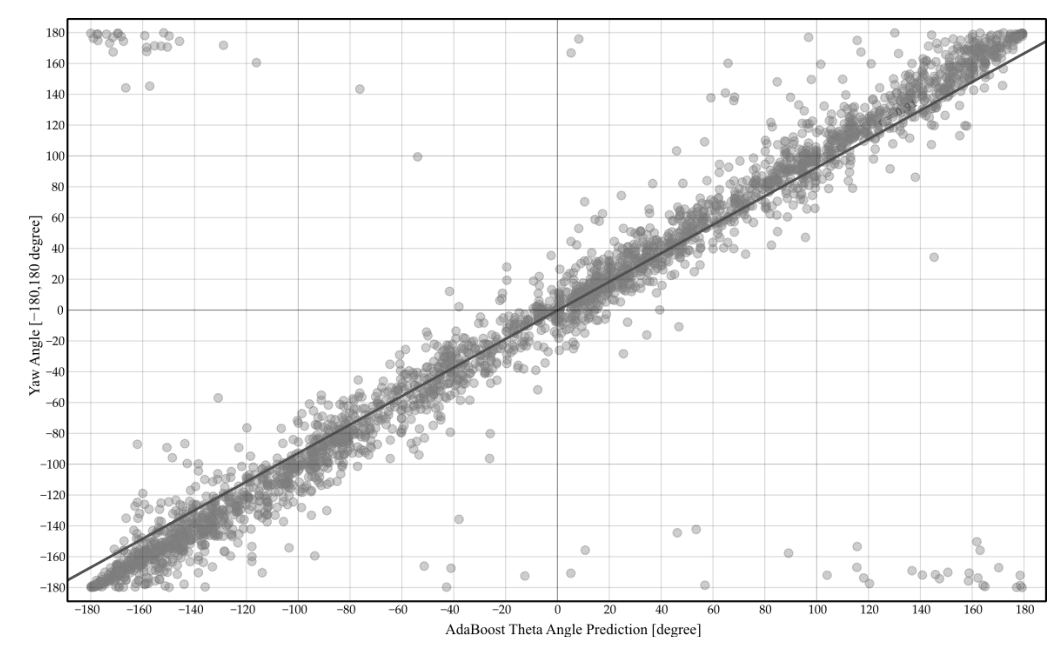
Autonomous robotic systems are increasingly being used not only outdoors but also indoors. For this reason, the need for precise position determination indoors as well as outdoors has become a necessity with new technological developments. Various techniques are currently used for precise position determination or navigation of autonomous robotic devices indoors. In this paper, we present a design for the use of visual reference markers for positioning and accurate navigation of a drone using visual odometry in an indoor warehouse environment. Our aim is to evaluate the efficiency of machine learning algorithms to perform more accurate and affordable positioning and navigation faster in the visual odometry method, which is one of the developing positioning systems used in indoor environments. In the simulation environment, data were collected by following various routes, and the collected data were subjected to machine learning algorithms, then the performance of K-Nearest Neighbors, Adaptive Boosting, Random Forest, Support Vector Machine, Artificial Neural Networks-Multilayer Perceptron algorithms were compared. In order to select the most successful algorithm, the R2 metric was used, which could provide information about how well it predicted the route followed. Among the machine learning algorithms used, AdaBoost gave the highest R2 value with 0.991 on the x-axis, the highest R2 value with 0.976 on the y-axis, the highest R2 value with 0.979 on the z-axis, and the highest R2 value with 0.816 in theta angle. As can be seen from these values, highly correlated predictions are realized, and indoor location prediction can be made as the vehicle sees one or more of the markers. Having a high correlation coefficient, the AdaBoost algorithm’s MAE value is 0.105 on the x-axis, 0.109 on the y-axis, 0.014 on the z-axis, and 14.956 on the theta angle. These values are in cm. It has been observed that the proposed system is able to perform a high correlation and low error positioning and navigation process. In addition, the proposed system offers an important alternative due to its low cost and less infrastructure installation requirement compared to similar and competing alternatives. Of course, other indoor positioning systems will continue to evolve to provide more accurate and faster positioning. However, the use of machine learning algorithms has increased the accuracy of indoor navigation to reliable levels. The choice of which machine learning algorithm and which indoor positioning system should be preferred for commercial use is open to debate. With future studies, it is aimed to create a real environment model and apply visual markers to this model and perform positioning by flying with a real drone. For the results to be more compatible with the actual values, we will work on an IMU-assisted system in our next study since it is thought that the prediction results of the pose information with IMU-assisted prediction will provide a higher prediction rate. At the same time, studies will continue to add and optimize new machine learning algorithms. Our study will also contribute to further studies on the Theta pose angle.
Transferring the proposed method from the simulation environment to the physical environment is a future study subject. Two methods can be applied here. In the first method, it is possible to use the simulation data exactly by drawing an exact or very similar model of the warehouse and labeling it to coincide with the same points, that is, creating a digital twin in a way. The second method is to collect data by flying the aircraft from fixed points and to collect learning data from scratch and perform the whole model extraction process according to that location.
The designed system will be needed in large areas in real applications. The main purpose of the study is to perform instant positioning and rack inventory counting. Applying the proposed method to a larger area or smaller area is just a scaling problem. The system can be easily adapted for a larger warehouse. Only a larger area definition, more racks, more VFM placements, and more data collection are required.

Author Contributions

Conceptualization, M.E., A.Ç.S., A.Ö. and C.K.; methodology, M.E., A.Ç.S., A.Ö. and C.K.; software, M.E., A.Ç.S., A.Ö. and C.K.; validation, M.E., A.Ç.S., A.Ö. and C.K.; investigation, M.E., A.Ç.S., A.Ö. and C.K.; resources, M.E., A.Ç.S., A.Ö. and C.K.; writing—original draft preparation, M.E., A.Ç.S., A.Ö. and C.K.; writing—review and editing, M.E., A.Ç.S., A.Ö. and C.K.; visualization, M.E., A.Ç.S., A.Ö. and C.K.; supervision, A.Ç.S. and C.K.; project administration, C.K. All authors have read and agreed to the published version of the manuscript.

Funding

This research received no external funding.

Data Availability Statement

Data and simulation files will be shared upon request from the authors.

Acknowledgments

This study was carried out within the scope of the doctoral thesis named “Positioning System Design for Independent Moving Aircraft”. The study was supported by the project numbered 2020FEBE046. The authors thank Pamukkale University in Turkey.

Conflicts of Interest

The authors declare no conflict of interest.

References

  1. Shakhatreh, H.; Sawalmeh, A.H.; Al-Fuqaha, A.; Dou, Z.; Almaita, E.; Khalil, I.; Othman, N.S.; Khreishah, A.; Guizani, M. Unmanned Aerial Vehicles (UAVs): A Survey on Civil Applications and Key Research Challenges. IEEE Access 2019, 7, 48572–48634. [Google Scholar] [CrossRef]
  2. Ayamga, M.; Tekinerdogan, B.; Kassahun, A.; Rambaldi, G. Developing a Policy Framework for Adoption and Management of Drones for Agriculture in Africa. Technol. Anal. Strateg. Manag. 2021, 33, 970–987. [Google Scholar] [CrossRef]
  3. Ayamga, M.; Akaba, S.; Nyaaba, A.A. Multifaceted Applicability of Drones: A Review. Technol. Forecast. Soc. Chang. 2021, 167, 120677. [Google Scholar] [CrossRef]
  4. Gyagenda, N.; Hatilima, J.V.; Roth, H.; Zhmud, V. A Review of GNSS-Independent UAV Navigation Techniques. Robot. Auton. Syst. 2022, 152, 104069. [Google Scholar] [CrossRef]
  5. Borenstein, J.; Everett, H.R.; Feng, L.; Wehe, D. Mobile Robot Positioning: Sensors and Techniques. J. Robot. Syst. 1997, 14, 231–249. [Google Scholar] [CrossRef]
  6. Liu, H.; Darabi, H.; Banerjee, P.; Liu, J. Survey of Wireless Indoor Positioning Techniques and Systems. Syst. Man Cybern. Part C Appl. Rev. IEEE Trans. 2007, 37, 1067–1080. [Google Scholar] [CrossRef]
  7. Vásárhelyi, G.; Virágh, C.; Somorjai, G.; Tarcai, N.; Szorenyi, T.; Nepusz, T.; Vicsek, T. Outdoor Flocking and Formation Flight with Autonomous Aerial Robots. In Proceedings of the Intelligent Robots and Systems (IROS 2014), 2014 IEEE/RSJ International Conference, Chicago, IL, USA, 14–18 September 2014; IEEE: Piscataway Township, NJ, USA; pp. 3866–3873. [Google Scholar]
  8. Quintero, S.; Collins, G.E.; Hespanha, J.P. Others Flocking with Fixed-Wing UAVs for Distributed Sensing: A Stochastic Optimal Control Approach. In Proceedings of the American Control Conference (ACC), Washington, DC, USA, 17–19 June 2013; pp. 2025–2031. [Google Scholar]
  9. Mautz, R. Overview of Current Indoor Positioning Systems. Geod. Kartogr. 2009, 35, 18–22. [Google Scholar] [CrossRef]
  10. Mautz, R. Indoor Positioning Technologies. Habilitation Thesis, ETH Zurich, Department of Civil, Environmental and Geomatic Engineering, Institute of Geodesy and Photogrammetry, Zürich Switzerland, 2012. [Google Scholar]
  11. Stirling, T.; Roberts, J.; Zufferey, J.-C.; Floreano, D. Indoor Navigation with a Swarm of Flying Robots. In Proceedings of the Robotics and Automation (ICRA), 2012 IEEE International Conference, Saint Paul, MN, USA, 14–18 May 2012; IEEE: Piscataway Township, NJ, USA; pp. 4641–4647. [Google Scholar]
  12. Scaramuzza, D.; Achtelik, M.C.; Doitsidis, L.; Friedrich, F.; Kosmatopoulos, E.; Martinelli, A.; Achtelik, M.W.; Chli, M.; Chatzichristofis, S.; Kneip, L. Vision-Controlled Micro Flying Robots: From System Design to Autonomous Navigation and Mapping in GPS-Denied Environments. IEEE Robot. Autom. Mag. 2014, 21, 26–40. [Google Scholar] [CrossRef]
  13. Balamurugan, G.; Valarmathi, J.; Naidu, V.P.S. Survey on UAV Navigation in GPS Denied Environments. In Proceedings of the 2016 International Conference on Signal Processing, Communication, Power and Embedded System (SCOPES), Paralakhemundi, India, 3–5 October 2016; pp. 198–204. [Google Scholar]
  14. Lu, Y.; Xue, Z.; Xia, G.-S.; Zhang, L. A Survey on Vision-Based UAV Navigation. Geo-Spat. Inf. Sci. 2018, 21, 21–32. [Google Scholar] [CrossRef] [Green Version]
  15. Beard, R.W.; McLain, T.W.; Goodrich, M.A.; Anderson, E.P. Coordinated Target Assignment and Intercept for Unmanned Air Vehicles. Robot. Autom. IEEE Trans. 2002, 18, 911–922. [Google Scholar] [CrossRef]
  16. Chen, Y.-C.; Wang, Y.-T. Obstacle Avoidance and Role Assignment Algorithms for Robot Formation Control. In Proceedings of the Intelligent Robots and Systems, 2007. IROS 2007. IEEE/RSJ International Conference, San Diego, CA, USA, 29 October–2 November 2007; IEEE: Piscataway Township, NJ, USA; pp. 4201–4206. [Google Scholar]
  17. Toner, J.; Tu, Y. Flocks, Herds, and Schools: A Quantitative Theory of Flocking. Phys. Rev. E 1998, 58, 4828. [Google Scholar] [CrossRef] [Green Version]
  18. Parker, L.E. Path Planning and Motion Coordination in Multiple Mobile Robot Teams. Encycl. Complex. Syst. Sci. 2009, 5783–5800. [Google Scholar]
  19. Jimenez, A.R.; Seco, F.; Prieto, C.; Guevara, J. A Comparison of Pedestrian Dead-Reckoning Algorithms Using a Low-Cost MEMS IMU. In Proceedings of the 2009 IEEE International Symposium on Intelligent Signal Processing, Budapest, Hungary, 26–28 August 2009; pp. 37–42. [Google Scholar]
  20. Do, T.-N.; Liu, R.; Yuen, C.; Zhang, M.; Tan, U.-X. Personal Dead Reckoning Using IMU Mounted on Upper Torso and Inverted Pendulum Model. IEEE Sens. J. 2016, 16, 7600–7608. [Google Scholar] [CrossRef]
  21. Brossard, M.; Barrau, A.; Bonnabel, S. AI-IMU Dead-Reckoning. IEEE Trans. Intell. Veh. 2020, 5, 585–595. [Google Scholar] [CrossRef]
  22. Durrant-Whyte, H.; Bailey, T. Simultaneous Localization and Mapping: Part I. IEEE Robot. Autom. Mag. 2006, 13, 99–110. [Google Scholar] [CrossRef] [Green Version]
  23. Thrun, S. Simultaneous Localization and Mapping. In Robotics and Cognitive Approaches to Spatial Mapping; Jefferies, M.E., Yeap, W.-K., Eds.; Springer Tracts in Advanced Robotics; Springer: Berlin/Heidelberg, Germany, 2008; pp. 13–41. ISBN 978-3-540-75388-9. [Google Scholar]
  24. Taheri, H.; Xia, Z.C. SLAM.; Definition and Evolution. Eng. Appl. Artif. Intell. 2021, 97, 104032. [Google Scholar] [CrossRef]
  25. Holmberg, M.; Karlsson, O.; Tulldahl, M. Lidar Positioning for Indoor Precision Navigation. In Proceedings of the IEEE/CVF Conference on Computer Vision and Pattern Recognition, Nashville, TN, USA, 20–25 June 2022; pp. 359–368. [Google Scholar]
  26. Seçkin, A.Ç. Pedestrian and Mobile Robot Detection with 2D LIDAR. EJOSAT 2021, 23, 583–588. [Google Scholar]
  27. Hess, W.; Kohler, D.; Rapp, H.; Andor, D. Real-Time Loop Closure in 2D LIDAR SLAM. In Proceedings of the 2016 IEEE International Conference on Robotics and Automation (ICRA), Stockholm, Sweden, 16–21 May 2016; pp. 1271–1278. [Google Scholar]
  28. Quan, S.; Chen, J. AGV Localization Based on Odometry and LiDAR. In Proceedings of the 2019 2nd World Conference on Mechanical Engineering and Intelligent Manufacturing (WCMEIM), Shanghai, China, 22–24 November 2019; pp. 483–486. [Google Scholar]
  29. Veerannapeta, V. Low Power Indoor Robotic Vacuum Cleaner Using Sensors and SLAM. Int. Res. J. Innov. Eng. Technol. 2019, 3, 51. [Google Scholar]
  30. Xin, C.; Wu, G.; Zhang, C.; Chen, K.; Wang, J.; Wang, X. Research on Indoor Navigation System of Uav Based on Lidar. In Proceedings of the 2020 12th International Conference on Measuring Technology and Mechatronics Automation (ICMTMA), Phuket, Thailand, 28–29 February 2020; pp. 763–766. [Google Scholar]
  31. Gümüşboğa, İ. İnsansız Hava Aracı Temelli Bir Otomatikleştirilmiş Stok Sayım Sistemi Tasarımı. Gazi Üniversitesi Mühendis. Mimar. Fakültesi Derg. 2022, 37, 1767–1782. [Google Scholar]
  32. Beinschob, P.; Reinke, C. Graph SLAM Based Mapping for AGV Localization in Large-Scale Warehouses. In Proceedings of the 2015 IEEE International Conference on Intelligent Computer Communication and Processing (ICCP), Cluj-Napoca, Romania, 3–5 September 2015; pp. 245–248. [Google Scholar]
  33. Chen, Y.; Wu, Y.; Xing, H. A Complete Solution for AGV SLAM Integrated with Navigation in Modern Warehouse Environment. In Proceedings of the 2017 Chinese Automation Congress (CAC), Jinan, China, 20–22 October 2017; pp. 6418–6423. [Google Scholar]
  34. Moshayedi, A.J.; Jinsong, L.; Liao, L. AGV (Automated Guided Vehicle) Robot: Mission and Obstacles in Design and Performance. J. Simul. Anal. Nov. Technol. Mech. Eng. 2019, 12, 5–18. [Google Scholar]
  35. Wang, H.; Wang, C.; Chen, C.-L.; Xie, L. F-Loam: Fast Lidar Odometry and Mapping. In Proceedings of the 2021 IEEE/RSJ International Conference on Intelligent Robots and Systems (IROS), Prague, Czech Republic, 27 September–1 October 2021; pp. 4390–4396. [Google Scholar]
  36. Gokula Vishnu Kirti, D.; Greesh Pranav, J.B.; Siva Naga Yaswanth, V.; Ponaka, A.R.; Arockia Dhanraj, J. Design and Development of Smart Multipurpose Automated Guided Vehicle Implemented with SLAM and AMCL. In Technology Innovation in Mechanical Engineering; Springer: Berlin/Heidelberg, Germany, 2022; pp. 469–481. [Google Scholar]
  37. Yazici, A.; Yayan, U.; Yücel, H. An Ultrasonic Based Indoor Positioning System. In Proceedings of the 2011 International Symposium on Innovations in Intelligent Systems and Applications, Istanbul, Turkey, 15–18 June 2011; pp. 585–589. [Google Scholar]
  38. Ijaz, F.; Yang, H.K.; Ahmad, A.W.; Lee, C. Indoor Positioning: A Review of Indoor Ultrasonic Positioning Systems. In Proceedings of the 2013 15th International Conference on Advanced Communications Technology (ICACT), PyeongChang, Republic of Korea, 27–30 January 2013; pp. 1146–1150. [Google Scholar]
  39. Seçkin, A.Ç.; Coşkun, A. Hierarchical Fusion of Machine Learning Algorithms in Indoor Positioning and Localization. Appl. Sci. 2019, 9, 3665. [Google Scholar] [CrossRef] [Green Version]
  40. Alitaleshi, A.; Jazayeriy, H.; Kazemitabar, S.J. WiFi Fingerprinting Based Floor Detection with Hierarchical Extreme Learning Machine. In Proceedings of the 2020 10th International Conference on Computer and Knowledge Engineering (ICCKE), Mashhad, Iran, 29–30 October 2020; pp. 113–117. [Google Scholar]
  41. Yamada, I.; Ohtsuki, T.; Hisanaga, T.; Zheng, L. An Indoor Position Estimation Method by Maximum Likelihood Algorithm Using RSS. In Proceedings of the SICE Annual Conference 2007, Takamatsu, Japan, 17–20 September 2007; pp. 2927–2930. [Google Scholar]
  42. Bahl, P.; Padmanabhan, V.N. RADAR: An in-Building RF-Based User Location and Tracking System. In Proceedings of the Proceedings IEEE INFOCOM 2000. Conference on Computer Communications. Nineteenth Annual Joint Conference of the IEEE Computer and Communications Societies (Cat. No.00CH37064), Tel Aviv, Israel, 26–30 March 2000; Volume 2, pp. 775–784. [Google Scholar]
  43. Mogi, T.; Ohtsuki, T. TOA Localization Using RSS Weight with Path Loss Exponents Estimation in NLOS Environments. In Proceedings of the 2008 14th Asia-Pacific Conference on Communications, Akihabara, Japan, 14–16 October 2008; pp. 1–5. [Google Scholar]
  44. Chan, Y.-T.; Tsui, W.-Y.; So, H.-C.; Ching, P. Time-of-Arrival Based Localization under NLOS Conditions. IEEE Trans. Veh. Technol. 2006, 55, 17–24. [Google Scholar] [CrossRef]
  45. Yamashita, J.; Hiyama, A.; Amemiya, T.; Kobayashi, I.; Hirota, K.; Hirose, M. Construction of outdoor virtual research environment for wearable and mobile computers. Hum. Interface Soc. 2002, 4, 45–48. [Google Scholar]
  46. Kushleyev, A.; Mellinger, D.; Powers, C.; Kumar, V. Towards a Swarm of Agile Micro Quadrotors. Auton. Robots 2013, 35, 287–300. [Google Scholar] [CrossRef]
  47. Leica TS30. Available online: http://www.leica-geosystems.us/downloads123/zz/tps/TS30/brochures/TS30_Brochure_us.pdf (accessed on 20 September 2022).
  48. Vicon MX Systems. Available online: http://www.vicon.com/products (accessed on 12 September 2022).
  49. Geiger, A.; Lenz, P.; Stiller, C.; Urtasun, R. Vision Meets Robotics: The Kitti Dataset. Int. J. Robot. Res. 2013, 32, 1231–1237. [Google Scholar] [CrossRef] [Green Version]
  50. Aqel, M.O.; Marhaban, M.H.; Saripan, M.I.; Ismail, N.B. Review of Visual Odometry: Types, Approaches, Challenges, and Applications. SpringerPlus 2016, 5, 1897. [Google Scholar] [CrossRef]
  51. Tiemann, J.; Wietfeld, C. Scalable and Precise Multi-UAV Indoor Navigation Using TDOA-Based UWB Localization. In Proceedings of the 2017 International Conference on Indoor Positioning and Indoor Navigation (IPIN), Sapporo, Japan, 18–21 September 2017; pp. 1–7. [Google Scholar]
  52. Cheng, Y.; Zhou, T. UWB Indoor Positioning Algorithm Based on TDOA Technology. In Proceedings of the 2019 10th International Conference on Information Technology in Medicine and Education (ITME), Qingdao, China, 23–25 August 2019; pp. 777–782. [Google Scholar]
  53. Zhu, X.; Yi, J.; Cheng, J.; He, L. Adapted Error Map Based Mobile Robot UWB Indoor Positioning. IEEE Trans. Instrum. Meas. 2020, 69, 6336–6350. [Google Scholar] [CrossRef]
  54. Zakiev, A.; Tsoy, T.; Shabalina, K.; Magid, E.; Saha, S.K. Virtual Experiments on ArUco and AprilTag Systems Comparison for Fiducial Marker Rotation Resistance under Noisy Sensory Data. In Proceedings of the 2020 International Joint Conference on Neural Networks (IJCNN), Glasgow, UK, 19–24 July 2020; pp. 1–6. [Google Scholar]
  55. Garrido-Jurado, S.; Muñoz-Salinas, R.; Madrid-Cuevas, F.J.; Marín-Jiménez, M.J. Automatic Generation and Detection of Highly Reliable Fiducial Markers under Occlusion. Pattern Recognit. 2014, 47, 2280–2292. [Google Scholar] [CrossRef]
  56. Nogar, S.M. Autonomous Landing of a UAV on a Moving Ground Vehicle in a GPS Denied Environment. In Proceedings of the 2020 IEEE International Symposium on Safety, Security, and Rescue Robotics (SSRR), Abu Dhabi, United Arab Emirates, 4–6 November 2020; pp. 77–83. [Google Scholar]
  57. Kato, H.; Billinghurst, M.; Poupyrev, I. ARToolKit Version 2.33. Hum. Interface Lab Univ. Wash. 2000, 2, 65. [Google Scholar]
  58. Wang, Y.; Zheng, Z.; Su, Z.; Yang, G.; Wang, Z.; Luo, Y. An Improved ArUco Marker for Monocular Vision Ranging. In Proceedings of the 2020 Chinese Control And Decision Conference (CCDC), Hefei, China, 22–24 August 2020; pp. 2915–2919. [Google Scholar]
  59. Masand, B.; Linoff, G.; Waltz, D. Classifying News Stories Using Memory Based Reasoning. In Proceedings of the 15th Annual International ACM SIGIR Conference on Research and Development in Information Retrieval, Copenhagen, Denmark, 21–24 June 1992; Association for Computing Machinery: New York, NY, USA, 1992; pp. 59–65. [Google Scholar]
  60. Altman, N.S. An Introduction to Kernel and Nearest-Neighbor Nonparametric Regression. Am. Stat. 1992, 46, 175–185. [Google Scholar] [CrossRef] [Green Version]
  61. Freund, Y.; Schapire, R.E. Experiments with a New Boosting Algorithm. In Machine Learning: Proceedings of the Thirteenth International Conference, Bari, Italy, 3–6 July 1996; Morgan Kaufmann Publishers Inc.: San Francisco, CA, USA, 1996; Volume 96, pp. 148–156. [Google Scholar]
  62. Freund, Y.; Schapire, R.E. A Decision-Theoretic Generalization of on-Line Learning and an Application to Boosting. J. Comput. Syst. Sci. 1997, 55, 119–139. [Google Scholar] [CrossRef] [Green Version]
  63. Bertoni, A.; Campadelli, P.; Parodi, M. A Boosting Algorithm for Regression. In Proceedings of the International Conference on Artificial Neural Networks, Lausanne, Switzerland, 8–10 October 1997; Springer: Berlin/Heidelberg, Germany, 1997; pp. 343–348. [Google Scholar]
  64. Breiman, L. Random Forests. Mach. Learn. 2001, 45, 5–32. [Google Scholar] [CrossRef] [Green Version]
  65. Liaw, A.; Wiener, M. Classification and Regression by RandomForest. R News 2002, 2, 18–22. [Google Scholar]
  66. Akman, M.; Genç, Y.; Ankarali, H. Random Forests Yöntemi ve Sağlık Alanında Bir Uygulama. Turk. Klin. J. Biostat. 2011, 3, 36–48. [Google Scholar]
  67. Adithya, V.; Deepak, G. HBlogRec: A Hybridized Cognitive Knowledge Scheme for Blog Recommendation Infusing XGBoosting and Semantic Intelligence. In Proceedings of the 2021 IEEE International Conference on Electronics, Computing and Communication Technologies (CONECCT), Bangalore, India, 9–11 July 2021; pp. 1–6. [Google Scholar]
  68. Da Silva, I.N.; Hernane Spatti, D.; Andrade Flauzino, R.; Liboni, L.H.B.; dos Reis Alves, S.F. Artificial Neural Networks; Springer International Publishing: Cham, Switzerland, 2017; ISBN 978-3-319-43161-1. [Google Scholar]
  69. Magree, D.; Johnson, E.N. Combined Laser and Vision-Aided Inertial Navigation for an Indoor Unmanned Aerial Vehicle. In Proceedings of the 2014 American Control Conference, Portland, OR, USA, 4–6 June 2014; pp. 1900–1905. [Google Scholar]
  70. Seçkin, A.Ç. Adaptive Positioning System Design Using AR Markers and Machine Learning for Mobile Robot. In Proceedings of the 2020 5th International Conference on Computer Science and Engineering (UBMK), Diyarbakir, Turkey, 9–11 September 2020; pp. 160–164. [Google Scholar]
  71. Marasigan, R.I.; Austria, Y.D.; Enriquez, J.B.; Lolong Lacatan, L.; Dellosa, R.M. Unmanned Aerial Vehicle Indoor Navigation Using Wi-Fi Trilateration. In Proceedings of the 2020 11th IEEE Control and System Graduate Research Colloquium (ICSGRC), Shah Alam, Malaysia, 8 August 2020; pp. 346–351. [Google Scholar]
  72. Khalaf-Allah, M. Particle Filtering for Three-Dimensional TDoA-Based Positioning Using Four Anchor Nodes. Sensors 2020, 20, 4516. [Google Scholar] [CrossRef] [PubMed]
  73. Alpaydin, E. Introduction to Machine Learning; MIT Press: Cambridge, MA, USA, 2009. [Google Scholar]
  74. Moriasi, D.N.; Arnold, J.G.; Van Liew, M.W.; Bingner, R.L.; Harmel, R.D.; Veith, T.L. Model Evaluation Guidelines for Systematic Quantification of Accuracy in Watershed Simulations. Trans. ASABE 2007, 50, 885–900. [Google Scholar] [CrossRef]
  75. Willmott, C.J. Some Comments on the Evaluation of Model Performance. Bull. Am. Meteorol. Soc. 1982, 63, 1309–1313. [Google Scholar] [CrossRef]
Figure 1. Indoor simulation environment images: (a) A view from y axis; (b) A view from x axis.
Drones 07 00003 g001
Figure 2. Common ArUco Marker types [55].
Drones 07 00003 g002
Figure 3. ArUco marker detection.
Drones 07 00003 g003
Figure 4. Instant positioning system with machine learning and visual reference markers.
Drones 07 00003 g004
Figure 5. Inventory counting program flowchart.
Drones 07 00003 g005
Figure 6. Inventory counting process steps screenshots: (a) Detection of ArUco within the warehouse area; (b) Rack mask extraction to scale by ArUco size; (c) AND operation of raw color image with mask; (d) Converting the image to gray scale; (e) Making a binary image with threshold adjustment; (f) Blurring the image; (g) Morphological gap closure; (h) Bitwise inversion of the image and bubble detection.
Drones 07 00003 g006
Figure 7. X-Axis prediction with AdaBoost.
Drones 07 00003 g007
Figure 8. Y-Axis prediction with AdaBoost.
Drones 07 00003 g008
Figure 9. Z-Axis prediction with AdaBoost.
Drones 07 00003 g009
Figure 10. Theta angular pose prediction with AdaBoost.
Drones 07 00003 g010
Figure 11. Detection of ArUco Marker by the camera and obtaining the necessary data for positioning the drone: (a) Detection of ArUco from drone camera while traversing on the X-axis; (b) Detection of ArUco from drone camera while traversing on the Y-axis; (c) Detection of ArUco from drone camera while traversing on the Z-axis; (d) ArUco detection from the camera of the drone with theta declination angle.
Drones 07 00003 g011
Table 1. Performance metrics for regression.
MetricEquation
Mean Absolute Error (MAE) MAE = 1 n j = 1 n | y j y ^ j |
R Coefficient of Determination (R-Square, R²) R 2 = 1 j = 1 n ( y j y ^ j ) 2 j = 1 n ( y j y ¯ ) 2
Table 2. X-axis machine learning performance.
ModelTime [s]Regression Metric
TrainTestMAER2
AdaBoost 20.4410.2580.1050.991
MLP 31.1930.0800.2300.983
K-NN 0.1050.6320.2370.976
RF 1.4200.0440.2390.974
XGBoost 1.3250.0270.3830.966
Table 3. Y-axis machine learning performance.
ModelTime [s]Regression Metric
TrainTestMAER2
AdaBoost 20.4020.2520.1090.976
MLP 50.2230.0730.2000.973
K-NN 0.1020.6060.2320.953
RF 1.4550.0350.2340.956
XGBoost 1.2930.0200.3280.946
Table 4. Z-axis machine learning performance.
ModelTime [s]Regression Metric
TrainTestMAER2
AdaBoost 23.7240.2530.0140.979
MLP 33.0420.0660.0620.968
K-NN 1.3060.0190.0470.966
RF 3.6540.0930.0380.964
XGBoost 0.1050.6500.0960.795
Table 5. Theta angular pose prediction machine learning performance.
ModelTime [s]Regression Metric
TrainTestMAER2
AdaBoost 15.6050.21414.9560.816
RF 01.2810.03519.6160.814
XGBoost 01.4270.02022.7310.810
MLP 39.6490.06722.6420.783
K-NN 00.1120.59322.2130.762
Table 6. Comparison of errors made by various systems according to the drone’s task dimensions.
ReferencePositioning MethodTask Dimensions (m)Task Area (m2)Minimum Error in x or y Axis (cm)Error (m)/Task Area (m2)
x Axisy Axisz Axis
[70]ArUco 0.801.00-0.80000.890.011125
[31]UWB4.754.362.6620.71000.260.000126
[72]UWB10.0010.0010.00100.000011.000.001100
[71]Wi-Fi15.2415.24-232.257643.000.001851
[69]Computer Vision and IMU3.653.65-13.322530.000.022518
[51]UWB1.803.60-6.48004.000.006173
Proposed MethodArUco and IMU10.0015.005.00150.000015.200.001013
Disclaimer/Publisher’s Note: The statements, opinions and data contained in all publications are solely those of the individual author(s) and contributor(s) and not of MDPI and/or the editor(s). MDPI and/or the editor(s) disclaim responsibility for any injury to people or property resulting from any ideas, methods, instructions or products referred to in the content.

