Article

Robust Control Strategy for Quadrotor Drone Using Reference Model-Based Deep Deterministic Policy Gradient

1
Graduate School of Science and Engineering, Chiba University, Chiba 263-8522, Japan
2
Jiangsu Collaborative Innovation Center of Atmospheric Environment and Equipment Technology (CICAEET), Nanjing University of Information Science & Technology, Nanjing 210044, China
*
Author to whom correspondence should be addressed.
Drones 2022, 6(9), 251; https://doi.org/10.3390/drones6090251
Submission received: 25 July 2022 / Revised: 7 September 2022 / Accepted: 8 September 2022 / Published: 12 September 2022
(This article belongs to the Special Issue Conceptual Design, Modeling, and Control Strategies of Drones-II)

Abstract

:
Due to the differences between simulations and the real world, the application of reinforcement learning (RL) in drone control encounters problems such as oscillations and instability. This study proposes a control strategy for quadrotor drones using a reference model (RM) based on deep RL. Unlike the conventional studies associated with optimal and adaptive control, this method uses a deep neural network to design a flight controller for quadrotor drones, which can map the drone’s states and target values to control commands directly. The method was developed based on a deep deterministic policy gradient (DDPG) algorithm combined with the deep neural network. The RM was further employed for the actor–critic structure to enhance the robustness and dynamic stability. The RM–DDPG-based flight-control strategy was confirmed to be practicable through a two-fold experiment. First, a quadrotor drone model was constructed based on an actual drone, and the offline policy was trained on it. The performance of the policy was evaluated via simulations while confirming the transition of system states and the output of the controller. The proposed strategy can eliminate oscillations and steady error and can achieve robust results for the target value and external interference.

1. Introduction

Unmanned aerial vehicles (UAVs), which have great potential for military, industrial, and civilian applications, have garnered significant attention in the last decade. The quadrotor drone is a type of UAV that was originally designed for military operations, but that was deemed unsuitable and/or dangerous to personnel. Recently, it has received increasing attention for its simple structure and small volume. After decades of development, quadrotor drones are being deployed in civilian fields such as delivery services [1], power line patrols [2], and agricultural services [3].

1.1. Related Work

The quadrotor drone, a classic type of UAV, has two pairs of propellers at diagonally opposite ends. One pair of propellers rotates clockwise while the other rotates counterclockwise. This ingenious design allows the quadrotor to realize vertical take-offs and landings, hovering, and other maneuvers. However, it moves nonlinearly and has an under-actuated system. Its design is not aerodynamically efficient and its propellers generate a small lift. Furthermore, quadrotor drones usually employ microelectromechanical systems as motion sensors. These sensors cannot accurately measure the states and parameters of drones, owing to the vibration of the propellers and airflow. Researchers have explored and proposed several effective control theories to overcome these challenges.
A proportional–integral–derivative (PID) controller has a simple form and is used in control systems such as servo systems, temperature control systems, and drones. However, the parameters of a PID controller are subjectively chosen based on experience. Therefore, its performance depends on the level of expertise. In scenarios where the system is more complex or has more requirements, the number of PID parameters can be large and interdependent, rendering them difficult to optimize or causing the controller to fail. Several model-based control methods were proposed to solve this challenge and improve the controller’s performance. The effectiveness of the linear–quadratic (LQ) optimal control algorithm [4] in controlling a nonlinear system by linearizing it within a certain range has been proven. However, linearization cannot be ensured if the system state changes beyond this range. Hence, the controller might perform worse when the drone is flying with high mobility. The application of model predictive control (MPC) [5,6] is becoming common in the control of complex systems such as robots because it can deal with multiple inputs and outputs. With its robustness to model errors and capability of solving optimization problems, MPC is a powerful approach to controlling complex systems through model prediction and optimal action choosing, but the performance of MPC has a strong dependence on the accuracy of the system model, which can be difficult to guarantee in some environments. The robust finite-time stability (RFTS) and stabilization (RFTU) [7] proposed a Cauchy-like matrix inequality method to handle the nonlinear terms of the system, which caused inaccuracies in the mathematical model. Moreover, to enable drones to work in complex environments such as tunnels, Elmokadem et al. [8] developed a computationally light navigation algorithm to autonomously guide the vehicle through such environments. Other advanced control strategies, such as the sliding mode control (SMC) [9,10], can ensure convergence in finite time through a sliding surface and the estimation of the upper bound of disturbances. Moreover, in [11], the adaptive barrier function was employed to handle the uncertainties and input constrains in a non-singular terminal sliding mode control (TSMC) method. In addition, Hoang et al. [12] introduced an adaptive twisting sliding mode (ATSM) control method, which could adjust the control gain of the twisting control law to control the attitude of quadrotors in harsh conditions. It showed strong robustness against disturbances while being adaptable to parametric variations within a fixed-time convergence. These model-based methods solved many problems in several fields and further improved the performance of the controller. However, they suffered from system nonlinearity and faced complex and dynamic environments. Hence, they are not suitable for all drone types and working scenarios.
Artificial intelligence has been progressing rapidly over the past few decades. Its application has significantly advanced image processing, simultaneous localization and mapping, robot perception and control, and other fields. Reinforcement learning (RL) networks, with the principle of reward and punishment, can learn and improve themselves during interactions with the environment.
Differently from supervised learning, the key thought of RL is driving an agent to interact with the environment and improve it according to the accumulated reward from the environment. Watkins and Dayan [13] proposed Q-learning, a classical method to optimally solve Markov decision process (MDP) [14] problems. This method maintains a Q-table to record the value of actions in every state and updates the table according to the reward during MDPs. This value-based approach provides the foundational “reinforcement” concept, but it can only handle simple problems with limited and discrete states and actions. To solve this problem, a study [15] used the deterministic policy gradient (DPG) to generate actions according to the states. The actions were performed sequentially in an environment to obtain the accumulated reward and optimize the policy. Moreover, with the development of neural network technology in recent years, researchers found it to be a powerful approach to approximate the state–action value function in RL. A deep DPG (DDPG) [16], which combines DPG with a deep neural network, was proposed. Zhang et al. [17] demonstrated a model-based RL control method for a virtual reality satellite. Liu et al. [18] applied the method to an underwater vehicle.
Furthermore, some simplified optimization methods were proposed to make RL algorithms more practical. Long et al. [19] introduced a single-critic NN-based RL method. Han et al. [20] proposed a guided RL method using double replay memory. Wang et al. [21] used an integral compensator to eliminate the steady-state error of the DDPG method; however, it was an external method that did not solve the problem in the controller. We proposed to develop an off-policy RL method structure to improve the practicality of the art of methods.

1.2. Contributions

At present, most of the proposed RL control methods show good performance in virtual environments such as Atari games and the Open AI gym. Dooraki et al. [22] proposed a bio-inspired flight controller (BFC) based on the PPO algorithm; they introduced the jumping distribution (JD), controlled starting state (CSS), and time-dependent terminal state (TDTS) methods to enhance the PPO algorithm to control a quadrotor drone, without any knowledge about their dynamic model and mathematical or physical rules, and the experiment showed that BFC performed significantly better than the classical DDPG, TRPO, and PPO algorithms in the Gazebo simulation environment. This is an inspiring achievement, but controlling the flight of a quadrotor drone in a real environment can be critically different; the dynamic model of a drone is complex and nonlinear, and there are many constraints on the mechanical properties of the power system. These properties bring gigantic challenges to reinforcement learning-based control algorithms. Traditional model-free RL methods are frequently concerned about the accumulated rewards that an environment yields during the MDP, and the rewards only depend on the errors. Even worse, a controller that is approximated by a neural network can choose the maximum action to reduce errors as soon as possible, regardless of the mechanical property constraints. By aiming at this problem, and compared with the proposed methods, the contributions of this paper are summarized as follows:
(1)
The method was to track the states of the reference model, which was designed according to a real system model. The reference mode can be seen as a baseline of actions to better direct the agent control quadrotor.
(2)
A reward-calculating system based on a model of a real quadrotor drone was designed to train the RL agent. At the same time, since the physical meanings and units were different between the system state variables, several hyperparameters were employed to adjust the weights of the state errors in the reward.
(3)
An RL-based quadrotor control algorithm, RM–DDPG, was proposed to improve the implementation performance, which can eliminate the steady-state error, reduce controller saturation, and guarantee robustness. To the best of our knowledge, this is the first time that the RL method has been applied to control a system with fast dynamics, such as a quadrotor attitude system, and this is the first experiment to demonstrate practical performance using an actual quadrotor drone.
The rest of the content of this paper is organized as follows. In Section 2, the dynamic model of the quadrotor drone is analyzed and given; then, the policy gradient is calculated, and the RM–DDPG algorithm is developed. In Section 3, the quadrotor model is verified, and the results and details of the experiment are given and discussed. The conclusion and further research goals are given in Section 4.

2. Problem Formulation

2.1. Dynamic Model of the Quadrotor Drone

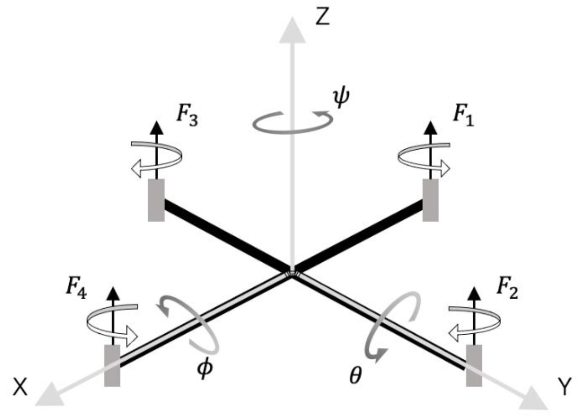
Referring to the Newton–Euler formalism, an intact structure of the quadrotor drone and its body-fixed frame is illustrated in Figure 1. We defined an earth-fixed frame on earth and a body-fixed frame at the center of the drone to demonstrate the translation and rotation of the quadrotor drone [23], respectively. Notably, the two coordinate systems were coincident initially; however, during the flight, they diverged. In this process, the earth-fixed frame remained unchanged, but the body-fixed frame moved and rotated. The translation from the earth-fixed frame to the body-fixed frame was assumed to be the position of the drone defined by P = x ,   y ,   z T . Its first and second derivatives P ˙ and P ¨ indicated the speed and dynamic acceleration of the drone, respectively. In the body-fixed frame, a set of Euler angles , φ , and ψ denoted the rotation about the x-, y-, and z-axes of the drone, respectively.
As illustrated in Figure 1, four rotors were fixed on the four ends of the cruciform frame of the quadrotor. L gives the half distance between the rotors on the diagonals. When viewed from above, the rotors in front (No. 4) and back (No. 1) spun counterclockwise, while those on the left (No. 2) and right (No. 3) spun clockwise. We controlled the rotation speeds of the four rotors individually by transmitting pulse-width modulation (PWM) signals to an electronic speed controller (ESC) separately. Furthermore, the rotation speed was almost proportional to the duty cycle of the PWM signal:
F i = K u i , i = 1 ,   2 ,   3 ,   4 ,  
where F i   i = 1 ,   2 ,   3 ,   4 is the thrust generated by the rotors, K is the speed gain of the PWM signal, and u i   i = 1 ,   2 ,   3 ,   4 repesents the normalized controller’s output, which ranged between 0 and 1 depending on the ratio of the rotation speed to the maximum speed. From a dynamic perspective, the difference in thrust between the propellers produced a rotational motion of the drone, and the total thrust of the four rotors and the attitude angle of the drone produced a translation motion. We analyzed the dynamic characteristics and applied Euler’s rotation equations to the body-fixed frame; the equation of the model of the quadrotor drone is:
M = M τ + M c + M f = I ω ˙ + ω × I ω ,
where ω = ϕ ˙ ,   θ ˙ ,   ψ ˙ T indicates the angular rate about the x-, y-, and z-axes of the body-fixed frame, respectively. I = d i a g I x ,   I y ,   I z is the drone’s diagonal form of an inertial matrix. M is the sum of the thrusts generated by the rotors. M τ = τ ϕ ,   τ θ ,   τ ψ T is the rotational moment due to the differences between the lift thrusts:
M τ = τ ϕ τ θ τ ψ = L T 2 T 3 L T 1 T 4 K ψ T 2 T 1 + T 3 T 4
In the body-fixed frame, τ θ and τ ϕ are the torques about the x- and y-axes, respectively. τ ψ is the control torque about the z-axis in the body-fixed frame, which was generally generated by the anti-torque force when the propellers rotated in the air. This torque was the lowest among the three torques; therefore, the rotational motion about the z-axis was the slowest. The reverse torque value was almost proportional to the lift thrust and is denoted by K ψ . The spinning rotors produced a gyroscope effect, represented by M c = I p θ ˙ Ω ,   I p ϕ ˙ Ω ,   0 T , where Ω is the disturbance effect of the propellers and I p is the moment of inertia. The rotational dynamic-drag torques are represented by M f = d ϕ ϕ ˙ , d θ θ ˙ , d ψ ψ ˙ T , where d ϕ , d θ , and d ψ are the rotational drag factors along the three axes, respectively.
In the earth-fixed coordinate frame, the translational motion model can be obtained from Newton’s second law:
F e = R F l + F d + G = m p ¨ ,  
where G is the gravitational force, F d is the aerodynamic drag, and F e indicates the resultant force of all external force vectors. F l = 0 ,   0 ,   F z denotes the sum of the thrusts generated by the rotors, where F z = i = 1 4 F i , with F i i = 1 ,   2 ,   3 ,   4 denoting the thrust generated by the four rotors, respectively. According to the standard motor installation method, the motor shaft should be parallel to the z-axis of the body-fixed coordinate. Therefore, the directions of the thrusts should always be same as the positive z-axis. Meanwhile, the velocity and position coordinates of the quadrotor are defined on the earth-fixed frame. We also introduce the transformation matrix R to transform the thrusts and torques from the body-fixed frame to the earth-fixed frame:
R = C ϕ C θ C ϕ S θ S ϕ C ϕ S ψ S ϕ S ψ + C ϕ C ψ S θ S ψ C θ S ϕ S θ S ψ + C ϕ C ψ C ϕ S θ S ψ C ψ S ϕ S θ C θ S ϕ C ϕ C θ ,  
where S · indicates sin ( · ), and C · indicates cos ( · ). d x , d y , and d z are the drag coefficients, and g is the acceleration due to gravity. Then, the aerodynamic drag will be F d = d x x ˙ ,   d y y ˙ ,   d z z ˙   T , and the gravitational force of drone G = 0 ,     0 , m g . T z denotes the resultant thrust from the four rotors. Finally, we obtained the nonlinear differential equations to express the quadrotor dynamics as follows:
ϕ ¨ = τ ϕ I p θ ˙ Ω d ϕ ϕ ˙ + θ ˙ ψ ˙ I y I z   /   I x
θ ¨ = τ θ I p ϕ ˙ Ω d θ θ ˙ + θ ˙ ψ ˙ I z I x   /   I y
ψ ¨ = τ ψ d ψ ψ ˙ + ϕ ˙ θ ˙ I x I y   /   I z
x ¨ = T z C ϕ S θ C ψ + S ϕ S ψ d x x ˙ / m
y ¨ = T z C ϕ S θ C ψ S ϕ S ψ d y y ˙ / m
z ¨ = T z C ϕ C θ d z z ˙ m g / m .
Due to the complexity of air dynamics and quadrotor components, some parameters of the model were unavailable to be measured directly. We had to utilize the model identification method to acquire the mathematical model, which was built and verified as described in Section 3.

2.2. Policy Gradient Method of Reinforcement Learning

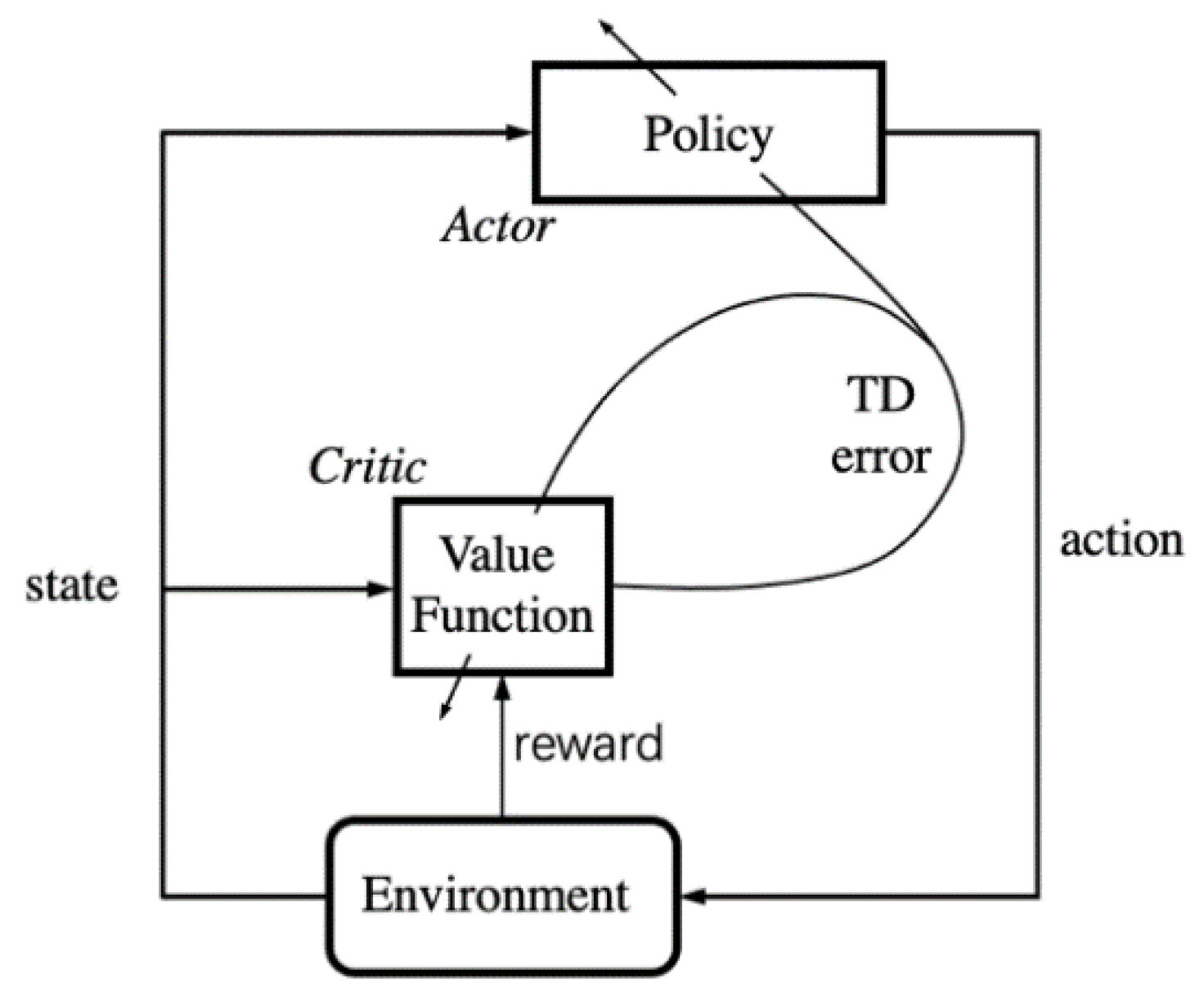
Figure 2 illustrates an agent–environment cyclic process. The agent, also called policy, can directly map situations to actions. The RL algorithm aims to optimize the policy by maximizing the accumulated rewards over the entire trajectory. Considering the formal framework of Markov decision processes (MDPs), with S as the set of states or observer of the system, in the proposed system, the states of the drone can be measured by sensors. Hence, this was a fully observable MDP. A represents the actions the agent can perform; they are real numbers in the quadrotor control problem. P denotes the state transition probability function, which depends on the quadrotor model and environment. R represents the reward function of the environment. Finally, the cyclic process can be formalized by a four-tuple ( S ,     A ,     P ,     R ).
If we suppose that the environment is in the state s t S at any timestep t, and it selects an action a t A according to the policy π , then the environment consequently transits to a new state s t + 1 S with a conditional probability P s t + 1 | s t ,   a t ) , simultaneously outputting a reward r t   ~   R s t ,   a t to the agent. As an MDP problem, the transitions must follow a stationary transition dynamic distribution with a conditional probability P ( s t + 1 | s 1 ,   a 1 ,   ,   s t ,   a t ) for each trajectory s 1 ,   a 1 ,   ,   s N ,   a N in the state–action space. For any timestep t, we defined the total discounted reward as the return R t = t = t N γ t t r t , and the discount factor γ 0 , 1 as a hyperparameter to control the weight of future rewards. For a trajectory starting from the timestep t, the expected return can be generally denoted as J π = E t = 1 N γ t 1 r t   |   π . The central optimization problem can then be expressed by π * = argmax π J π , where π * is the optimal policy. The action–value function Q π s t ,   a t = E π R t   |   s t ,   a t denotes the expected return that the agent starts in state s t , takes an arbitrary action a t (which may not have been obtained from the policy), and then infinitely executes actions following the policy π . It has been proven that all action–value functions obey the particularly consistent equation known as the Bellman expectation equation:
Q π s t , a t = E π R s t , a t + γ E a t + 1 ~ π Q π s t + 1 ,   a t + 1 .
Over the years, several practicable RL methods have been developed to optimize the policy, such as a policy gradient [24].
The main objective of the drone control problem is to find an optimal control policy, which can be used to drive the quadrotor in a fast and stable manner to the desired state. The policy gradient algorithm is an efficient way to solve this problem, as it can deal with continuous states and actions. In an environment with a state transition probability ρ , a parameterized stochastic policy π ϑ ( a | s ) can generate the control actions directly. Action a is executed with parameter ϑ while state s is given. Next, intuitively, the parameters can be adjusted by finding the gradient of the performance measurement J π ϑ . The gradient descent method can easily improve the policy. The principle of the policy gradient theorem is given as follows:
ϑ J π ϑ = E s ~ ρ π ϑ ,   a ~ π ϑ ϑ l o g π ϑ a | s Q π ϑ s , a | a = π ϑ s .
The policy gradient method demonstrates excellent performance in dealing with complex continuous problems. However, it suffers from two problems that severely limit its capabilities. The first problem is data efficiency. The full policy gradient can only be calculated after completing a trajectory. Once the parameters of the policy are optimized according to the calculated gradient, the trajectory data collected with the old policy will become useless. Then, the new policy can only be used to interact with the environment to generate trajectories and calculate the policy gradient. This reduces the efficiency of data utilization and extends the convergence time of the algorithm indefinitely. A more serious problem is that the stochastic policy generates actions through random sampling, which is impossible to predict and can be dangerous to actual drone control. Researchers have employed deterministic policies to improve this method, and these were used as the foundation of this study.

2.3. RM–DDPG Algorithm

The RM–DDPG algorithm was proposed based on the classical DDPG algorithm, which uses a deterministic policy to approximate the actor function instead of the stochastic policy in the original policy gradient method. In fact, the DDPG theory is a limiting case of the stochastic policy gradient theory.
The policy gradient method is perhaps the most advanced algorithm to deal with continuous-action problems using an RL algorithm. The basic idea of this algorithm is to use an actor function π μ to present the policy with the parameter μ , and then continually optimize the parameters μ along the direction of the performance gradient, given by:
μ J π μ = S   ρ π s A   μ π μ a | s Q π s , a d a d s = E s ~ ρ π   , a ~ π μ μ π μ s a Q π μ s , a ,
where Q π μ s , a is the action–value function. Notably, the distribution of state ρ π s depends on the parameters of the policy, and the policy gradient does not depend on the gradient of the state distribution.
The next issue to be solved is: how to estimate and evaluate the action–value function Q π s , a ? The actor–critic architecture has been widely used to solve this problem. In this architecture, the action–value function Q π s , a is replaced by another action–value function Q w s , a with parameter vector w, and a critic uses an appropriate policy evaluation method to estimate the action–value function Q w s , a Q π s , a . The off-policy deterministic actor–critic method is applied to update the parameters of the actor and critic function iteratively:
μ t + 1 = μ t + α μ μ π μ s t a Q w s t ,   a t |   a = π μ s
This is a parameter “soft” update method, where α μ is the updating rate, which can constrain the target values to change gradually, improving the learning stability. We also introduced a critic network to approximate the action–value function. Figure 3 illustrates this structure [20].
Using the Bellman equation, we improved the accuracy of the critic function by minimizing the difference between its two sides. Here, we define a temporal difference error (TD error):
δ t = r t + γ Q w s t + 1 ,   π μ s t + 1 Q w s t ,   a t  
The simple deterministic gradient decent policy to minimize the TD error is given by:
w t + 1 = w t + α w δ t w Q w s t ,   a t
As the quadrotor drone control is a complex nonlinear problem, the action and state spaces can be very large and continuous. It is generally difficult to estimate the actor function and action–value function (or critic function). Inspired by the DDPG algorithm, we used neural networks to approximate the policy and action–value function. Moreover, experience data replay [25] and target network methods were applied to improve the efficiency and stability of training.
Most optimization algorithms frequently assume that the samples of experimental data are independent and identically distributed; RL with neural networks is no exception. However, this assumption no longer holds true when samples are obtained during the continuous exploration of an environment. To address this issue, we used an M-sized replay buffer D = e 1 ,   e 2 ,   ,   e M to store the samples, where e = s t ,   a t ,   r t ,   s t + 1 denotes the transition experience data tuple of each timestep. The buffer works like a queue: its length is curtailed, and the oldest samples are dropped when the buffer becomes full. At each training episode, a miniature data batch is randomly sampled to update the actor and critic neural networks. Through this method, the associations between experimental data samples can be significantly reduced to satisfy the assumptions of independence and identical distribution. The efficiency of data and stabilization of training are improved. To further improve the learning stability, we designed target networks for both the actor and critic networks, similar to the target network used in [26]. However, we modified the networks for the actor–critic pair and only used a “soft” target update instead of directly copying the weights. Before the learning process commenced, the target network was created with parameters identical to those of the critic network. In each learning iteration, the weights of the target network were optimized first and then synchronized with the critic network through the “soft” update method, with an update rate η : w η w + 1 η w , where η 1 , and Q w s , a denotes the target critic network and w the weight of the network. As the changes in the target parameters are updated gradually, the learning process becomes more stable. This method moves the problem of learning the action–value function closer to supervised learning, such that a robust solution exists.
Next, we rewrote the updated equations of the target critic network using the experience replay method. During training, a batch of experience data tuples s i ,   a i ,   r i ,   s i , i = 1 ,   2 ,   ,   N were randomly sampled from the replay buffer. We minimized the loss function to update the critic network as follows:
L o s s w = 1 N i = 1 N y i Q w s i ,   a i 2
y i = r i + γ Q w s i + 1 ,   π μ s i
where y i is the output of the target critic network with the reward of action. The gradient decent method to update the critic network parameters is given as follows:
w L o s s w = 1 N i = 1 N y i Q w s i ,   a i w Q w s i ,   a i
w t + 1 = w t + α w w L o s s w
Meanwhile, we also updated the actor network parameters following the DDPG algorithm:
μ J μ = 1 N i = 1 N μ π μ s i a Q w s i ,   a i |   a i = π μ s i
μ t + 1 = μ t + α μ μ J μ
The DDPG algorithm has been proven to be an effective method to learn a stable and fast-responding policy for simulated control tasks in classic control and multi-joint dynamics with contact or MuJoCo environments of the open-source gym library. However, according to the results of the extensive experiments in this study, control saturation and steady-state error were two glaring challenges in the application of the DDPG algorithm with the neural network for quadrotor control.
Control saturation is a common problem among control algorithms for quadrotor control or any other motion control. Preferably, the controlled object must be able to respond to the target value at the earliest. This may fetch good results in simulation experiments; however, in practical application scenarios, a rapid response requires the support of strong hardware, which is generally unavailable. We examined this problem and marked reward as the key reason, according to Equations (18) and (19). While updating the critic network by minimizing the loss function, the reward was an important basis for each iteration. The reward obtained by the current TD error algorithm is a simple scalar quantity, such as attitude control of the quadrotor drone, which is the error between the target and feedback attitude angles. This strategy of receiving a reward may work well for simple control problems, such as CartPole. However, for complex tasks such as quadrotor drone control, the controlled object has several significant state quantities, such as the angle, angular velocity, and angular acceleration. The control goal of this study was not merely to track the attitude angle of the target at the earliest, but also to stabilize and safeguard the system. After introducing the reference model, we improved the reward function in the following manner:
r i = k = 1 n λ k R e f s k s k ,   k = 1 , 2 , , n ,  
where n represents the n-dimensional state variables in the controlled system, R e f s k denotes the reference states, s k is the state variable, and λ k is the weight set according to experience.
Regarding the steady-state error, the results of the experiments demonstrated that the learned controller in most scenarios cannot eliminate the tracking error, regardless of the time, type of training strategy, or a number of iterations provided to the controller. We offer two plausible reasons for this. As implied in [13], one reason can be inaccurate function estimation value. Owing to limited sampling, accurate values of the actions could not be obtained. The accurate estimation becomes more difficult for complex problems such as quadrotor drone control. The most important reason is that the policy, which was trained by the DDPG algorithm, is the optimal controller. It is not a servo system, as it does not consider the error integral; for systems with damping and external disturbances, a steady-state error cannot be eliminated by this method.
To design a control system for a quadrotor drone with excellent stability and dynamic performance, we designed a reference model to generate the reference signals according to the target and reanalyzed the quadrotor drone model. We formed the quadrotor drone model by selecting the angle, angular velocity, angular acceleration, and angle error integral as the state variables. The specified reference model, where the state variables directly correspond to the identified model, was constructed as:
x ˙ m = A m x m + B m u r
y m = C m x m
Here, u r is the reference input. If C m = C and e = x x m , the state variable error dynamics can be determined as follows:
e ˙ = A m e + A A m x + B u B m u r
To eliminate the steady-state error, a novel state ε y was introduced:
ε ˙ y = y y m
The expansion system is given as follows:
e ˙ s = e ˙ ε ˙ y = A m 0 C m 0 e ε y + B 0 u s = A s e s + B s u s  
In the end, we obtained a three-order reference model with the state variables of angular acceleration, angular velocity, and angle reference. The quadrotor model state variables were angular acceleration, angular velocity, integral of angle error, and angle. This standard servo system can remain stable and provide a rapid response.

2.4. Neural Network Structure

Contrary to the stochastic policy, the deterministic policy requires additional strategies instead of naturally exploring the state–action space. As presented in the previous section, we added Gaussian noise to the output actions to construct the exploration policy A ¯ s :
A ¯ s t = A μ s t + n t ,   n t ~ Ν 0 ,   σ 2
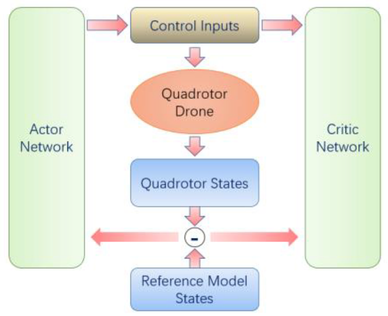
Figure 4 illustrates the structure of the RM–DDPG algorithm. The green module on the left is the actor network, which used the state θ ¨ ,   θ ˙ ,   θ and the reference model state R θ ¨ ,   R θ ˙ ,   R θ as the input.
Next, we considered the symmetry of the structure of the quadrotor drone. We used the same controller to control its roll and pitch. This network was designed following the procedure in [27], and the goal was to continuously approximate to an actor function that had the best control performance and stability. We also considered that the output of the actor network should be smooth. Hence, we designed it with two 128-dim fully connected hidden layers and a tanh activation function. The actor network triggered an action command that was relayed to the motor. In the control problem of a drone, the action command is also the action space of the RL algorithm. In practical applications, it is a continuous quantity in an interval and is limited to [−3 rad/s, 3 rad/s] by the mechanical properties of the drone. For practical purposes, to limit the control signals within a reasonable range, we also applied the tanh function to the output layer. The critic network is depicted on the right-hand side of Figure 4; the inputs were the quadrotor and reference model states, and the control inputs were generated by the actor network. Similar to the actor network, the output network also had two hidden layers and activation functions. However, the activation function was changed to a linear function to better approximate the action–value function. The center of Figure 4 illustrates the quadrotor drone model, which is given in Equation (28), and the steady-state error was introduced into the system as a state variable. The objective of this method was to ensure that the actor network considered the steady-state error when generating the control input, and more importantly, that the critic network considered the quadrotor state, the reference model state, and the steady-state error of the quadrotor states. While optimizing the critic network, the gradient policy changed this objective to keep the quadrotor states close to the reference model states, instead of fast-tracking to the target angle, which can lead to control saturation and the elimination of the steady-state error.
Next, we designed an algorithm in the episodic style. First, we created a target critic network with parameters identical to those of the critic network and generated the initial states within the prop range for each episode, following which the actor network relayed control commands to the quadrotor drone model. For each step, the transition of model states was temporarily stored in the replay buffer, and the training commenced if adequate samples were provided. Finally, the offline RL is summarized in Algorithm 1.
Algorithm 1 Offline training algorithm of RM–DDPG.
Initialize:
  Randomly initialize the weights of the actor network π μ and critic network Q w
  Copy parameters from the actor network π μ and critic network Q w to the target actor network π μ and target critic network Q w , respectively
  Create an empty replay buffer D with length M
  Load the quadrotor drone model and the reference model as the environment
  Create a noise distribution N(0, σ 2 ) for exploration
For episode = 1, M do
  Randomly reset quadrotor states and target states
  Initialize the reference model states by copying quadrotor states
  Observe initial states s 1
  For t = 1, T do
   If length of replay buffer D is bigger than mini-batch size, then
    Choose action a t = π μ s t + n t based on state s t and noise n t ~ N
   Else
    Choose an arbitrary action from the action space
   End if
   Perform control command a t in the environment
   Calculate reward r t and new state s t + 1
   Store transition tuple ( s t , a t , r t , s t + 1 ) to replay buffer D
   If the length of replay buffer D is bigger than mini-batch size, then
    Randomly sample a data batch from D
    Calculate the gradient and update the critic network following (20) (21)
    According to the output of the critic network, update the actor network -following (22) (23)
    Soft update the target network parameters following (18)
   End if
   If s t + 1 exceed the safe range then
     break
    End If
   End For
End For
 Save model or evaluate

3. Experiments and Analysis

In this section, we comprehensively evaluate the controller trained by the proposed approach. First, the details of the implementation and learning progress are presented, and subsequently, the control input was compared with DDPG. Finally, we used the well-trained controller on different drones with different dimensions to test the robustness of the model. The results demonstrated the robustness of the algorithm. It greatly inhibited control saturation and effectively eliminated the steady-state error.

3.1. Drone Model and Simulator

For the drone model, we selected a plant protection quadrotor drone with a brushless power system; the drone parameters are listed in Table 1. Next, we identified the dynamic model with the measured drone parameters. We tried several model types and parameters, and the second-order processing model without a delay fit the angular rate model of the quadrotor well. The model parameters were identified through sectional data, including prop frequency signals (Figure 5a); then, the model was verified on the whole flying data (Figure 5b). The ident tool gave an 80% similarity between the measured signal and model output, and the delay and amplitude differences in several signal frequencies were also within a narrow limit. For the convenience of simulation and RL training, we transformed the continuous transfer function model into a discrete state space model; the angular velocity response is illustrated in Figure 6.
According to the angular rate model and Equations (25) and (26), we extended the state space model to the third order and designed an attitude reference model that could acquire balance and stability and provide a fast response; the step response of this model is illustrated in Figure 7.
The simulator was constructed based on the previous section and was extended to the form of Equation (30). The experiments were run on an Ubuntu 16.04 operation system powered by AMD Ryzen 7 5800X @3.8GHz with eight cores, and with Nvidia 2080Ti GPU to accelerate the neural network computation. The neural networks and model simulation were developed with Python and Pytorch. The training parameters are listed in Table 2.
The training followed Algorithm 1 using RM–DDPG with the parameters in Table 2. Figure 8 illustrates the average accumulated reward in each training step.

3.2. Performance Test

To test the performance of the RL controller, we designed comparative experiments with classical DDPG and our method, through a step response and a sine wave response. Figure 9 illustrates the transition of the system states and control inputs of the two methods.
Figure 9a,b illustrates the step response and sine wave response of classical DDPG and RM–DDPG algorithms. As shown in the figure, the classical DDPG algorithm always tended to choose the maximum control input to track the target value; the tracking speed was very fast, such that it could drive the quadrotor to a 0.7 rad angle (about 40 degrees) in 0.25 s. This is a reasonable phenomenon; since the evaluation criterion of an actor neural network is the accumulated reward during the step response, the fastest tracking can achieve more reward. However, as a consequence, the control input was too strong, so that a little noise can lead to the oscillation of the system. Instead, the RM–DDPG responded based on changes in the reference model, finding a good balance between the stability and speed of the response. Furthermore, the process of neural network optimization cannot strictly guarantee global optimality, so the steady error cannot be eliminated. We designed an error integral section among the reward function and adjusted the weight to drive the RM–DDPG algorithm to eliminate steady errors.

3.3. Robustness Test

For the robustness test, we changed the diagonal length of the quadrotor drone to 0.8 m (30% smaller), 1.3 m (20% larger), and 1.5 m (40% larger) while maintaining a constant power system. Next, we applied the controller to drones of different sizes. Figure 10 displays the results of roll−angle control; the left graph demonstrates that the controller could propel different sizes of drones with a consistent performance. The right graph demonstrates that the controller accepted different control signals to maintain a consistent performance. Furthermore, we designed a test to determine if the RM–DDPG controller drives the quadrotor to return to the horizontal state from different initial angles. Figure 11 demonstrates that the controller could always drive the quadrotor to return to a stable state placidly.

3.4. Real Flight Experiment

As a consensus, there are many great differences from the simulation and a real environment. The mechanical properties, the noise of sensors, and external disturbances can lead to the distinct performance of the controller. To verify the performance of the classical DDPG method and our RM–DDPG method, we trained the two agents, one for each method, on the same quadrotor model and in an environment with the same hyperparameters. Figure 12 shows the performance of the two controllers; the classical DDPG kept the quadrotor roughly stable. However, when the target angle changed to not zero, due to the greedy characteristic of the classical DDPG algorithm to minimize errors as soon as possible, the controller took too radical of an action, which led to divergence rapidly in 3−5 s. On the other hand, our RM–DDPG method still maintained a stable performance in the actual flight experiment, since the target state variables were given by the reference model, which can generate a trajectory that conforms to the laws of the physical world and the power system capabilities of the drone. In general, this approach improved the stability by sacrificing the tracking speed, and the balance of these two metrics depended on the considerations when designing the reference model.

4. Discussion and Conclusions

With decades of development, immense progress has been made in RL, and its application range has expanded from simple binary games to dealing with complex problems such as continuous states and actions. However, RL has always been limited by the virtual environment, because it must interact with the latter to acquire experience data. When applied to drone control, RL encounters several problems, including control saturation and steady−state error, due to the differences between the virtual environment and the real world.
To solve these problems, we proposed a deep deterministic policy gradient for quadrotor control based on a reference model. We performed an in−depth analysis of the drone model and solved the problems by designing reference models and system state variables. The proposed algorithm successfully improved the stability of reinforcement control and eliminated the steady−state error. Notably, this study proposed an accessible and robust method for applying RL to practical quadrotor control. The simulation and actual flight experiment demonstrated that the RM–DDPG method performs with better stability and robustness than the classical DDPG method in the control of quadrotors.
For further research, an online training process requires powerful hardware, which may not fit the small form factor of a drone; hence, we had to train the network offline and then upload it to the drone. Although we constructed the drone model with the highest possible accuracy, the algorithm’s performance was limited by the difference between the simulated environment and the real world. Future research should utilize distributed training methods or downsize the network to reduce computations for the on−drone computer.

Author Contributions

Conceptualization, H.L. (Hongxun Liu); methodology, S.S. and W.W.; software, H.L. (Hongxun Liu); validation, H.L. (Hongxun Liu) and Q.W.; formal analysis, H.L. (Hongxun Liu); investigation, H.L. (Hongxun Liu); resources, S.S.; data curation, H.L. (Hongxun Liu); writing—original draft preparation, H.L. (Hongxun Liu); writing—review and editing, H.L. (Hao Liu); visualization, H.L. (Hongxun Liu); supervision, S.S. and W.W. All authors have read and agreed to the published version of the manuscript.

Funding

This research received no external funding.

Institutional Review Board Statement

Not applicable.

Informed Consent Statement

Not applicable.

Data Availability Statement

Not applicable.

Acknowledgments

The authors would like to thank the Graduate School of Science and Engineering, Chiba University, Chiba, Japan, for the resources provided by them.

Conflicts of Interest

The authors declare no conflict of interest.

References

  1. Eun, J.; Song, B.D.; Lee, S.; Lim, D.-E. Mathematical Investigation on the Sustainability of UAV Logistics. Sustainability 2019, 11, 5932. [Google Scholar] [CrossRef]
  2. An, C.; Mingxi, J.; Jieyin, N.; Zhou, W.; Li, X.; Wang, J.; He, X. Research on the application of computer track planning algorithm in UAV power line patrol system. J. Phys. Conf. Ser. 2021, 1915, 032030. [Google Scholar]
  3. Valente, J.; del Cerro, J.; Barrientos, A.; Sanz, D. Aerial coverage optimization in precision agriculture management: A musical harmony inspired approach. Comput. Electron. Agric. 2013, 99, 153–159. [Google Scholar] [CrossRef]
  4. Cowling, I.D.; Yakimenko, O.A.; Whidborne, J.F.; Cooke, A.K. A prototype of an autonomous controller for a quadrotor UAV. In Proceedings of the 2007 European Control Conference (ECC), Kos, Greece, 2–5 July 2007; pp. 4001–4008. [Google Scholar] [CrossRef]
  5. Camacho, E.F.; Alba, C.B. Model Predictive Control; Springer Science & Business Media: London, UK, 2013. [Google Scholar]
  6. Mayne, D.Q. Model predictive control: Recent developments and future promise. Automatica 2014, 50, 2967–2986. [Google Scholar] [CrossRef]
  7. Puangmalai, W.; Puangmalai, J.; Rojsiraphisal, T. Robust Finite-Time Control of Linear System with Non-Differentiable Time-Varying Delay. Symmetry 2020, 12, 680. [Google Scholar] [CrossRef]
  8. Elmokadem, T.; Savkin, V.A. A method for autonomous collision-free navigation of a quadrotor UAV in unknown tunnel-like environments. Robotica 2022, 40, 835–861. [Google Scholar] [CrossRef]
  9. Xu, R.; Ozguner, U. Sliding mode control of a quadrotor helicopter. In Proceedings of the 45th IEEE Conference on Decision and Control, San Diego, CA, USA, 13–15 December 2006; pp. 4957–4962. [Google Scholar] [CrossRef]
  10. Xu, B. Composite learning finite-time control with application to quadrotors. IEEE Trans. Syst. Man Cybern. Syst. 2018, 48, 1806–1815. [Google Scholar] [CrossRef]
  11. Alattas, K.A.; Vu, M.T.; Mofid, O.; El-Sousy, F.F.M.; Fekih, A.; Mobayen, S. Barrier Function-Based Nonsingular Finite-Time Tracker for Quadrotor UAVs Subject to Uncertainties and Input Constraints. Mathematics 2022, 10, 1659. [Google Scholar] [CrossRef]
  12. Hoang, V.T.; Phung, M.D.; Ha, Q.P. Adaptive twisting sliding mode control for quadrotor unmanned aerial vehicles. In Proceedings of the 2017 11th Asian Control Conference (ASCC), Gold Coast, QLD, Australia, 17–20 December 2017; pp. 671–676. [Google Scholar]
  13. Watkins, C.J.C.H. Learning from Delayed Rewards. Ph.D. Thesis, King’s College, Cambridge, UK, 1989. [Google Scholar]
  14. Watkins, C.J.C.H.; Dayan, P. Q-learning. Mach. Learn. 1992, 8, 279–292. [Google Scholar] [CrossRef]
  15. Silver, D.; Lever, G.; Heess, N.; Degris, T.; Wierstra, D.; Riedmiller, M. Deterministic policy gradient algorithms. In Proceedings of the 31st International Conference on Machine Learning, Beijing, China, 21–26 June 2014; pp. 387–395. [Google Scholar]
  16. Lillicrap, T.P.; Hunt, J.J.; Pritzel, A.; Heess, N.; Erez, T.; Tassa, Y.; Silver, D.; Wierstra, D. Continuous control with deep reinforcement learning. arXiv 2015, arXiv:1509.02971. [Google Scholar] [CrossRef]
  17. Zhang, J.; Wu, F. A novel model-based reinforcement learning attitude control method for virtual reality satellite. Wirel. Commun. Mob. Comput. 2021, 2021, 7331894. [Google Scholar] [CrossRef]
  18. Liu, T.; Hu, Y.; Xu, H. Deep reinforcement learning for vectored thruster autonomous underwater vehicle control. Complexity 2021, 2021, 6649625. [Google Scholar] [CrossRef]
  19. Long, X.; He, Z.; Wang, Z. Online optimal control of robotic systems with single critic NN-based reinforcement learning. Complexity 2021, 2021, 8839391. [Google Scholar] [CrossRef]
  20. Han, J.; Jo, K.; Lim, W.; Lee, Y.; Ko, K.; Sim, E.; Cho, J.S.; Kim, S.H. Reinforcement learning guided by double replay memory. J. Sens. 2021, 2021, 6652042. [Google Scholar] [CrossRef]
  21. Wang, Y.; Sun, J.; He, H.; Sun, C. Deterministic policy gradient with integral compensator for robust quadrotor control. IEEE Trans. Syst. Man Cybern. Syst. 2020, 50, 3713–3725. [Google Scholar] [CrossRef]
  22. Dooraki, A.R.; Lee, D.J. An innovative bio-inspired flight controller for quad-rotor drones: Quad-rotor drone learning to fly using reinforcement learning. Robot. Auton. Syst. 2021, 135, 103671. [Google Scholar] [CrossRef]
  23. Rozi, H.A.; Susanto, E.; Dwibawa, I.P. Quadrotor model with proportional derivative controller. In Proceedings of the 2017 International Conference on Control, Electronics, Renewable Energy and Communications (ICCREC), Yogyakarta, Indonesia, 26–28 September 2017; pp. 241–246. [Google Scholar] [CrossRef]
  24. Sutton, R.S.; McAllester, D.; Singh, S.; Mansour, Y. Policy gradient methods for reinforcement learning with function approximation. Adv. Neural Inf. Process. Syst. 1999, 12, 1057–1063. [Google Scholar]
  25. Lin, L.-J. Reinforcement Learning for Robots Using Neural Networks. Ph.D. Thesis, Carnegie Mellon University, Pittsburgh, PA, USA, 1993. [Google Scholar]
  26. Mnih, V.; Kavukcuoglu, K.; Silver, D.; Graves, A.; Antonoglou, I.; Wierstra, D.; Riedmiller, M. Playing Atari with deep reinforcement learning. arXiv 2013, arXiv:1312.5602. [Google Scholar] [CrossRef]
  27. Hwangbo, J.; Sa, I.; Siegwart, R.; Hutter, M. Control of a quadrotor with reinforcement learning. IEEE Robot. Autom. Lett. 2017, 2, 2096–2103. [Google Scholar] [CrossRef] [Green Version]
Figure 1. Coordinate system of the quadrotor drone.
Drones 06 00251 g001
Figure 2. Agent–environment cyclic process.
Drones 06 00251 g002
Figure 3. Actor–critic structure.
Drones 06 00251 g003
Figure 4. The network structure of the RM–DDPG algorithm.
Drones 06 00251 g004
Figure 5. (a) The angular rate model of the quadrotor was identified through sectional data; (b) shows the fitting result on the whole flying data. Considering the safety of the experiment, the time of the data did not start from 0 s.
Drones 06 00251 g005
Figure 6. (a) Step response of the angular velocity model, and (b) extension of the attitude angle. The SI units on the x− and y−axes are s and rad/s, respectively. As this is the step response of the angular velocity, the angle in (b) is in the shape of a ramp.
Drones 06 00251 g006
Figure 7. (a) Step response of the designed reference model. (b) The x−axis represents the time (s), and the y−axis represents the target angle, angular velocity, and angular acceleration in rad, rad/s, and rad/ s 2 .
Drones 06 00251 g007
Figure 8. Average accumulated reward in each training step.
Drones 06 00251 g008
Figure 9. The transition of system states (angle, angular rate) and control input during the step response (a) and sine wave response (b). The maximum control input was 3.0. It can be seen that classical DDPG tended to provide the maximum control input, which was unacceptable to a real quadrotor. By contrast, RM–DDPG was softer and could significantly eliminate steady−state errors.
Drones 06 00251 g009
Figure 10. Performance of the controller in drones with different diagonal lengths. The controller implemented the control policy corresponding to the size of the drone to maintain a consistent attitude control performance. (a) The attitude angle during the step response of drones with different diagonal lengths; (b) control input during the step response of drones with different diagonal lengths.
Drones 06 00251 g010
Figure 11. RM–DDPG method drove the quadrotor to return to the stable status from different initial angles.
Drones 06 00251 g011
Figure 12. Experimental results on a real quadrotor. (a) Flight experiment of classical DDPG on a real quadrotor drone; (b) flight experiment of our RM–DDPG on the same real quadrotor drone.
Drones 06 00251 g012
Table 1. Parameters of the drone.
ParameterDescriptionValue
LDiagonal length1.1 (m)
mTake-off weight6.8 (kg)
gAcceleration due to gravity 9.81   ( m / s 2 )
KThrust gain9.01
I x , I y , I z Moments of inertia of frame 0.04 ,   0.04 ,   0.05   ( kg · m 2 )
J p Moments of inertia of proper 0.00007   ( kg · m 2 )
Table 2. Parameters of training.
ParameterValue
Learning rate of critic network α w 0.001
Learning rate of actor network α μ 0.003
Batch size N256
Replay buffer size M100,000
Discount factor γ 0.99
Soft update rate η 0.002
Noise variance σ 0.1
Simulation timestep0.02 (s)
Maximum steps in an episode500
Publisher’s Note: MDPI stays neutral with regard to jurisdictional claims in published maps and institutional affiliations.

