Thermal and Visual Tracking of Photovoltaic Plants for Autonomous UAV Inspection

Abstract

Because photovoltaic (PV) plants require periodic maintenance, using unmanned aerial vehicles (UAV) for inspections can help reduce costs. Usually, the thermal and visual inspection of PV installations works as follows. A UAV equipped with a global positioning system (GPS) receiver is assigned a flight zone, which the UAV will cover back and forth to collect images to be subsequently composed in an orthomosaic. When doing this, the UAV typically flies at a height above the ground that is appropriate to ensure that images overlap even in the presence of GPS positioning errors. However, this approach has two limitations. First, it requires covering the whole flight zone, including “empty” areas between PV module rows. Second, flying high above the ground limits the resolution of the images to be subsequently inspected. The article proposes a novel approach using an autonomous UAV with an RGB and a thermal camera for PV module tracking through segmentation and visual servoing, which does not require a GPS except for measuring the “small” relative displacement between a PV module row and the next one. With this solution, the UAV moves along PV module rows at a lower height than usual and inspects them back and forth in a boustrophedon way by ignoring “empty” areas with no PV modules. Experimental tests performed in simulation and at an actual PV plant are reported, showing a tracking error lower than 0.2 m in most situations when moving at 1.2 m/s.

1. Introduction

We are currently facing a worldwide energy challenge that requires us to search for alternatives to fossil fuels, including green and renewable energies [1]. According to [2], in 2019, renewable energy sources made up 34% of gross electricity consumption in the EU-27, slightly up from 32% in 2018. While wind and hydropower accounted for two-thirds of the total electricity generated from renewable sources (35% each), the remaining one-third of the electricity generated was from solar power (13%), solid biofuels (8%), and other renewable sources (9%). The analysis also shows how solar power is the renewable source experiencing the fastest growth, given that in 2008 it accounted for approximately 1%.

Solar energy plants offer many advantages, as they have a long life and are environmentally friendly, noise-free, and clean. However, photovoltaic (PV) installations require periodic maintenance because they always need optimal conditions to work properly [3]. Surface defects [4,5,6,7,8] are the most common problems. They can be detected through human inspection: a qualified operator can easily detect different defects, including snail trails (a snail trail is a discoloration of the panel), yellowing of the encapsulant, delamination and bubble formation in the encapsulant, front surface soiling, busbar oxidation, or impact from physical objects. However, a human inspection might be time-consuming if the PV plant is very large (or in particular conditions, e.g., panels are mounted on a rooftop). In order to reduce the cost and time required for maintenance, methods exist [9] to estimate the presence and impact of global defects through the analysis of the power output. However, this approach presents two main disadvantages: a reference power production is required, and the exact locations of defects cannot be identified.

Unmanned aerial vehicles (UAVs) have been recently proposed for PV inspections. In past decades, research made significant steps forward concerning the development of UAVs for monitoring applications, including the inspection of power transmission lines [10], gas and oil pipelines [11], precision agriculture [12], and bridges [13]. Indeed, the ability of multi-rotor UAVs to hover and move freely in the air and the fact that they can be easily piloted and equipped with different sensors make this technology very appealing in monitoring scenarios. Generally, UAVs used for PV inspection are equipped with a thermal camera (which may or may not complement a standard RGB camera or other sensors) to identify defects that can produce heat anomalies on the solar panels.

The use of UAVs reduces the inspection time, but, on the other hand, creates a larger amount of raw data to be processed, which must meet some requirements in terms of resolution and position accuracy. Currently, the inspection of PV plants through thermovisual imagery is mostly based on UAV photogrammetry [14,15,16]. A UAV equipped with a global positioning system (GPS) receiver and an inertial measurement unit (IMU) is assigned a flight zone: it will cover this area in a “boustrophedon” way (i.e., back and forth like the ox turns while plowing) by ensuring the required overlapping of images, horizontally and vertically, to be subsequently composed in an orthomosaic. The UAV typically flies at a height above the ground that is appropriate to ensure that the images overlap even in the presence of GPS positioning errors. However, this approach has two limitations. First, it requires covering the whole zone, including “empty” areas between PV module rows: depending on how PV module rows have been arranged in the PV plant, there may be large areas without PV panels to be inspected. Second, flying high above the ground limits the impact of positioning errors, which is good, but it also limits the resolution of the images to be subsequently inspected.

One could imagine a solution that does not build an orthomosaic of the whole plant. The UAV can be instructed to move along PV module rows at a lower height, see Figure 1, so that the panel almost completely occupies the camera’s field of view and ignores the areas where there are no PV modules to be inspected. This process will produce “strips” of higher resolution images (one strip per PV module row) instead of a “mosaic”. To implement this mechanism, it might seem sufficient to provide a sequence of waypoint coordinates to the UAV’s mission planner before take-off. The waypoints might, in turn, be chosen during the pre-flight setup, with an operator drawing the desired path on Google Earth images showing the solar plant to be inspected. However, as discussed in [9], the error in planimetric coordinates of the objects captured in Google Earth ranges from 5 to 10 m. This aspect, together with the intrinsic inaccuracy of the GPS signal, will likely produce a wrong UAV placement, determine a wrong alignment of the UAV with the PV module rows, increase the amount of useless data acquired, and reduce performance.

Based on these premises, a different solution using visual information is needed to correct the error between the UAV and the actual position of PV modules in real time.

The main contribution of this article is a portfolio of techniques for PV module segmentation and UAV navigation through visual servoing based on the onboard RGB and thermal cameras, which does not require a GPS except for measuring the “small” relative displacement between a PV module row and the next one. The solution proposed in this article relies on a pipeline of visual segmentation techniques without needing the vast dataset of images taken in different environmental conditions typical of data-driven approaches, and an extended Kalman filter (EKF) to merge subsequent observations. Please note that, in PV plant inspection, a thermal camera is required for detecting defects: then, opportunistically using both RGB and thermal cameras for PV module row tracking is convenient as it may improve reliability in critical light or temperature conditions.

JP Droni (JPDroni S.r.l is a company in Genova providing aerial services for video productions, precision agriculture, and technical inspection of power plants) confirms that GPS-based photogrammetry is the only approach currently adopted in Italy (and, to their knowledge, in the world) for PV inspection: in commercial applications, the UAV typically flies 30–40 m above the ground. With respect to GPS-based photogrammetry, the availability of new visual servoing techniques based on PV module segmentation might produce two breakthroughs.

• First, it enables the drone to follow the planned path, which lies in the middle of the underlying PV module row, with greater accuracy. Due to the higher navigation accuracy, the system is robust to the wrong placement of the GPS waypoints (e.g., chosen with Google Earth before the mission’s start): this, in its turn, prevents the drone from flying over empty areas between two parallel PV module rows, collecting useless data, and wasting time and battery autonomy.
• Second, it enables the drone to fly at a lower height to the ground, capturing details on the PV module surfaces otherwise impossible to see (possibly including PV panels’ serial numbers) while reducing the oscillations in position generated by noise in GPS localization.

Experiments conducted in a simulated environment and at an actual PV plant in northern Italy show that the proposed approach ensures a tracking error lower than $0.2$ m in most situations when moving at $1.2$ m/s, paving the way to its usage in real settings.

Figure 1 shows how the system works and introduces the main concepts used in the rest of the article:

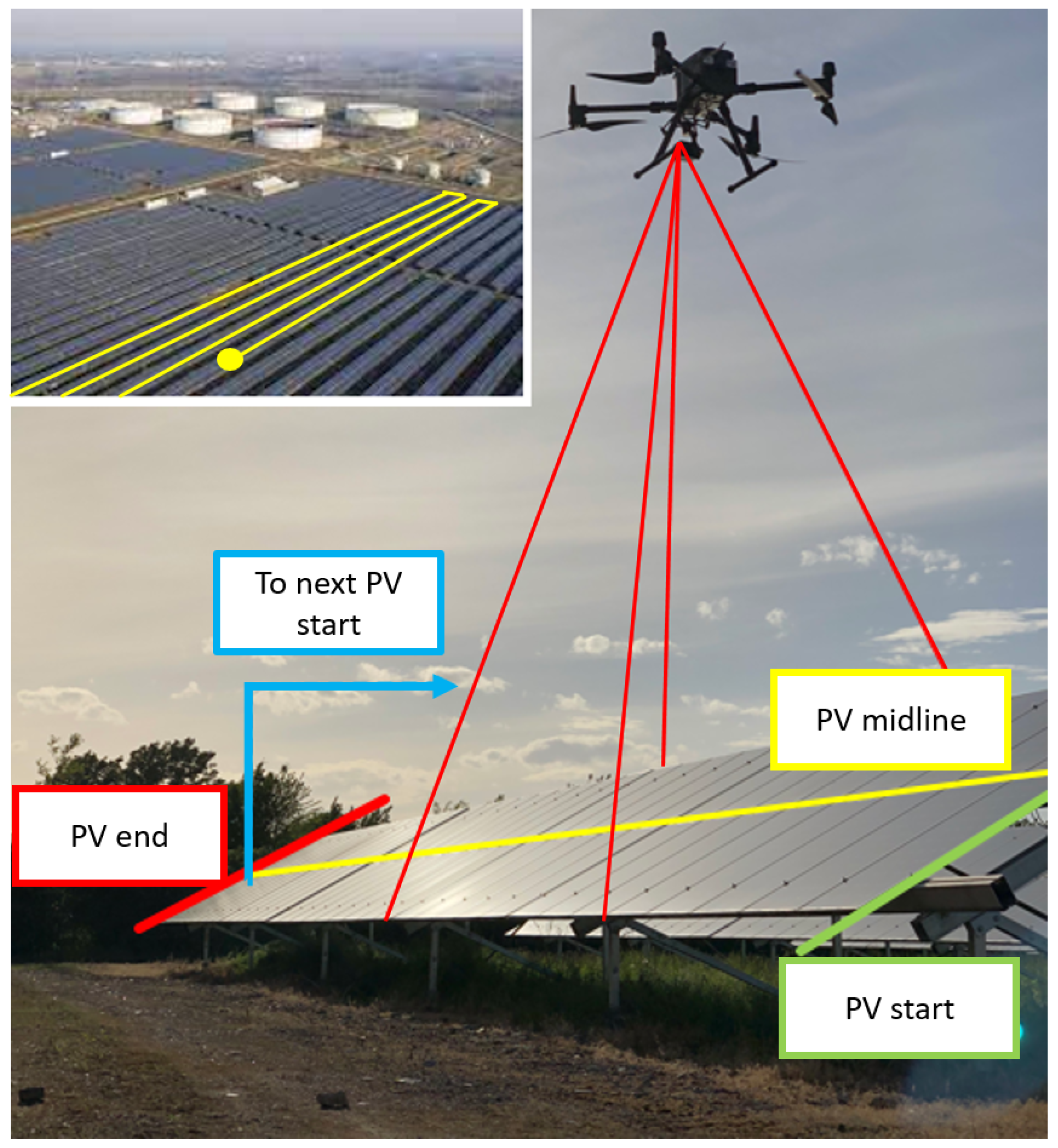
• PV midline, a straight line in the middle of the PV module row that determines the desired motion direction;
• PV end, a point on the PV midline that identifies the end of the PV module row;
• PV start, a point that identifies the start of the new PV module row, whose position is computed with respect to the end of the previous row.

The upper left corner of Figure 1 shows a UAV moving along the PV rows in a boustrophedon way. The UAV moves from PV start to PV end along a PV midline. Then, it “jumps” to the next PV row, and it starts moving again from the following PV start to its corresponding PV end, and so on. Please note that even if panel defect detection is the final goal of UAV-based inspection, this article addresses only UAV navigation and purposely ignores defect detection—which most companies perform offline by analyzing the images acquired along the path through dedicated tools.

The article is organized as follows. Section 2 surveys the relevant literature. Section 3 describes the system architecture. Section 4 introduces the techniques used for PV module segmentation using RGB and thermal images. Section 5 introduces strategies for UAV autonomous navigation. Section 6 and Section 7 present the experimental results in a photorealistic simulated environment and a real PV plant. Finally, in Section 8, conclusions and directives for future research are given.

2. State of the Art

Even if defect detection is not the objective of this article, it is important to highlight previous work in this field as it motivates the application domain we are considering. Researchers proposed various techniques for automatic defect detection from aerial images. For example, the authors of [17,18] use computer vision and machine learning techniques to detect and classify cracks and potholes in roads and highways using images taken by UAVs. Similarly, refs. [19,20] address the inspection of power lines with UAVs, using techniques such as faster region-based convolutional neural network (Faster R-CNN) [21] to detect defects and the Hough transform [22] for cable detection. Strategies for automatic defect detection have also been applied to the PV plant scenario. For example, ref. [23] proposes two different techniques for inspection and mapping, aerial IR/visual image triangulation and terrestrial IR/visual image georeferencing: the authors discuss the potential of both approaches in localizing defective PV modules. In [24], a convolutional neural network (CNN) is used for defect recognition based on aerial images obtained from UAVs. The authors of [25] present an approach that unifies two region-based CNNs (R-CNN) to generate a robust detection approach combining thermography and telemetry data for panel condition monitoring. A model-based approach for the detection of panels is proposed in [26]: this work relies on the structural regularity of the PV module rows and introduces a novel technique for local hot spot detection from thermal images based on a fast and effective algorithm for finding local maxima in the PV panel regions. In [27], a fully automated approach for detecting, classifying, and geopositioning thermal defects in the PV modules is proposed, which exploits a novel method based on image reprojection and function minimization to detect the panels from the images. The work described in [28] proposes a novel method for estimating the power efficiency of a PV plant using data from thermal imaging and weather instruments obtained using a UAV instrumented with a radiometer, a thermometer, and an anemometer. These and similar studies address only the problem of autonomous defect detection and geopositioning without using the acquired images as feedback for the UAV to move autonomously along the inspection path.

The autonomous inspection of PV plants through UAV photogrammetry has been explored in the literature [14,15,29,30]. The UAV is given a set of waypoints, usually arranged in such a way as to cover a delimited area to ensure the required horizontal and vertical overlapping of images. Then, the UAV moves along the planned sequence of waypoints using GNSS/GPS data only, possibly negatively impacting data quality due to positioning errors [31]. An approach to generating an optimal waypoint path based on satellite images is proposed in [32] to reduce the error due to the misalignment of georeferenced images and the actual inspection site. The PV plant’s boundary is extracted via computer vision techniques, and the system can re-compute the path if the UAV requires reaching a specific location (e.g., a PV module where a defect has been detected) or if the UAV cannot complete the initial path for any reason. In [33], a novel technique for boundary extraction is proposed using a Mask R-CNN architecture with a modified VGG16 backbone. The network is trained on the AMIR dataset [34]: an aerial imagery collection of PV plants from different countries. The authors of [35] present a novel way to develop a flight path automatically with coverage path planning (CPP) methods [36] by segmenting the region of interest within PV plant images. The work proposed in [16] uses a VGG16 CNN fed with images that underwent a structure from motion-multiview stereo (SfM-MVS) photogrammetric processing workflow to generate thermal orthomosaics of the inspected sites. These and similar approaches focus on planning a waypoint path with the objective of covering the whole area according to the principles of photogrammetry, i.e., they do not consider tracking individual PV module rows at a lower height from the ground to produce fewer and higher resolution images to be processed.

Visual servoing is widely used in robotics. Many examples of UAV autonomous navigation based on data acquired through cameras exist in the literature, some involving inspection tasks. For example, an algorithm for detecting vertical features from images was used in [11] to guide a UAV along a semi-linear path while flying over a highway in the United States. This approach is based on the consideration that vertical edges are a characterizing attribute of highways that can be easily detected using methods such as RANSAC [37], which can also be used to predict splines [38] where sharp curves may occur. Similar techniques are found in [39,40], where the authors contributed to the fields of precision agriculture and building inspection, respectively. In [39], a novel control technique based on a passivity-based visual servoing controller with dynamics compensation to track crops is described. The proposed system allows a UAV to move along straight lines such as those formed by structured crops. In [40], a complete navigation and inspection task is executed by an autonomous quadrotor. The most interesting part of this work is the approach used for road detection and navigation, which segments the image into predominant color layers before feeding it to DeepLabv3+ [41], a network trained for semantic segmentation. The road is then identified in the image and finally followed by the UAV by defining a sequence of control points. The approach recently proposed in [42] relies on the availability of well-described streets in urban environments for UAV navigation and path tracking: while the drone position is continuously computed using visual odometry, scene matching is used to correct the position drift.

Visual servoing has rarely been applied to UAV navigation over large PV plants. This may be due to the complexity of the scenario, which may have different characteristics in terms of the number of PV module rows, their dimension, and mutual arrangement. Nevertheless, some attempts in this direction have been made in recent years. For example, in [9], the authors propose a vision-based guidance law to track PV module rows based on PV modules’ edge detection. The approach extracts vertical edges from RGB images using a Hough transform. Then, the detected misalignment between the PV row observed from images and the actual UAV position is fed to the navigation control law. Unfortunately, this approach has only been tested in simulation. An edge detection technique was also proposed in [43], where the metallic profile of the PV module rows is detected and segmented by combining color and feature extraction using the Hough transform and a hue–saturation–value (HSV) model. Once the panels have been segmented, the velocity orthogonal to the PV module row is controlled to keep the UAV aligned. Both approaches rely on the tuning of parameters for edge extraction: notwithstanding this limitation, it is worth noting that, in the “era of deep learning”, many of the approaches noted above [9,39,40,43] rely on model-based vision techniques for feature segmentation. In structured environments whose model is a priori known, such as PV plants, a model-based formulation of the problem may offer advantages in predictable and explainable behavior [44] and possibly robustness to adversarial attacks [45] that cannot be ignored. As an aside, this is also confirmed by AI in aviation (particularly machine learning) still in its infancy. Even if AI is widespread in subdomains such as logistics and fuel consumption estimation [46,47], AI techniques in flight control are rarely found in real-world application scenarios.

3. System Architecture

The system can autonomously perform UAV-based PV inspection centered on the following core elements:

• A procedure for detecting PV modules in real time using a thermal or an RGB camera (or both);
• A procedure for correcting errors in the relative position of the PV midline, initially estimated through GPS, by merging thermal and RGB data;
• A navigation system provided with a sequence of georeferenced waypoints defining an inspection path over the PV plant, which uses the estimated position of the PV midline for making the UAV move along the path through visual servoing.

The software architecture implemented in ROS [48] is shown in Figure 2. ROS nodes (1) and (2) acquire and process raw frames from the RGB and the thermal camera and perform PV module segmentation (see Section 4.1 and Section 4.2). As an output of this process, each node returns the parameters, in the image frame, of the straight lines running in the middle of the detected PV module rows. To increase segmentation accuracy with varying environmental conditions, node (3) implements an optimization procedure to find the best parameters for segmentation: some details about this procedure are in Section 4.3. Node (4) merges subsequent observations, independently performed by the two cameras in subsequent time instants. Because the parameters of straight lines independently extracted by (1) and (2) may be affected by errors, an EKF is used to estimate the PV midline by merging the observations provided in real time by nodes (1) and (2) with a priori knowledge (see Section 5.1 and Section 5.2). Finally, node (5) uses the estimated reference path to control the UAV through visual servoing (Section 5).

PV module row tracking is insufficient: node (5) also needs rules to instruct the UAV to move to the next row when the previous one has been completed. This means we need a waypoint-based reference path defining the order according to which PV module rows shall be inspected. Remember that waypoints can be labeled as PV start or PV end and are acquired before the inspection through Google Earth or other georeferenced images (possibly affected by positioning errors) (Figure 1). They are connected in a sequence such that

• the path goes from a PV start to a PV end waypoint when moving along a PV row: in this case, the distance between PV start and PV end defines how far a PV midline shall be followed before moving to the next one;
• the path goes from a PV end to a PV start waypoint when jumping to the next PV row: in this case, the position of PV start relative to PV end defines the start of the new row with respect to the previous one.

Currently, waypoints are manually chosen, but this process might be automated starting from a georeferenced image of the whole plant.

As already discussed, real-time segmentation and visual tracking of PV module rows may play a key role in successful navigation. Indeed, waypoint-based navigation relying on the embedded positioning system of the UAV (typically merging GPS, IMUs, and compass) has well-known limitations: the absolute position of PV start and PV end waypoints, as well as GPS data, may be affected by large errors in the world frame. In contrast, by using visual servoing to move along a PV row, we only need to ensure that the relative position of adjacent waypoints and the small UAV displacement from a PV module row to the next one performed with GPS only are sufficiently accurate. Figure 3 shows this concept: the colored part of the figure represents a priori computed waypoints; the gray part represents the observed position of PV module rows while tracking them. The proposed solution works even when the absolute error between the a priori computed and the observed position of PV module rows is huge, given that $\Delta l\approx \Delta l^{\prime }$ and $\Delta p\approx \Delta p^{\prime }$ (the additional requirement $l\approx l^{\prime }$ holds if one uses GPS to measure the length of the PV module row instead of implementing some sort of “end-of-row detector”). These assumptions look reasonable, as georeferenced waypoints computed from Google Earth images and GPS data may be affected by large biases (which, in the case of GPS, vary with time) but tend to be locally coherent—i.e., the relative error of waypoints (respectively, GPS data) with respect to previous waypoints (respectively, GPS data acquired in nearby locations) is small.

Eventually, even if it is not the focus of this article, note that additional high-resolution thermal images (not used for navigation) are captured and stored in the onboard storage of the UAV for defect detection (possibly performed after the UAV has ended the mission). In this case, the UAV’s flying height and speed determine the acquisition frequency to guarantee that images overlap.

4. Detection of PV Modules

4.1. Segmentation of PV Modules via Thermal Camera

Each image captured by the thermal camera can be represented as a matrix. The image frame I is in the upper-left corner of the image plane, and $i(u,v)$ is a function that associates a thermal value to each pixel $(u,v)$: thermal cameras return the thermographic image as a mono-channel grayscale intensity matrix, where the intensities of the pixels may assume values between 0 and 255.

As a first step, a mask F is applied to the image after choosing two thresholds $t{h}_1$ and $t{h}_2$. That is, each image pixel is processed as follows:

$$f(u,v)=\left\{\begin{array}{cc}i(u,v),\hfill & \mathrm{if} t{h}_1<i(u,v)<t{h}_2\hfill \\ 0,\hfill & \mathrm{otherwise}.\hfill \end{array}\right.$$

(1)

Although the values of $t{h}_1$ and $t{h}_2$ may be a priori chosen based on the analysis of previously acquired images (in our case, a dataset of images of a PV plant through a DJI Zenmuse H20T camera, composed of 430 $640\times 512$ thermal images) by manually inspecting the range of thermal values that will likely allow for the segmenting of panels from the ground under different daylight conditions, there may be the need to fine-tune them when environmental conditions change. Please refer to Section 4.3 concerning the strategy used for this purpose. As expected, and visible in Figure 4a, this mask is not sufficient to make the PV modules emerge unambiguously: in some regions, the ground may have the same temperature as the panels.

As a second step, we filter out the noise by exploiting a priori domain knowledge: even if pixels with thermal intensity in the selected range can also be found outside PV panels, the panels are characterized by a higher density of pixels falling within the thresholds. Then, the entire image is filtered by computing a distance matrix D, storing the Euclidean distance of each pixel in F from the closest pixel whose value is zero. That is, for each pixel $(u,v)$, we compute:

$$d(u,v)=\sqrt{{(u_{zero}-u)}^2+{(v_{zero}-v)}^2}$$

(2)

where $u_{zero}$ and $v_{zero}$ are, respectively, the row and the column of the zero value pixel nearest to $(u,v)$; see Figure 4b.

As a third step, each pixel of the distance matrix D is transformed into a binary intensity value as follows:

$$b(u,v)=\left\{\begin{array}{cc}1,\hfill & \mathrm{if} d(u,v)>t{h}_3\hfill \\ 0,\hfill & \mathrm{otherwise}\hfill \end{array}\right.$$

(3)

where $t{h}_3$ can be interpreted as a distance threshold to determine whether a pixel $(u,v)$ in the original image belongs to a high-density region; see Figure 4c. As for $t{h}_1$ and $t{h}_2$, the threshold $t{h}_3$ is set a priori and then fine-tuned with the optimization procedure described in Section 4.3. Groups of neighboring pixels are clustered into N polygonal regions $S_i$: during the process, only the regions larger than a given number of pixels survive, whereas smaller clusters are deleted (OpenCv function findcontours.). The distance matrix D is quite a powerful tool for estimating the position of the PV modules in the image. Nevertheless, the figure shows that it can fail, especially when the surface of the panels is not equally heated, presenting regions with different temperatures. The next step addresses this problem.

As a fourth step, we compute, for each segmented region $S_i$, a regression line through polynomial curve fitting (OpenCv function fitLine.): starting from regions $S_i$, N regression lines are computed, each described by a point $p_i=(u_i,v_i)$ and a unitary vector $l_i$ defining a direction in the image plane I; see Figure 4d.

As a fifth step, the detection algorithm requires clustering all regions $S_i$ that are likely to correspond to PV modules aligned in the same row by using their corresponding regression lines. That is, starting from a subset of individual shapes $S_i$ and the corresponding regression lines, a unique cluster $C_j$ (more robust to noise) is computed. Specifically, two regions $S_i$ and $S_k$ are clustered in $C_j$ if

• the corresponding regression lines tend to be parallel;
• the average point–line distance between all pixels in the image plane belonging to the first line and the second line is below a threshold, i.e., the two lines tend to be close to each other.

The clustering technique is iteratively applied for all the shapes $S_i$: then, a new regression line is computed for each cluster $C_j$; see Figure 4e. The final output of the process is a set of J lines, each possibly corresponding to multiple PV modules belonging to the same row. Each observed PV midline is represented in the image frame through a couple of points $p_j^{\prime }=(u_j^{\prime },v_j^{\prime })$ and $p_j^{″}=(u_j^{″},v_j^{″})$ corresponding to the intersection of the line with the borders of the image.

4.2. Segmentation of PV Modules via RGB Camera

The algorithm developed to process thermal images is almost completely reused for RGB images, except for the initial steps required for PV module segmentations; see Figure 5a,b.

When using RGB images, the rows of PV modules can be detected due to their color in contrast with the background. Then, as a first step, the original image I is transformed into the hue–saturation–value (HSV) color space: Figure 5a shows the result, RGB-rendered by using H values for the R channel, S for G, and V for B. As a second step, the PV modules are segmented from the background by thresholding the image in all the three HSV channels; see Figure 5b. The lower HSV thresholds $t{h}_4$, $t{h}_5$, $t{h}_6$ and the higher HSV thresholds $t{h}_7$, $t{h}_8$, $t{h}_9$ are manually chosen based on a priori domain knowledge and then fine-tuned before operations, as explained in Section 4.3.

The result is a binary image defined as follows:

$$b(u,v)=\left\{\begin{array}{cc}1,\hfill & \mathrm{if} t{h}_4<H(u,v)<t{h}_7\hfill \\ \hfill & \wedge t{h}_5<S(u,v)<t{h}_8\hfill \\ \hfill & \wedge t{h}_6<V(u,v)<t{h}_9\hfill \\ 0,\hfill & \mathrm{otherwise}\hfill \end{array}\right.$$

(4)

Please remember that, in the HSV color space, hue is measured in degrees from 0 to 360 and is periodic (In OpenCV, hue is encoded in a byte and ranges from 0 to 179): red takes negative and positive values around zero, which means that the first condition in (4) must be changed to “$\mathrm{if} \mathrm{not} (t{h}_4\le H(u,v)\le t{h}_7)$” in case we need to segment areas characterized by a reddish color.

The final steps of the process, as for thermal images, require segmenting polynomial regions $S_i,\dots ,S_N$ in $b(u,v)$, each associated with a regression line, which are finally clustered into J clusters $C_j$, each corresponding to an observed line $o_j=(p_j^{\prime },p_j^{″})$; see Figure 5c,d.

4.3. Threshold Tuning

PV module detection needs appropriate thresholding. For thermal images, we must choose the lower and upper bounds $t{h}_1$ and $t{h}_2$ of thermal intensity in (1) and the distance threshold $t{h}_3$ in (3); for RGB images, we need to choose the minimum $t{h}_4$, $t{h}_5$, $t{h}_6$ and the maximum $t{h}_7$, $t{h}_8$, $t{h}_9$ values for each HSV channel in (4). Thresholds are chosen using a procedure that maximizes the number of PV modules detected in thermal and RGB images separately taken as well as the matches between the PV modules detected in both images. The following assumes that thermal and RGB images overlap, which can be ensured through rototranslation and scaling if needed. Under this constraint, despite the segmented PV module shapes being slightly different depending on the acquisition method used (in thermal images, the temperature of the junctions between adjacent PV panels is usually different from the PV panels themselves, resulting in a sequence of smaller rectangular shapes; in RGB images, this never happens: segmentation returns larger rectangular areas composed of multiple panels), they are expected to roughly correspond to rectangular shapes, whose dimensions can be predicted depending on the geometry of PV panels and the UAV’s flying height, which occupy the same regions in pairwise images.

The algorithm used to minimize the cost function is L-BFGS-B [49], a limited-memory algorithm that can be used to minimize a non-linear cost function subject to simple bounds on the variables. The algorithm is particularly appropriate for solving large non-linear, non-convex optimization problems in which the Hessian is difficult to compute.

We assume that the UAV reaches the start position of the first PV module, possibly remotely controlled by a human operator, with its front oriented towards the direction of the PV module row. Then, the following non-linear, non-convex optimization problem on variables $t{h}_i$, $i=1\dots 9$, is solved:

$$\underset{t{h}_1-t{h}_9}{min}-\sum _{i=1}^{N^T}(c_i^T+r_i^{TR})-\sum _{i=1}^{N^R}(c_i^R+r_i^{RT})$$

(5)

where (5) is the cost function, whose value expresses the “quality” of the segmentation algorithm given a set of thresholds $t{h}_1-t{h}_9$ subject to disequality constraints.

Mathematical details of the cost are not discussed for the sake of brevity. Intuitively, please remember that the thermal camera computes a set of $N^T$ segmented regions $S_i$, $i=1\dots N^T$, and the RGB camera computes a set of $N^R$ segmented regions $S_i$, $i=1\dots N^R$. Then, the first sum in the cost function refers to regions extracted from the thermal camera, and the second sum refers to regions extracted from the RGB camera. For each region $S_i$ extracted from thermal images, the cost function comprises two terms $c_i^T$ and $r_i^{TR}$. The term $c_i^T$ intuitively considers how close $S_i$ is to a rectangular shape oriented along the current direction of motion and how close $S_i$’s extension is to a value that depends on the PV module geometry and the UAV height from the ground. The term $r_i^{TR}$ measures the pixel-wise correlation between the region $S_i$ and the binary mask extracted from the paired RGB image covering the same area: $r_i^{TR}$ is higher if the region $S_i$ segmented from the thermal image is also present in the RGB image. The two terms $c_i^R$ and $r_i^{RT}$ are computed similarly, starting from regions extracted from RGB images.

Please note that jointly optimizing all variables might be time-consuming: for this reason, during experiments in PV plants, we decompose problem (5) into two sub-problems. First, we only consider RGB images and search for the minimum of $-{\sum }_{i=1}^{N^R}{c}_i^R$: that is, we ignore correlation with thermal images. Second, we consider thermal images only and search for the minimum of $-{\sum }_{i=1}^{N_T}(c_i^T+r_i^{TR})$. This simplification seems a good compromise to reduce computation time if we want to repeat the procedure, e.g., at the PV start of each new row.

5. UAV Navigation

5.1. From the Image Frame I to the Camera Frame C

To describe the motion of the UAV body in the world frame, we define a mobile camera frame C with origin in the center of the camera lens, $xy$−plane parallel to the $uv$-image plane at a distance f (focal length), x-axis pointing to the UAV front, and z-axis downward (that is, x heads towards $-v$ in the image plane, and y heads towards u; see Figure 6). The origin of the camera frame moves as the UAV moves along the PV module row: because the UAV is endowed with a gimbal mechanism that keeps the $xy$−plane of the camera frame parallel to the $xy$−plane of the world frame W, all the transformations involving the image, world, or camera frame (respectively, I, C, W) are simpler, as the camera is always looking perpendicularly to the ground in a nadiral position.

Given a point $p_i=(u_i,v_i)$ expressed in pixel coordinates in the image frame I, by supposing that the point corresponds to a feature on the ground, its position $(x_i^C,y_i^C,z_i^C)$ in the camera frame C can be computed as:

$$x_i^C=-\frac{k}{f}(v_i-\frac{V}{2})z_g$$

(6)

$$y_i^C=\frac{k}{f}(u_i-\frac{U}{2})z_g$$

(7)

$$z_i^C=z_g$$

(8)

where U and V denote, respectively, the axes of the image frame, k converts the pixel size in meters, $z_g>0$ is the distance of the ground from the origin of the camera frame, and $f<0$ is the focal length. The thermal and RGB cameras are typically mounted on the same rigid body a few centimeters apart in commercial products. Then, if we set C’s origin in the thermal camera lens, all observations done in the RGB image frame should ideally undergo a transformation to map them in C. This is not noted in the following for brevity’s sake. Using the formula above, for every observed line described by $p_i^{\prime }=(u_i^{\prime },v_i^{\prime })$ and $p^{″}=(u_i^{″},v_i^{″})$ in the image frame I returned by the procedure in Section 4 (either by the thermal or RGB camera), we compute the corresponding points in the camera frame C and then the parameters $o_i^C=(a_i^C,b_i^C)$ of an observed line $y^C-a_i^C{x}^C-b_i^C=0$ in C through simple geometrical considerations. Please note that we can ignore the $z^C$ coordinate here because the $xy$ plane of the camera frame is parallel to the ground due to gimbal stabilization: the UAV altitude will be separately controlled through an independent mechanism. Then, the equation $y^C-a_i^C{x}^C-b_i^C=0$ should be better interpreted as the equation of a plane perpendicular to the $xy$ plane of the camera frame C.

5.2. Path Estimation through EKF

The sequence of observations $o_k^C=(a_k^C,b_k^C)$ acquired in subsequent time steps k, either extracted from the same image or subsequent images, are iteratively merged to estimate the actual PV midline in the world frame. Specifically, we represent the actual PV midline through parameters $m^W=(a^W,b^W)$, which describe a straight line in W with implicit equation $y^W-a^W{x}^W-b^W=0$ (once again, this should be better interpreted as a plane perpendicular to the ground). For this purpose, an extended Kalman filter [50] is used. Please note that the state $m^W=(a^W,b^W)$ of the PV midline is described in the world frame W to keep the system dynamics constant: due to this choice, the state $m^W$ to be estimated does not change with respect to W as the UAV moves along the PV module row. However, the observations $o_k^C=(a_k^C,b_k^C)$ acquired through cameras at steps k are expressed in the camera frame C; to correct the state’s estimate $m^W$ through observations $o^C$, the system will need to map observations onto the world frame W through the EKF observation matrix H, which, in turn, requires knowing the UAV pose.

In this work, we assume that the pose $x^W,y^W$, and yaw ${\theta }^W$ of the camera frame in the world frame is computed by the low-level flight controller embedded in the UAV, which typically merges GPS, IMUs, and compass. Once again, due to the gimbal mechanism and the fact that we control the altitude through an independent mechanism, $z^W$ is ignored because the pitch and roll of the camera can be approximated to be zero. Using the embedded UAV positioning system may be counter-intuitive, as we repeatedly stated that it is affected by absolute errors. However, similar to what happens in the passage from one PV module row to the next one (Figure 3), it is deemed appropriate as we are not interested in knowing the absolute UAV pose with high accuracy. It is sufficient that the pose error slowly changes in time and that it is almost constant along one PV module row (which typically happens with GPS low-frequency errors) to guarantee that subsequent observations are coherent with each other when mapped to the world frame without producing abrupt changes in the state estimate. (Ideally, we could attempt to estimate the UAV pose in the world frame by merging the sensors above with the observations made with cameras, by hypothesizing an augmented state vector including both the PV midline and the UAV pose [51]. However, this possibility is not explored in this work.)

The EKF allows for merging observations acquired at different times from the thermal and RGB cameras. In the following, we use the notation ${\hat{m}}_{k+1|k}^W={\hat{m}}_{k|k}^W$ to describe the evolution of the state at the prediction step $k+1$ due to control inputs (which, as already noted, is constant), and the notation $o_{k+1}^C=(a_{k+1}^C,b_{k+1}^C)$ to describe the observation made at the update step $k+1$ by the thermal or RGB sensor.

During the update step, we need a measurement model ${\widehat{o}}_{k+1}^C=H_{k+1}{\hat{m}}_{k+1|k}^W$, where $H_{k+1}$ is the Jacobian of the non-linear observability function $h(m)$, which allows for obtaining the expected measurement ${\widehat{o}}_{k+1}^C$ from the estimated state ${\hat{m}}_{k+1|k}^W$ given the current camera position and yaw $x^W,y^W,{\theta }^W$. Specifically, $h(m^W)$ has two components:

$$\begin{array}{c}\hfill h_1(m^W)=\frac{a^W-tan{\theta }^W}{1+a^{W}tan{\theta }^W}\\ \hfill h_2(m^W)=\frac{x^W{a}^W+b^W-y^W}{cos\theta +sin\theta a^W}\end{array}$$

(9)

whose Jacobian with respect to $(a^W,b^W)$ needs to be evaluated in ${\hat{a}}^W,{\widehat{b}}^W,x^W,y^W$, and ${\theta }^W$. The EKF is a recursive algorithm consisting of two steps: state prediction and update. The prediction at step $k+1$ can be expressed as:

$${\hat{m}}_{k+1|k}^W=A{\hat{m}}_{k|k}^W+B{u}_{k|k},$$

(10)

where A, in our case, is the identity matrix, and $B=0$ because the state $m^W$ is invariant over time when expressed in world coordinates. The state equations are linear, and the EKF is needed only because of the non-linearity of the observation model. The error covariance matrix is

$$P_{k+1|k}=A{P}_{k+1|k}{A}^T+Q,$$

(11)

where the process noise $Q\approx 0$. As the state is not evolving, Q should be null: nevertheless, we empirically add a very small contribution to the error covariance matrix to ensure that new observations will continue to contribute to the state estimate.

Only the actual observations $o_{k+1}^C$ that are “sufficiently close” to the expected observations ${\widehat{o}}_{k+1}^C$ (in the same spirit adopted for clustering in Section 4) are considered during the update step. In contrast, outliers are rejected to avoid undesired corrections due to the detection of neighboring PV rows running in parallel to the tracked one. Finally, in the correction step, the Kalman gain is computed starting from the covariance of the measurement noise R and P as usual:

$$K_{k+1}=P_{k+1|k}{H}_{k+1}^T{(H_{k+1}{P}_{k+1|k}{H}_{k+1}^T+R)}^{-1}.$$

(12)

The a posteriori estimate is updated as:

$${\hat{m}}_{k+1|k+1}^W={\hat{m}}_{k+1|k}^W+K_{k+1}(o_{k+1}^C-{\widehat{o}}_{k+1}^C),$$

(13)

$$P_{k+1|k+1}=(I-K_{k+1}{H}_{k+1})P_{k+1|k}.$$

(14)

The covariance matrix R relative to the thermal or RGB cameras is evaluated experimentally and takes into account both segmentation errors due to the procedure in Section 4 and the fact that, during an inspection, the GPS error may be subject to minor variations, therefore partially conflicting with the assumption of a constant GPS error in (9).

The EKF is initialized with ${\hat{m}}_{0|0}^W=(a^W,b^W)$ estimated at step $k=0$ by considering the two waypoints PV start and PV end of the initial PV module row.

5.3. Path Following

Path following works in two different phases: (i) when the UAV is moving from PV start to PV end along a PV module row; (ii) when it is moving from PV end of the current row to PV start of the next one (Figure 3).

In phase (i), navigation is based on PV midline tracking through visual servoing. After each iteration of the EKF, the estimated parameters describing the PV midline in the world frame are mapped back onto the camera frame for path-following, yielding $(a_{ref}^C,b_{ref}^C)$. Then, given the equation $y^C-a_{ref}^C{x}^C+b_{ref}^C=0$ in the camera frame, the distance error

$$e=-b_{ref}^C/{(a_{ref}^{C2}+1)}^{1/2}$$

(15)

is computed, as well as the parallel and the perpendicular vectors to the path

$$\begin{array}{cc}\hfill V_{\Vert }^C=(1/a_{ref}^C,1),& V_{\perp }^C=(-1,1/a_{ref}^C).\end{array}$$

(16)

Once the quantities above have been computed, different approaches can be used to control the distance from the PV midline. In this work, we adopt a simple “carrot chasing” approach [52]: the parallel and perpendicular vectors are added to compute the position of a virtual moving target using the distance error e as a weighting factor for $V_{\perp }^C$, and a PID controller is used to tune the UAV velocities to regulate the distance from the target to zero.

In phase (ii), the UAV uses the pose information $x^W$, $y^W$, ${\theta }^W$ returned by the onboard flight controller (merging GPS, IMU, and compass) to move from PV end to the next PV start. In both phases, the altitude is separately controlled using embedded sensors returning the height from the ground (a method to automatically control the UAV altitude depending on the difference between the actual and expected dimensions of PV modules on the image plane was implemented, but it is not discussed in this work).

6. Material and Methods

This and the following sections present the experiments conducted in a real PV plant and a realistic simulation environment.

Real-world experiments in a PV plant were conducted using a DJI Matrice 300 aircraft equipped with a DJI Zenmuse XT2 camera; see Figure 7. The camera has a field of view of $57.12\times 42.44$ degrees and a gimbal mechanism. An onboard DJI Manifold PC equipped with an NVIDIA Jetson TX2 and 128GB of internal memory performs all the computations described in previous sections to process the acquired images and control the UAV.

The simulation environment deserves more attention (Figure 7). In addition to the onboard DJI Manifold performing the core computations, two programs were running in parallel to simulate, respectively, the dynamics and the perception of the UAV:

• The DJI Matrice Simulator embedded in the DJI Matrice 300. When the DJI Manifold is connected to the drone and the OSDK is enabled, this program simulates the UAV dynamics based on the commands received from the ROS nodes executed on the DJI Manifold.
• The Gazebo Simulator, running on an external Dell XPS notebook with an Intel i7 processor and 16 GB of RAM, integrated with ROS. Here, only the thermal and RGB cameras and the related gimbal mechanism are simulated to provide the DJI Manifold with images acquired in the simulated PV plant.

The cameras’ position inside Gazebo is linked to the UAV position returned by the DJI Matrice Simulator to guarantee coherence in the simulated images returned during the simulated flight.

Specifically, RGB textures are placed “above in the sky”, whereas thermal textures are placed “below on the ground”. By adding two cameras in Gazebo, one directed towards the sky and the other directed towards the ground, we can simulate the acquisition of RGB and thermal images of the same PV plant. Textures were produced from images captured by the DJI Zenmuse XT2 during a PV plant inspection in northern Italy.

Both in real-world experiments and in simulation, we initially compute the “reference waypoint path” to be followed by the UAV by considering PV module rows one after the other in boustrophedon mode. Once the UAV has reached the PV start of the first PV row, we execute the optimization process for tuning thresholds depending on environmental conditions by letting the UAV hover at a certain height over the PV module. Then, the UAV starts moving using both cameras and the EKF for iteratively extracting the PV midline, correcting the reference path, and moving along it. When the UAV reaches PV end, the visual tracking stops, and the UAV moves to the next PV start. We consider the mission completed when the UAV has inspected the required number of parallel PV module rows.

The thermal and RGB images are processed, at an approximate frequency of 3 and 5 fps, respectively, both in the simulated and real experiments (computations can likely be made more efficient to achieve a higher frame rate). Observations are used to correct the estimate of the PV midline through the EKF. Then, velocity commands for path-following are computed and sent to the onboard controller of the DJI Matrice 300 approximately with a 5 Hz frequency in simulation (due to heavy computations performed in Gazebo) and a 30 Hz frequency in real cases. Simulated experiments (Section 7.2) were mainly aimed at validating the proposed approach and assessing the system’s reliability in the presence of inaccurate waypoint positioning. Experiments in the real scenario (Section 7.3) had the primary purpose of comparing the proposed approach’s robustness and assessing advantages deriving from combining thermal and RGB cameras.

7. Results

7.1. Threshold Optimization Time

We analyzed the time required to perform the optimization procedure described in Section 4.3 on RGB and thermal images collected during different flights with different daylight conditions.

Table 1. Threshold selection times in different tests.

Test #	${\mathit{t}}_{\mathit{HSV}}$ [s]	${\mathit{t}}_{\mathit{thermal}}$ [s]	${\mathit{t}}_{\mathit{tot}}$ [s]	Month	Time of Day
1	78.2	34.7	112.9	Jun	9:25 am
2	85.1	55.2	140.3	Oct	10:26 am
3	72.3	49.0	121.3	Jul	12:09 pm
4	68.6	38.9	107.6	Oct	1:20 pm
5	82.3	44.5	126.8	Mar	3:19 pm

shows, for five subsequent tests in different environmental conditions from early morning to mid-afternoon, the time $t_{HSV}$ required for HSV optimization (thresholds $t{h}_4-t{h}_9$), the time $t_{thermal}$ required for thermal optimization (thresholds $t{h}_1-t{h}_3$), and the overall time $t_{tot}$ required by the L-BFGS-B algorithm to complete the process.

As visible from the results, the optimization algorithm is reasonably fast in finding a suitable range of threshold values to detect and cluster PV module rows in the images, even in the presence of possible misalignments between the two images. Tests show that the optimization time can vary depending on the number of PV module rows in each image and daylight conditions, but only minimally. However, please observe that appropriate light conditions also play a crucial role in defect detection (not addressed in this article). Flying during cloudy days or at night does not deserve to be explored because the detection of defects in the PV modules can be unreliable due to the low temperature reached by the panel surface. Consider that the time range between 9 am and 7 pm is known to be appropriate for thermal image acquisition only in summer. In contrast, this time range is much shorter at other times of the year, which is compatible with the results achieved in all navigation tests.

Finally, the experiments described in the following sessions were performed with images collected at different times and on different days. In all experiments, we noticed that the choice of the thresholds $t{h}_1-t{h}_9$, once performed, tends to work well for the whole experiment duration, making it possible to execute the optimization algorithm only at the beginning of each flight.

7.2. Results in Simulation

Two classes of experiments were performed in the simulation:

• Section 7.2.1 reports the simulated experiments with the thermal camera only, RGB camera only, and both cameras for PV module detection. Here, we do not consider errors in waypoints, which are correctly located on the midlines of the corresponding PV rows.
• Section 7.2.2 reports the simulated experiments with both cameras to assess the robustness of the approach in the presence of errors in waypoint positioning.

7.2.1. Navigation with Thermal Camera Only, RGB Camera Only, and Both Cameras

The mission consisted of inspecting four parallel PV rows. The waypoints were assumed to be correctly placed at each row’s start and end without errors. During navigation, the UAV velocity had a constant value of $0.6$ m/s, and the UAV flew at a constant height of 15 m from the take-off point. Please note that, at a 15 m height, a speed lower than 2 m/s is appropriate to prevent blurred images and ensure image overlapping.

Experiments were initially performed with the thermal camera only. In Figure 8, the projection on the xy−plane of the path followed by the UAV along four parallel PV rows (blue line) and the reference path determined by the waypoints (red dashed line) are shown. After take-off, the UAV autonomously reached the first PV start, and hovered there for some seconds before moving along the panels, collecting observations to estimate the PV midline. Navigation performance can be evaluated by measuring the convergence of the UAV position to the midline of PV module rows.

In Figure 9, the error between the real PV midline described by $m=(a^W,b^W)$ (the ground truth is known in simulation) and the estimated state $\hat{m}=({\hat{a}}^W,{\widehat{b}}^W)$ returned by the EKF is shown. Green vertical lines correspond to PV start; red vertical lines correspond to PV end of the same row. Because the UAV moved from the end of one row to the start of the next one by using positioning information provided by the onboard flight controller, the plots included between a red vertical line and the subsequent green line are ignored, as they correspond to a change of PV module row.

In Figure 10, the control error e between the UAV position and the PV midline estimated with the EKF is shown, with average ${\mu }_e=0.022$ m and standard deviation ${\sigma }_e=0.031$ m (we consider only values included between a green vertical line and the subsequent red vertical line).

In Figure 11, the navigation error $\xi$ between the UAV position and the actual PV midline (the ground truth is known in simulation) is shown. The evaluated RMSE${}_{\xi }$ (root mean squared error) during navigation, computed from $\xi$, is $0.178$ m. The figure shows that the navigation error tends to be larger when the UAV starts to track the PV module row after reaching PV start, the green vertical line. This is coherent with the fact that PV start is considered to be reached when the UAV position is within a 1 m distance, thus producing an initial error that is recovered later.

Next, experiments were performed with the RGB camera only. The projection on the xy−plane of the UAV path using the RGB camera is not reported, as it is difficult to appreciate differences from the previous experiment. Figure 12 reports the error between the actual and the estimated state of the PV midline. Figure 13 reports the control error, with average ${\mu }_e=0.032$ m and standard deviation ${\sigma }_e=0.036$ m (i.e., performance is worse than those obtained during the experiment with the thermal camera). Figure 14 reports the navigation error, with an RMSE${}_{\xi }$ of $0.246$ m.

Eventually, experiments were performed with both cameras. Figure 15 reports the error between the actual and the estimated state of the PV midline. Figure 16 reports the control error, with average ${\mu }_e=0.026$ m and standard deviation ${\sigma }_e=0.036$ m. Figure 17 reports the navigation error with an RMSE${}_{\xi }$ of $0.153$ m.

By considering the estimated parameters ${\hat{a}}^W$ and ${\widehat{b}}^W$ of the PV midline with thermal, RGB, and both cameras (Figure 9, Figure 12 and Figure 15), we can compute the root mean squared error RMSE${}_a$ and RMSE${}_b$ performed in estimating the actual parameters $a^W$ and $b^W$.

Table 2. Control, navigation, and PV midline estimation errors with thermal, RGB, and both cameras.

Test #	${\mathit{\mu }}_{\mathit{e}}$ [m]	${\mathit{\sigma }}_{\mathit{e}}$ [m]	RMSE${}_{\mathit{\xi }}$ [m]	RMSE${}_{\mathit{a}}$	RMSE${}_{\mathit{b}}$ [m]
Thermal camera	0.022	0.031	0.178	0.015	0.173
RGB camera	0.032	0.036	0.246	0.018	0.218
Both cameras	0.026	0.036	0.153	0.016	0.122

reports a summary of the control, navigation, and PV midline estimation errors with thermal, RGB, and both cameras. The RMSE${}_{\xi }$ values in the table show that using both cameras has a slightly positive impact on navigation errors. Similarly, the RMSE${}_a$ and RMSE${}_b$ values show that using both cameras positively impacts the estimated straight-line intercept ${\widehat{b}}^W$ and has a negligible negative impact on the estimated slope ${\hat{a}}^W$.

7.2.2. Navigation with Errors in Waypoint Positions

Tests were performed by considering large errors in the positions of waypoints at the start and at the end of PV module rows to simulate inaccurate waypoint positions computed from Google Earth images. An example is shown in Figure 18, with navigation performed using both cameras: waypoints do not correspond to PV start and PV end of actual PV module rows, as they are subject to a rototranslation error plus additional noise.

However, observing the actual UAV’s path (blue curve in Figure 18) shows that the UAV reached the correct PV start on the second, third, and fourth PV row, thus compensating for large errors due to wrong waypoint placement. Figure 19 reports errors in the PV midline state estimated by the EKF. The control and navigation errors are comparable with those of the previous experiments: the control error in Figure 20 has an average ${\mu }_e=0.022$ m and standard deviation ${\sigma }_e=0.033$ m. The RMSE${}_{\xi }$ computed from the navigation error in Figure 21 is $0.150$ m, comparable with previous experiments.

7.3. Results in Real-World Experiments

Experiments were conducted in a PV plant in Predosa in Northern Italy, exploring different configurations:

• Section 7.3.1 explores navigation along one PV module row using the thermal camera only, RGB camera only, and both cameras.
• Section 7.3.2 explore navigation along four PV rows using both thermal and RGB cameras.

The UAV moved at the desired height from the ground of 15 m and the desired speed of 1 m/s (first three tests) and $1.2$ m/s (fourth test). Please note that the speed is higher with respect to the simulated experiments presented in the previous sections, due to the different control frequencies: 30 Hz in the real experiments versus 5 Hz in the simulation. For the same reason, comparing the system’s performance in simulated versus real-world experiments is inappropriate.

7.3.1. Navigation along One Row

An example of PV module detection in Predosa obtained using the thermal camera is shown in Figure 22 on the left (image taken in the month of November at 2:55 pm, Italian local time).

In Figure 23, the projection on the xy−plane of the UAV path is shown. After take-off, the UAV was manually guided to the first waypoint: in this phase, the control error e and the navigation error $\xi$ are not computed, which explains why they are constantly zero in Figure 24, Figure 25, Figure 26, Figure 27, Figure 28, Figure 29, Figure 30, Figure 31 and Figure 32. Next, the UAV started collecting observations to estimate the parameters ${\hat{a}}^W$ and ${\widehat{b}}^W$ of the PV midline. Because the UAV does not move until the estimation error is below a given threshold at the PV start of each row, the duration of this phase may vary in different experiments or when tracking different PV rows within the same experiment. The average control error and the RMSE${}_{\xi }$ associated with the navigation trajectory are computed only after the UAV has reached the speed of 1 m/s after a transit (i.e., the sometimes significant errors at the start of PV rows are not considered).

Please also note that, in real-world experiments, the UAV path and the position of the PV module row in the world, Figure 23 and Figure 30, were estimated using a GPS. However, we did not use this information for path-following but for visualization purposes only. In all experiments, PV tracking was performed during navigation using the control method described in the previous sections. The navigation error $\xi$ was computed by manually inspecting the video stream acquired by onboard cameras (once again because the ground truth is unavailable in this case). To this end, the video stream was periodically sampled (with a period of approximately four seconds), and images were manually inspected to measure the distance in pixels and then in meters (the meters/pixel ratio is computed by knowing the width in meters of a PV module and measuring its corresponding width in pixels in the image) between the center of the image and the center of the PV module row ($\xi$ tends to zero as this distance tends to zero).

In Figure 24, the control error e is shown (i.e., the distance from the estimated PV midline), with a significant initial error due to inaccurate detection of the PV midline (which was later recovered), average ${\mu }_e=0.012$ m, and standard deviation ${\sigma }_e=0.010$ m. In Figure 25, the navigation error $\xi$, computed as described before, is shown (i.e., the distance from the actual PV midline), with RMSE${}_{\xi }$ of $0.157$ m.

An example of PV module detection using the RGB camera only is shown in Figure 22 on the right (image taken in the month of November at 12:50 pm Italian local time). The projection on the xy−plane of the UAV path is not reported, as it would be difficult to appreciate differences with the previous test. In Figure 26, the control error e is shown, with average ${\mu }_e=0.023$ m and standard deviation ${\sigma }_e=0.019$ m. In Figure 27, the navigation error $\xi$ is shown. The RMSE${}_{\xi }$ is $0.128$ m.

The same test was performed with both the thermal and RGB cameras for PV midline estimation and navigation. Once again, the UAV path is not reported, as it would be challenging to appreciate differences from the previous tests. In Figure 28, the control error e is shown, with ${\mu }_e=0.010$ m and ${\sigma }_e=0.008$ m. In Figure 29, navigation error $\xi$ is shown, with an RMSE${}_{\xi }$ of $0.055$ m. The average navigation error is lower than in the previous cases, as is also visible in the figure.

Table 3. Control and navigation errors with thermal, RGB, and both cameras.

Test #	${\mathit{\mu }}_{\mathit{e}}$ [m]	${\mathit{\sigma }}_{\mathit{e}}$ [m]	RMSE${}_{\mathit{\xi }}$ [m]
Thermal camera	0.012	0.010	0.157
RGB camera	0.023	0.019	0.128
Both cameras	0.010	0.008	0.055

reports a summary of the control and navigation errors with thermal, RGB, and both cameras. The table shows that using both cameras has a positive impact in terms of RMSE${}_{\xi }$.

7.3.2. Navigation with Both Cameras along Four Rows

Additional experiments were performed, using both cameras, along a longer path involving four rows to confirm the capability of the system to autonomously inspect PV plants. Figure 30 reports the UAV path corresponding to one of these experiments with a higher speed of $1.2$ m/s (test performed in the month of November, at approximately 4:08 pm CET). Figure 31 reports the control error: the error in the first, second, third, and fourth PV rows has, respectively, average and standard deviation ${\mu }_e=0.021$ m, ${\sigma }_e=0.020$ m; ${\mu }_e=0.019$ m, ${\sigma }_e=0.013$ m; ${\mu }_e=0.020$ m, ${\sigma }_e=0.015$ m; and ${\mu }_e=0.042$ m, ${\sigma }_e=0.024$ m. Figure 32 shows the navigation error, with the RMSE${}_{\xi }$ in the first, second, third, and fourth PV rows equal to $0.1594$ m, $0.1908$ m, $0.3863$ m, and $0.1549$ m.

It can be observed that higher navigation errors can sometimes occur, especially after moving from a row to the subsequent one without PV module tracking; however, such error is bounded and the system is able to recover from it.

8. Conclusions

This article presented a new approach for autonomous UAV inspection of a PV plant based on the detection and tracking of PV modules through thermal and RGB cameras, which is an alternative to traditional approaches based on UAV photogrammetry. The proposed approach is based on:

• A procedure for detecting PV modules in real time using a thermal or an RGB camera (or both);
• A procedure to correct errors in the relative position of the PV midline, initially estimated through GPS, by merging thermal and RGB data;
• A navigation system provided with a sequence of georeferenced waypoints defining an inspection path over the PV plant, which uses the estimated position of the PV midline to make the UAV move along the path with bounded navigation errors.

The system was tested both in a simulated and in a real PV plant with a DJI Matrice 300. Results suggest that the proposed solution meets the constraints for autonomous PV inspection. Indeed, it produces navigation errors that are sufficiently small to keep the PV modules within the camera field of view when flying at a 15 m height, which allows for acquiring overlapping high-resolution thermal images for defect detection. Most importantly, navigation errors are small in the presence of errors in waypoint positions. Georeferenced waypoints computed from Google Earth images and GPS data may be affected by large biases but tend to be locally coherent. Results confirm that alternating (i) visual servoing along a PV row with (ii) GPS-based navigation when moving from one row to the subsequent one turns out to be a feasible solution.

Tests confirmed that combining both cameras tends to reduce average errors. Additionally, we conjecture that using two sensors based on completely different principles for PV module segmentation can make the whole process more reliable when thermal or lighting conditions are suboptimal. Examples include the PV panel heat may not be clearly distinguishable from the surrounding environment (e.g., early in the morning, especially in winter) or when sun glare can negatively affect color-based segmentation.

Finally, even if we argue that a model-based approach may offer many advantages in the considered scenario, we also tested navigation on a single PV module row by substituting our segmentation method with an ML-based algorithm for PV module detection, using only thermal images. This new algorithm was based on a neural network trained on a large dataset of thermal images provided by JPDroni acquired during inspection flights performed at different hours of the day. Please note that this test is not reported in the previous section because it has some major limitations. Because the intellectual ownership of the NN belongs to a third company (which also manually labeled the PV modules in each image), we were only given a ROS executable file: the company did not share any details about the NN’s inner structure.

We integrated the ROS node into the system proposed in this article by removing the detection and clustering pipeline on thermal images described in Section 4.1 without considering RGB images during the test. The test was conducted on the same day and on the same PV module rows as in Section 7.3.1 with similar environmental conditions, returning a navigation error during the flight with an RMSE${}_{\xi }$ of $0.368$ m. Our model-driven approach achieved higher accuracy than the tested data-driven approach, but this was likely due to the fact that we did not have complete control over the NN parameters. More importantly, we observed the data-driven approach required several manually labeled images of the plant in the training dataset, a requirement that our approach does not have. This limitation becomes particularly evident when significantly increasing or decreasing the flying height of the UAV: if images taken at different altitudes are not part of the training set, we experimentally observed that segmentation sometimes completely fails. Then, we conjecture that, although a data-driven approach may be more convenient over the long term, the segmentation approach presented in this work can help gather a dataset of images at different heights to train data-driven models every time a new PV plant needs to be inspected.

In future work, we will explore task allocation and control of teams of drones that cooperate in monitoring the same PV plant [53,54], the additional use of landmarks for more accurate navigation between subsequent PV panel rows [55], and, finally, planning procedures to automatically extract a sequence of georeferenced waypoints from Google Earth images. Eventually, we plan to develop our own ML-based approach using thermal and RGB cameras, enabling a fairer comparison between model- and data-driven approaches in autonomous, UAV-based inspection of PV plants.

References

1. Heinberg, R.; Fridley, D. Our Renewable Future: Laying the Path for One Hundred Percent Clean Energy; Island Press: Washington, DC, USA, 2016; pp. 1–15. [Google Scholar]
2. Renewable Energy Statistics. Eurostat. Available online: https://ec.europa.eu/eurostat/statistics-explained/index.php?title=Renewable_energy_statistics (accessed on 6 November 2022).
3. Petrone, G.; Spagnuolo, G.; Teodorescu, R.; Veerachary, M.; Vitelli, M. Reliability Issues in Photovoltaic Power Processing Systems. IEEE Trans. Ind. Electron. 2008, 55, 2569–2580. [Google Scholar] [CrossRef]
4. Grimaccia, F.; Leva, S.; Dolara, A.; Aghaei, M. Survey on PV Modules Common Faults after OM Flight Extensive Campaign over Different Plants in Italy. IEEE J. Photovolt. 2017, 7, 810–816. [Google Scholar] [CrossRef] [Green Version]
5. Tsanakas, J.A.; Ha, L.; Buerhop, C. Faults and infrared thermographic diagnosis in operating c-Si photovoltaic modules: A review of research and future challenges. Renew. Sust. Energ. Rev. 2016, 62, 695–709. [Google Scholar] [CrossRef]
6. Quater, P.B.; Grimaccia, F.; Leva, S.; Mussetta, M.; Aghaei, M. Light Unmanned Aerial Vehicles (UAVs) for Cooperative Inspection of PV Plants. IEEE J. Photovol. 2014, 4, 1107–1113. [Google Scholar] [CrossRef] [Green Version]
7. Carletti, V.; Greco, A.; Saggese, A.; Vento, M. Multi-Object Tracking by Flying Cameras Based on a Forward-Backward Interaction. IEEE Access 2018, 6, 43905–43919. [Google Scholar] [CrossRef]
8. Djordjevic, S.; Parlevliet, D.; Jennings, P. Detectable faults on recently installed solar modules in Western Australia. Renew. Energy 2014, 67, 215–221. [Google Scholar] [CrossRef] [Green Version]
9. Roggi, G.; Niccolai, A.; Grimaccia, F.; Lovera, M. A Computer Vision Line-Tracking Algorithm for Automatic UAV Photovoltaic Plants Monitoring Applications. Energies 2020, 13, 838. [Google Scholar] [CrossRef] [Green Version]
10. Hartmut, S.; Dirk, H.; Blumenthal, S.; Linder, T.; Molitor, P.; Tretyakov, V. Teleoperated Visual Inspection and Surveillance with Unmanned Ground and Aerial Vehicles. Int. J. Online Biomed. Eng. 2020, 13, 26–38. [Google Scholar]
11. Rathinam, S.; Kim, Z.; Soghikian, A.; Sengupta, R. Vision Based Following of Locally Linear Structures using an Unmanned Aerial Vehicle. In Proceedings of the 44th IEEE Conference on Decision and Control, Seville, Spain, 15 December 2005; pp. 6085–6090. [Google Scholar]
12. Honkavaara, E.; Saari, H.; Kaivosoja, J.; Pölönen, I.; Hakala, T.; Litkey, P.; Mäkynen, J.; Pesonen, L. Processing and Assessment of Spectrometric, Stereoscopic Imagery Collected Using a Lightweight UAV Spectral Camera for Precision Agriculture. Remote Sens. 2013, 5, 5006–5039. [Google Scholar] [CrossRef] [Green Version]
13. Metni, N.; Hamel, T. A UAV for bridge inspection: Visual servoing control law with orientation limits. Autom. Constr. 2007, 17, 3–10. [Google Scholar] [CrossRef]
14. Aghaei, M.; Dolara, A.; Leva, S.; Grimaccia, F. Image resolution and defects detection in PV inspection by unmanned technologies. In Proceedings of the 2016 IEEE Power and Energy Society General Meeting (PESGM), Boston, MA, USA, 17–21 July 2016; pp. 1–5. [Google Scholar]
15. Zefri, Y.; Elkettani, A.; Sebari, I.; Lamallam, S. Thermal infrared and visual inspection of photovoltaic installations by uav photogrammetry—Application case: Morocco. Drones 2018, 2, 41. [Google Scholar] [CrossRef]
16. Zefri, Y.; Sebari, I.; Hajji, H.; Aniba, G. Developing a deep learning-based layer-3 solution for thermal infrared large-scale photovoltaic module inspection from orthorectified big UAV imagery data. Int. J. Appl. Earth Obs. Geoinf. 2022, 106, 102652. [Google Scholar] [CrossRef]
17. Hassan, S.A.; Han, S.H.; Shin, S.Y. Real-time Road Cracks Detection based on Improved Deep Convolutional Neural Network. In Proceedings of the 2020 IEEE Canadian Conference on Electrical and Computer Engineering (CCECE), London, ON, Canada, 30 August–2 September 2020; pp. 1–4. [Google Scholar]
18. Pan, Y.; Zhang, X.; Cervone, G.; Yang, L. Detection of Asphalt Pavement Potholes and Cracks Based on the Unmanned Aerial Vehicle Multispectral Imagery. IEEE J. Sel. Top. Appl. Earth Obs. Remote Sens. 2018, 11, 3701–3712. [Google Scholar] [CrossRef]
19. Zhang, F.; Fan, Y.; Cai, T.; Liu, W.; Hu, Z.; Wang, N.; Wu, M. OTL-Classifier: Towards Imaging Processing for Future Unmanned Overhead Transmission Line Maintenance. Electronics 2019, 8, 1270. [Google Scholar] [CrossRef] [Green Version]
20. Zormpas, A.; Moirogiorgou, K.; Kalaitzakis, K.; Plokamakis, G.A.; Partsinevelos, P.; Giakos, G.; Zervakis, M. Power Transmission Lines Inspection using Properly Equipped Unmanned Aerial Vehicle (UAV). In Proceedings of the 2018 IEEE International Conference on Imaging Systems and Techniques (IST), Krakow, Poland, 16–18 October 2018; pp. 1–5. [Google Scholar]
21. Ren, S.; He, K.; Girshick, R.; Sun, J. Faster R-CNN: Towards Real-Time Object Detection with Region Proposal Networks. In Proceedings of the NIPS’15, Montreal, QC, Canada, 7–12 December 2015. [Google Scholar]
22. Duda, R.; Hart, P. Use of the Hough Transformation to Detect Lines and Curves in Pictures. Commun. ACM 1972, 15, 11–15. [Google Scholar] [CrossRef]
23. Tsanakas, J.A.; Ha, L.D.; Al Shakarchi, F. Advanced inspection of photovoltaic installations by aerial triangulation and terrestrial georeferencing of thermal/visual imagery. Renew. Energy 2017, 102, 224–233. [Google Scholar] [CrossRef]
24. Li, X.; Yang, Q.; Lou, Z.; Yan, W. Deep Learning Based Module Defect Analysis for Large-Scale Photovoltaic Farms. IEEE Trans. Energy Convers. 2019, 34, 520–529. [Google Scholar] [CrossRef]
25. Huerta Herraiz, A.; Pliego Marugán, A.; García Márquez, F.P. Photovoltaic plant condition monitoring using thermal images analysis by convolutional neural network-based structure. Renew. Energy 2020, 153, 334–348. [Google Scholar] [CrossRef] [Green Version]
26. Carletti, V.; Greco, A.; Saggese, A.; Vento, M. An intelligent flying system for automatic detection of faults in photovoltaic plants. J. Ambient Intell. Humaniz. Comput. 2020, 11, 2027–2040. [Google Scholar] [CrossRef]
27. Fernández, A.; Usamentiaga, R.; de Arquer, P.; Fernández, M.; Fernández, D.; Carús, J.; Fernández, M. Robust detection, classification and localization of defects in large photovoltaic plants based on unmanned aerial vehicles and infrared thermography. Appl. Sci. 2020, 10, 5948. [Google Scholar] [CrossRef]
28. Chiang, W.H.; Wu, H.S.; Wu, J.S.; Lin, S.J. A Method for Estimating On-Field Photovoltaics System Efficiency Using Thermal Imaging and Weather Instrument Data and an Unmanned Aerial Vehicle. Energies 2022, 15, 5835. [Google Scholar] [CrossRef]
29. Zefri, Y.; Elkcttani, A.; Sebari, I.; Lamallam, S.A. Inspection of Photovoltaic Installations by Thermo-visual UAV Imagery Application Case: Morocco. In Proceedings of the 2017 International Renewable and Sustainable Energy Conference (IRSEC), Tangier, Morocco, 4–7 December 2017; pp. 1–6. [Google Scholar]
30. Souffer, I.; Sghiouar, M.; Sebari, I.; Zefri, Y.; Hajji, H.; Aniba, G. Automatic Extraction of Photovoltaic Panels from UAV Imagery with Object-Based Image Analysis and Machine Learning. Lect. Notes Electr. Eng. 2022, 745, 699–709. [Google Scholar]
31. Solend, T.; Jonas Fossum Moen, H.; Rodningsby, A. Modelling the impact of UAV navigation errors on infrared PV inspection data quality and efficiency. In Proceedings of the 2021 IEEE 48th Photovoltaic Specialists Conference (PVSC), Fort Lauderdale, FL, USA, 20–25 June 2021; pp. 991–996. [Google Scholar]
32. Moradi Sizkouhi, A.M.; Majid Esmailifar, S.; Aghaei, M.; Vidal de Oliveira, A.K.; Rüther, R. Autonomous Path Planning by Unmanned Aerial Vehicle (UAV) for Precise Monitoring of Large-Scale PV plants. In Proceedings of the 2019 IEEE 46th Photovoltaic Specialists Conference (PVSC), Chicago, IL, USA, 16–21 June 2019. [Google Scholar]
33. Moradi Sizkouhi, A.M.; Aghaei, M.; Esmailifar, S.M.; Mohammadi, M.R.; Grimaccia, F. Automatic Boundary Extraction of Large-Scale Photovoltaic Plants Using a Fully Convolutional Network on Aerial Imagery. IEEE J. Photovol. 2020, 10, 1061–1067. [Google Scholar] [CrossRef]
34. Moradi Sizkouhi, A.M.; Aghaei, M.; Esmailifar, S.M. Aerial Imagery of PV Plants for Boundary Detection; IEEE Dataport: New York, NY, USA, 2020; Available online: https://ieee-dataport.org/documents/aerial-imagery-pv-plants-boundary-detection (accessed on 6 November 2020).
35. Pérez-González, A.; Benítez-Montoya, N.; Jaramillo-Duque, A.; Cano-Quintero, J. Coverage path planning with semantic segmentation for UAV in PV plants. Appl. Sci. 2021, 11, 12093. [Google Scholar] [CrossRef]
36. Le, W.; Xue, Z.; Chen, J.; Zhang, Z. Coverage Path Planning Based on the Optimization Strategy of Multiple Solar Powered Unmanned Aerial Vehicles. Drones 2022, 6, 203. [Google Scholar] [CrossRef]
37. Raguram, R.; Frahm, J.M.; Pollefeys, M. A Comparative Analysis of RANSAC Techniques Leading to Adaptive Real-Time Random Sample Consensus. In Proceedings of the ECCV’08; Forsyth, D., Torr, P., Zisserman, A., Eds.; Springer: Berlin/Heidelberg, Germany, 2008; pp. 500–513. [Google Scholar]
38. Majeed, A.; Abbas, M.; Qayyum, F.; Miura, K.T.; Misro, M.Y.; Nazir, T. Geometric Modeling Using New Cubic Trigonometric B-Spline Functions with Shape Parameter. Mathematics 2020, 8, 2102. [Google Scholar] [CrossRef]
39. Sarapura, J.A.; Roberti, F.; Carelli, R.; Sebastián, J.M. Passivity based visual servoing of a UAV for tracking crop lines. In Proceedings of the 2017 XVII Workshop on Information Processing and Control (RPIC), Mar del Plata, Argentina, 20–22 September 2017; pp. 1–6. [Google Scholar]
40. Li, G.Y.; Soong, R.T.; Liu, J.S.; Huang, Y.T. UAV System Integration of Real-time Sensing and Flight Task Control for Autonomous Building Inspection Task. In Proceedings of the 2019 International Conference on Technologies and Applications of Artificial Intelligence (TAAI), Kaohsiung, Taiwan, 21–23 November 2019. [Google Scholar]
41. Chen, L.C.; Zhu, Y.; Papandreou, G.; Schroff, F.; Adam, H. Encoder-Decoder with Atrous Separable Convolution for Semantic Image Segmentation. In Proceedings of the ECCV’18, Munich, Germany, 8–14 September 2018. [Google Scholar]
42. Shahoud, A.; Shashev, D.; Shidlovskiy, S. Visual Navigation and Path Tracking Using Street Geometry Information for Image Alignment and Servoing. Drones 2022, 6, 107. [Google Scholar] [CrossRef]
43. Xi, Z.; Lou, Z.; Sun, Y.; Li, X.; Yang, Q.; Yan, W. A Vision-Based Inspection Strategy for Large-Scale Photovoltaic Farms Using an Autonomous UAV. In Proceedings of the 2018 17th International Symposium on Distributed Computing and Applications for Business Engineering and Science (DCABES), Wuxi, China, 19–23 October 2018; pp. 200–203. [Google Scholar]
44. Barredo Arrieta, A.; Díaz-Rodríguez, N.; Del Ser, J.; Bennetot, A.; Tabik, S.; Barbado, A.; Garcia, S.; Gil-Lopez, S.; Molina, D.; Benjamins, R.; et al. Explainable Explainable Artificial Intelligence (XAI): Concepts, taxonomies, opportunities and challenges toward responsible AI. Inf. Fusion 2020, 58, 82–115. [Google Scholar] [CrossRef] [Green Version]
45. Thys, S.; Ranst, W.; Goedeme, T. Fooling automated surveillance cameras: Adversarial patches to attack person detection. In Proceedings of the CVPR’19, Long Beach, CA, USA, 16–20 June 2019. [Google Scholar]
46. Haponik, A. Fly to the Sky! With AI. How Is Artificial Intelligence Used in Aviation? Available online: https://addepto.com/fly-to-the-sky-with-ai-how-is-artificial-intelligence-used-in-aviation/ (accessed on 6 November 2022).
47. Schirmer, S.; Torens, C.; Nikodem, F.; Dauer, J. Considerations of Artificial Intelligence Safety Engineering for Unmanned Aircraft. In Proceedings of the SAFECOMP’18; Gallina, B., Skavhaug, A., Schoitsch, E., Bitsch, F., Eds.; Springer: Cham, Switzerland, 2018; pp. 465–472. [Google Scholar]
48. ROS—Robot Operating System. Available online: https://www.ros.org (accessed on 6 November 2022).
49. Zhu, C.; Byrd, R.; Lu, P.; Nocedal, J. Algorithm 778: L-BFGS-B: Fortran Subroutines for Large-Scale Bound-Constrained Optimization. ACM Trans. Math. Softw. 1997, 23, 550–560. [Google Scholar] [CrossRef]
50. Daum, F.E. Extended Kalman Filters. In Encyclopedia of Systems and Control; Baillieul, J., Samad, T., Eds.; Springer: London, UK, 2015; pp. 411–413. [Google Scholar]
51. Capezio, F.; Sgorbissa, A.; Zaccaria, R. GPS-based localization for a surveillance UGV in outdoor areas. In Proceedings of the RoMoCo’05, Dymaczewo, Poland, 23–25 June 2005; pp. 157–162. [Google Scholar]
52. Sgorbissa, A. Integrated robot planning, path following, and obstacle avoidance in two and three dimensions: Wheeled robots, underwater vehicles, and multicopters. Int. J. Rob. Res. 2019, 38, 853–876. [Google Scholar] [CrossRef]
53. Recchiuto, C.; Sgorbissa, A.; Zaccaria, R. Visual feedback with multiple cameras in a UAVs Human-Swarm Interface. Robot. Auton. Syst. 2016, 80, 43–54. [Google Scholar] [CrossRef]
54. Tang, J.; Chen, X.; Zhu, X.; Zhu, F. Dynamic Reallocation Model of Multiple Unmanned Aerial Vehicle Tasks in Emergent Adjustment Scenarios. IEEE Trans. Aerosp. Electron. Syst. 2022, 1–43. [Google Scholar] [CrossRef]
55. Piaggio, M.; Sgorbissa, A.; Zaccaria, R. Autonomous navigation and localization in service mobile robotics. In Proceedings of the 2001 IEEE/RSJ International Conference on Intelligent Robots and Systems. Expanding the Societal Role of Robotics in the the Next Millennium (Cat. No.01CH37180), Maui, HI, USA, 29 October–3 November 2001; Volume 4, pp. 2024–2029. [Google Scholar]
Figure 1. System at work in a PV plant. The DJI Matrice 300 drone was equipped with a hybrid RGB and a thermal camera, the DJI Zenmuse XT2.
Drones 06 00347 g001
Figure 2. System architecture implemented in ROS.
Drones 06 00347 g002
Figure 3. A priori computed waypoints (colored circles) and PV module row’s position observed during the mission (shown in gray).
Drones 06 00347 g003
Figure 4. Pipeline for PV module detection from thermal images: (a) thresholded image; (b) distance matrix; (c) binarized image; (d) segmentation and regression line extraction; (e) clustering and PV midline estimation.
Drones 06 00347 g004
Figure 5. Pipeline for PV module detection from RGB images: (a) transformation into HSV space; (b) binarized image; (c,d) segmentation, regression line extraction and clustering, PV midline estimation.
Drones 06 00347 g005
Figure 6. Converting p i = ( u i , v i ) to its position ( x i C , y i C , z i C ) in the camera frame.
Drones 06 00347 g006
Figure 7. During real-world experiments, images are acquired through a DJI Zenmuse XT2 camera and used to control a DJI Matrice 300. During simulated experiments, images are acquired in a simulated PV plant in Gazebo and used to control the UAV’s dynamics in the 300 DJI simulator. The positions of the RGB (looking upward) and thermal (looking downward) cameras are updated accordingly to the UAV’s simulated dynamics.
Drones 06 00347 g007
Figure 8. Projection on the xy−plane of the UAV path (thermal camera).
Drones 06 00347 g008
Figure 9. EKF estimation error of the PV midline parameters a ^ W and b ^ W (thermal camera).
Drones 06 00347 g009
Figure 10. Control error e from the estimated PV midline (thermal camera).
Drones 06 00347 g010
Figure 11. Navigation error ξ from the real PV midline (thermal camera).
Drones 06 00347 g011
Figure 12. EKF estimation error of the PV midline parameters a ^ W and b ^ W (RGB camera).
Drones 06 00347 g012
Figure 13. Control error e from the estimated PV midline (RGB camera).
Drones 06 00347 g013
Figure 14. Navigation error ξ from the real PV midline (RGB camera).
Drones 06 00347 g014
Figure 15. EKF estimation error of the PV midline parameters a ^ W and b ^ W (both cameras).
Drones 06 00347 g015
Figure 16. Control error e from the estimated PV midline (both cameras).
Drones 06 00347 g016
Figure 17. Navigation error ξ from the real PV midline (both cameras).
Drones 06 00347 g017
Figure 18. Projection on the xy−plane of the UAV path in the presence of waypoint positioning errors (both cameras).
Drones 06 00347 g018
Figure 19. EKF estimation error of the PV midline parameters a ^ W and b ^ W in the presence of waypoint positioning errors (both cameras).
Drones 06 00347 g019
Figure 20. Control error e from the estimated PV midline in the presence of waypoint positioning errors (both cameras).
Drones 06 00347 g020
Figure 21. Navigation error ξ from the real PV midline in the presence of waypoint positioning errors (both cameras).
Drones 06 00347 g021
Figure 22. PV module detection in Predosa, Italy (15 m from the ground).
Drones 06 00347 g022
Figure 23. Projection on the xy−plane of the UAV path (thermal camera).
Drones 06 00347 g023
Figure 24. Control error from the estimated PV midline (thermal camera).
Drones 06 00347 g024
Figure 25. Navigation error from the real PV midline (thermal camera).
Drones 06 00347 g025
Figure 26. Control error from the estimated PV midline (RGB camera).
Drones 06 00347 g026
Figure 27. Navigation error from the real PV midline (RGB camera).
Drones 06 00347 g027
Figure 28. Control error from the estimated PV midline (both cameras).
Drones 06 00347 g028
Figure 29. Navigation error from the real PV midline (both cameras).
Drones 06 00347 g029
Figure 30. Projection on the xy−plane of the UAV path (both cameras).
Drones 06 00347 g030
Figure 31. Control error from the estimated PV midline (both cameras).
Drones 06 00347 g031
Figure 32. Navigation error from the real PV midline (both cameras).
Drones 06 00347 g032