1. Introduction
Unmanned system research is expanding quickly as a result of recent technology developments that have led to lower costs and smaller equipment [
1]. The most popular of these technologies is unmanned aerial vehicles (UAVs), which have a larger range of civil and military applications [
2,
3]. The quadrotor is a type of UAV that shows great potential and is recognized as an ideal UAV by most research studies because of features such as simple construction, excellent maneuverability, and low cost [
4]. Studies on UAVs and load-carrying applications are quickly expanding as a result of their widespread deployment. Due to its great maneuverability, ability to take off and land vertically, and capacity to carry payloads almost as heavy as its own body weight, the quadrotor is an excellent choice for autonomous transportation [
5]. There are numerous ways to attach loads to quadrotor UAVs, including using a robotic arm to pick up the weight [
6], mounting it to the quadrotor [
7], and attaching it to the quadrotor using a cable [
8,
9]. The final technique, a quadrotor with a payload, offers a number of benefits over the first two: the construction is simpler, there are fewer restrictions on the size and form of the cargo, and it does not require landing for loading or unloading, which can save time and energy throughout the transport process. Moreover, using a robotic arm or attaching the payload directly to the quadrotor can severely limit the quadrotor’s ability to land vertically.
Due to the aforementioned benefits, the relevance of carrying a suspended payload is increased by its usage in civil applications, including the delivery of first-aid supplies to disaster zones, cargo delivery, and agricultural spraying [
5].
Despite its advantages, the suspended load-carrying quadrotor system is nonlinear, strongly coupled, and underactuated [
10]. Additionally, unknown external disturbances and parametric uncertainties degrade the system’s control performance. Considering these difficulties, developing a powerful controller for the the suspended load-carrying quadrotor system is difficult.
1.1. Related Work
Different control strategies were proposed in the literature to control a quadrotor payload system. In [
11], a PID controller was proposed, feedback linearization-based controller was established in [
9], and a backstepping-based nonlinear controller was presented in [
12]. To actively regulate the position of the load, [
8] suggested a nonlinear geometric control technique. In [
13], the construction of a PID-based geometric controller was described that allowed for the payload to asymptotically follow a predetermined trajectory for both the payload position and attitude. In order to resolve the challenges brought on by the intense interaction of the system states and underactuated features of the dynamic system, in [
14], the controller design was split into two parts, the UAV’s attitude control design, and the UAV’s position control and payload’s swing motion control design. The second part’s control rule, which takes into account the suppression of the payload’s swing motion, was developed using the partial feedback linearization process. With an underactuated quadrotor payload system, wind disturbances were also considered in [
15]. A path-following controller based on an uncertainty and disturbance estimator was suggested. In addition to wind disturbances, load variations were also taken into account in [
16]. To deal with transient disturbance and estimate the system characteristics, an adaptive robust controller for dynamic subsystems was designed. For the kinematic subsystem, a global sliding mode controller is used to produce the necessary attitude angles for following the intended 3D trajectory.
The above control strategies are founded on theories of exponential or asymptotic stability. In reality, obtaining rapid tracking may not be possible with such approaches. To overcome this, a finite-time control strategy was devised for several systems in the literature [
17]. For a class of nonstrict feedback nonlinear systems that contain input saturation, unidentified smooth functions, and error limitations, the challenge of finite-time control using neural networks is studied in [
18]. The stochastically finite-time control problem for uncertain multiple-input, multiple-output (MIMO) stochastic nonlinear systems is addressed in [
19] using a nontriangular solution. In [
20], a finite-time control system using the nonsingular fast terminal sliding mode (NFTSM) and finite-time disturbance observer (FDO) approaches is developed to tackle the precise trajectory tracking issue of a surface vehicle affected by complicated marine environments. The adaptive finite-time decentralized control issue for nonlinear large-scale systems with time-varying output constraints and input saturation is discussed in [
21]. According to the aforementioned research, finite-time control is a practical and efficient approach that, in theory, ensures the controlled system’s rapid transient response and resilience and exactly satisfies the demand for the transient and robust performance of nonlinear systems.
1.2. Contributions of This Work
The sliding mode controller (SMC) is a robust control method that is regularly applied to nonlinear systems due to its benefits, such as its insensitivity to parameter variations, the avoidance of external disturbances, and quick dynamic responses [
22]. Despite these advantages, it is extremely difficult to design an efficient controller due to drawbacks such as the chattering effect in the control signal, the requirement to accept uncertainties within a certain range, and the controller’s adaptability to significant parameter changes and external disturbances [
23]. Many different methods were developed in the literature to successfully eliminate this phenomenon [
24,
25,
26]. With the recent developments in the area of artificial intelligence, artificial-intelligence-based controllers are being developed for different nonlinear systems in order to eliminate these disadvantages of SMC [
27,
28,
29,
30,
31]. Any function may be approximated using neural networks [
32,
33]. It can both estimate the nonlinearity of the systems and lower the amplitude of the SMC’s chattering.
In a previous work [
34], we designed a novel neural-network-based SMC to control the quadrotor payload system and eliminate the disadvantages of SMC. In order to improve our previous work by using the above-mentioned advantages regarding finite-time stability, a finite-time neuro-sliding mode controller structure for quadrotor UAV carrying a suspended payload is proposed. The main contributions of this study are listed as follows:
- 1.
Compared to many studies in the literature [
10,
35,
36], a comprehensive nonlinear mathematical model of the quadrotor payload system was established by taking into account external disturbances and parameter uncertainties.
- 2.
A novel finite-time neuro-sliding mode controller design is proposed for a quadrotor transporting a suspended payload. The proposed controller also takes into account suspended payload dynamics, unlike the system discussed in [
37]. It also has a neural-network component when compared to the study in [
38]. Thus, a more comprehensive control structure was obtained compared to systems using only SMC as in [
39]. While the proposed controller uses the robust structure of the SMC, it also successfully learns the unknown dynamics with the help of the neural-network component, overcomes the disadvantages of the SMC, unlike in studies such as [
40], and ensures that the system states reach the desired trajectory, or their errors reach zero or a close neighbourhood of zero in finite time. Without finite-time analysis, stability is shown mathematically when time goes to infinity; we show that neuro-sliding mode control converges in finite time to be able to use it in practice.
- 3.
Comprehensive stability analysis with Lyapunov stability theory for the proposed controller is derived to demonstrate the payload-carrying quadrotor’s finite-time stability.
The paper is structured as follows.
Section 2 provides a basic overview of quadrotor dynamics, payload dynamics, neural networks, and finite-time stability. In
Section 3, the suggested neural-network-based finite-time sliding-mode controller for quadrotor UAV carrying suspended payload is established, and the efficacy of the technique is demonstrated using numerical simulations in
Section 4.
Section 5 concludes with some remarks.
Next, the background and preliminaries are given.
2. Theoretical Background and Preliminaries
This section provides a theoretical overview of quadrotor dynamics, payload dynamics, finite-time stability, and neural networks. Moreover, some useful definitions and lemmas are given to construct the proposed controller properly.
2.1. Preliminaries
In this section, the following definitions and lemmas are provided to properly model the proposed control structure in a later section.
Definition 1 ([
41])
. Nonlinear system is semiglobal practical finite-time stable (SGPFS) in equilibrium point if there is a constant with and settling time ensuring , for all . Lemma 1 ([
41])
. Nonlinear system is SGPFS if there is a positive definitive function and constants , , and that ensure: Reaching time is given for
as follows:
Lemma 2 ([
42])
. For , , the following inequality holds: Lemma 3 ([
42])
. The following Young’s inequality is true for and such that : Lemma 4 ([
42])
. The following inequality holds where are real variables and : 2.2. Quadrotor Dynamics
The dynamic equations of a quadrotor are established in this section with the following assumptions [
43]:
- 1.
The quadrotor’s construction is rigid and symmetrical.
- 2.
The center of gravity of the quadrotor corresponds with the origin of the body axis.
- 3.
The propellers are rigid.
- 4.
Thrust and drag forces are related to the squares of the propeller’s speed.
- 5.
The UAV’s roll and pitch angles are presumed to be operated within a range of , and yaw angle within .
A rotor on each arm of the quadrotor controls four fundamental movements that allow for it to achieve the required position and attitude. Four input signals are specified for the quadrotor’s four motions. The initial input is , which changes the speed of all propellers in the same proportion. controls the vertical movement of the quadrotor in the z axis. The second input signal, , causes a torque along the body’s x axis by changing the speed of the left propeller while also changing the speed of the right propeller by an equal amount. As a result, roll movement along the x axis obtained. The third input, , which uses the same concept as , adjusts the speed of the propellers on the front and rear rotors at the same time, leading in pitching motion along the y axis. The fourth input, , simultaneously decreases or raises the speed of the left and right propellers while raising or reducing the speed of the rear and front propellers. As a result, yaw movement is achieved, which is the quadrotor turning around its own axis.
Because the rotors were symmetrically positioned, gyroscopic effects and aerodynamic torques balance each other out in flight, as seen in
Figure 1. Two frames of reference are specified to express the quadrotor’s position and attitude. The first frame of reference is the Earth frame, which is indicated by
and represents the position of the vehicle’s center of gravity. The other is the fixed body frame, which is represented by
.
The dynamic quadrotor UAV model may be formed with parametric uncertainties and unknown external disturbances, and the model is as follows [
44,
45]:
where
are Euler angles indicating roll, pitch and yaw angles;
are positions of the UAV in the space;
m is the UAV’s total mass;
g is gravity acceleration;
l is the space from the center of the UAV to the propellers;
are inertias with respect to axes; Jr is the inertia of the propeller;
are the drag coefficients;
,
are the angular velocities of the propellers,
are the virtual inputs given in (
7);
are external disturbances;
denotes parametric uncertainties.
where
are rotor thrusts,
b is the lift coefficient,
d is the force-to-moment scaling vector.
2.3. Payload Dynamics
In this study, the effects of the load on the quadrotor in three dimensions are dynamically modeled and added to the quadrotor’s own dynamics, and the total dynamic equations of the system are obtained. The payload model was developed on the following assumptions:
- 1.
The payload may not rotate along the cable axis; therefore, payloads have only two degrees of freedom in tilting directions.
- 2.
The load is suspended from a weightless, nonelastic cable, which is rigid.
- 3.
The cable junction was placed at the quadrotor’s centre of mass, and the tensile force of the cable does not directly impact the quadrotor’s rotating motion.
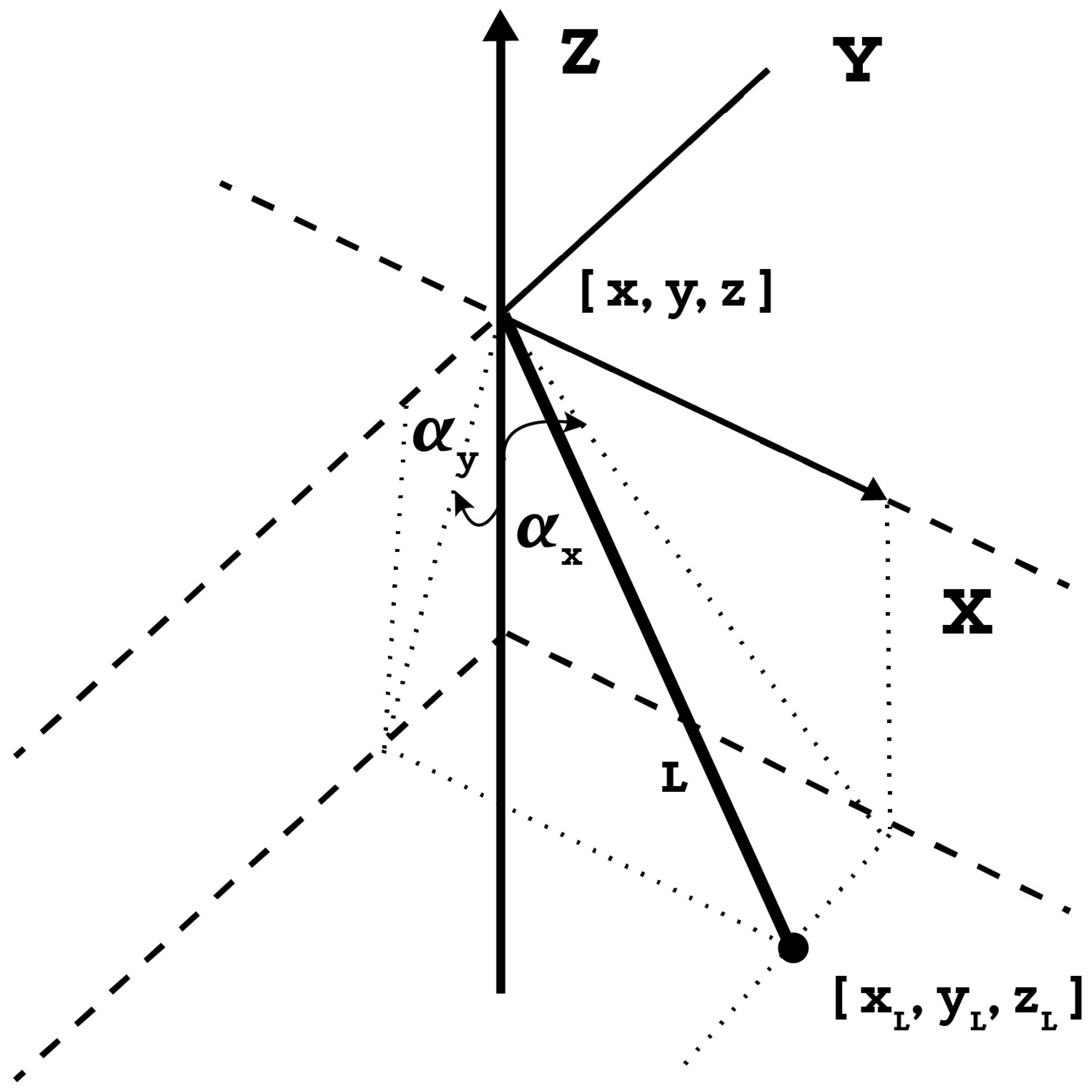
As seen in
Figure 2, where the payload was modeled as a three-dimensional point pendulum mass, the equations defining the dynamics of the load were derived by taking into account the
longitudinal suspension angles in the
plane and the
longitudinal angles and forces in the
plane. The following are the forces generated by the load on the respective axes [
46]:
where
is the payload’s mass;
are the payload’s forces effect on quadrotor in three-dimensional space shown in
Figure 2.
Hence, the entire system dynamics are as follows:
2.4. Neural Network
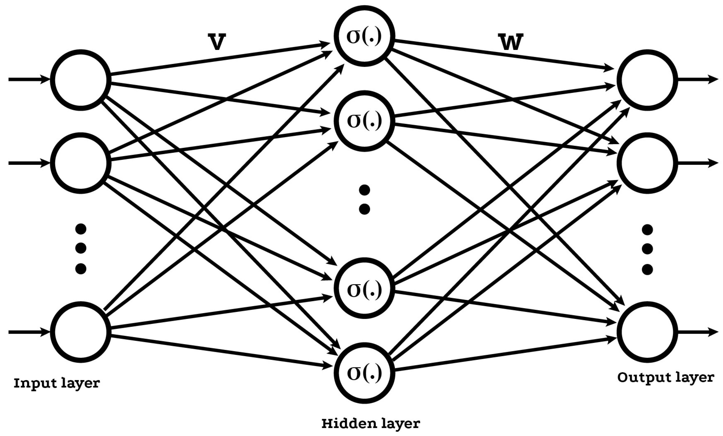
In this work, a two-layer neural network (NN) structure was used to estimate uncertain dynamics as shown in
Figure 3.
The first layer is hidden and contains adjustable hidden weights,
, and the second layer consists of randomly determined constants,
where
is the input count and
is the output count.
represents the number of neurons in the hidden layer. Estimation function
can be given as
where
is the bounded NN estimation error that satisfies
, and
is the activation function for the hidden layer. Because input-layer weights
are randomly chosen, for any input
x, the estimation is viable; hence, activation function,
, establishes a stochastic base in compact set
S [
47].
, where
is a bias term of input that lets threshold value to be in weight matrix
. As an activation function, a tangent hyperbolic function in the form of
, was chosen in this study for all neurons. It was also assumed that target weights were limited to a known positive value
satisfying
on any compact subset of
[
48]. Moreover,
and
are considered as the vector and Frobenius norm, respectively [
47].
Next, the controller design is given.
3. Controller Design
The suggested controller is outlined here. The proposed controller takes into consideration quadrotor dynamics, and the unpredictable dynamics caused by external disturbances and parametric uncertainties. To reduce the chattering influence of the SMC, the unknown dynamics are learned using two-layer NN. Because of the neural-network component, the controller can successfully govern the system without understanding the quadrotor dynamics. Furthermore, utilizing the updated learning structure, system dynamics may be appropriately updated even when there are uncertainties that change over time. With the assistance of a finite-time control system, the trajectory errors converge to zero in a finite time.
To enable effective controller design, the dynamic equations obtained in (
9) are subjected to the following transformation [
45]:
where
Moreover, sliding surface functions are selected as follows [
49,
50]:
where
,
, and
are the coefficients of sliding surfaces that are described later.
is the representation of
where
.
3.1. Coefficients of Sliding Surfaces
The coefficients of the sliding manifolds in (
12) are derived using the same Hurwitz stability criterion as in [
45,
51], and they are provided as follows:
where
are the design parameters that are constant.
3.2. Ftnsmc Controller Design
In real-world systems, neural networks (NNs) are always used as one of the online estimation methodologies for dealing with unknown nonlinear uncertainties. The nonlinear quadrotor dynamics in (
10), including parametric uncertainties and external disturbances, are considered to be unknown in this section. Unknown nonlinear dynamics
are estimated as follows:
where
are the required limited NN weights meeting
and
is a positive constant,
represents the positive NN learning rate that is specified later,
is the number of neurons in the hidden layer,
represents the basis function, and
represents the mapping between the inputs and the hidden-layer neurons, where
is the number of inputs to the NN,
with
being a positive constant, and
being the limited NN reconstruction error fulfilling.
represents the unknown NN weights, and the approximated uncertain dynamics are given by:
The NN weight estimation error is defined as
, and the estimation error dynamics are
. The error in dynamics estimation can, therefore, be described as follows:
The estimated NN weights were adjusted using the adaption law shown below:
where
is the learning rate.
An exponential reaching law is provided to achieve appropriate steady-state behavior [
52]:
where
,
and
.
Taking the derivative of sliding surface
defined in (
12) yields:
The dynamics of the system, including parametric uncertainties and external disturbances, were considered to be unknown and they were estimated with the NN in this work. Therefore, by inserting the estimation function in (
16) for all the dynamics, and taking the reaching law into consideration in (
18) for
control signals can be written as follows:
3.3. Stability Analysis
Theorem 1. Consider nonlinear System (10) with the sliding surface dynamics in (19), the controller inputs as in (20), and the estimated dynamics applied to the system, and the estimated NN weights tuned with the adaptation law (17), All NN weight estimation errors and sliding surfaces were SGPFS, and the tracking error converged in a finite time to a small neighborhood of the origin. Proof of Theorem 1. Define the Lyapunov candidate function of all sliding surfaces,
and NN weight estimation errors
as follows:
by taking Derivative (
21) and inserting the dynamics in (
10), and considering that
to obtain:
Using the controller inputs in (
20), dynamic estimation error function in (
16) and reaching law in (
18), (
22) can be rewritten in a compact form as:
The following inequalities hold from Young’s inequality in Lemma 3:
Upper bounds
and
; inserting (
24) into (
23), we obtain:
Here, by using Lemma 2, the inequality below holds:
Moreover, according to Lemma 4, the inequalities. below exist:
where
.
By using (
26) and (
27), and Lemma 2, (
25) can be rewritten as:
where
,
, with .
Now let
With Lemma 1, all signals are SGPFS,
,
.
Moreover, from the definition of
V,
, the following can be obtained:
After a finite time , the tracking errors of all states converge to a small neighborhood of the origin and stay there. This concludes the proof. □
Remark 1. According to stability analysis, design parameters , and significantly impacted the proposed controller’s capacity for stability. High control precision and a quick convergence rate can result from large . They could, however, provide comparatively huge control torques that would not be practical. High control precision and a quick convergence rate can also come from large . This might, however, potentially cause an infinite convergence. Therefore, it is important to carefully choose the design parameters of the suggested controller so that it can reach a sufficient level of control performance.
Remark 2. Due to their fractional power structure, finite-time-based controllers are more reliable than traditional controllers, as is demonstrated in the simulation results in the next section. However, because initial conditions impact the convergence time of the finite-time controller, this is not always possible in applications. Therefore, it is not always possible to compute the settling time of the finite-time controller. Since the estimated function’s initial values are included in this study, it is also not possible to accurately compute the settling time. A fixed-time stability structure was suggested in the literature [53] as a solution to this issue, and this structure may serve as the subject of our next research. Next, numerical simulations are given in detail.
4. Numerical Simulations
To test the efficiency of the suggested controller, a nonlinear model of a quadrotor UAV was built and simulations in MATLAB were run; ode45 was used as the solver. Two different trajectory tracking simulations were performed on quadrotor UAV transporting a suspended payload system to demonstrate the effectiveness of the developed controller. Furthermore, the simulations were enlarged with two more control approaches, demonstrating the superiority of the suggested control over other control structures. First, a classical SMC was used to control the system. Then, the system was controlled with a finite-time SMC (FTSMC) control structure by adding a finite-time control structure to the classical SMC structure. Thus, before adding the neural-network component, the advantages of the finite-time control structure over the classical SMC were observed. Lastly, we clearly demonstrate the superiority of the results obtained using the proposed controller, finite-time-based neuro-sliding mode controller (FTNSMC) over the results obtained in the previous simulations.
The parameters of the quadrotor dynamical model are given in
Table 1. The UAV’s mass and inertia were also subject to a
uncertainty as
,
,
,
. Moreover, the quadrotor was assumed to be subjected to constant time-varying disturbances as
,
,
,
,
,
,
. Moreover, payload’s desired angles are chosen as,
,
, where
. Controller parameters were selected by trial and error as in
Table 2. The hidden-layer neurons were employed at random, while the neural-network weights were initially set to zero during the simulations. The simulations were run with the following assumptions in mind.
Assumption 1. The parametric uncertainties and external disturbances that were defined in (9) were assumed to be bound by a known bound.where , and it was taken to be in the simulations. Assumption 2. The parametric uncertainties and external disturbances that were defined in (9) were assumed to be bounded by a known bound. Two different scenarios were considered in the simulations for the trajectory tracking problem of quadrotor carrying a suspended payload.
4.1. Scenario 1
In the context of model uncertainties and external disturbances, the control goal was to allow the quadrotor to track a square desired trajectory. For simulation experiments, the quadrotor’s beginning position and angle parameters were
and
, and the chosen desired quadrotor trajectories are listed in
Table 3. The simulation time for all runs was 80 s.
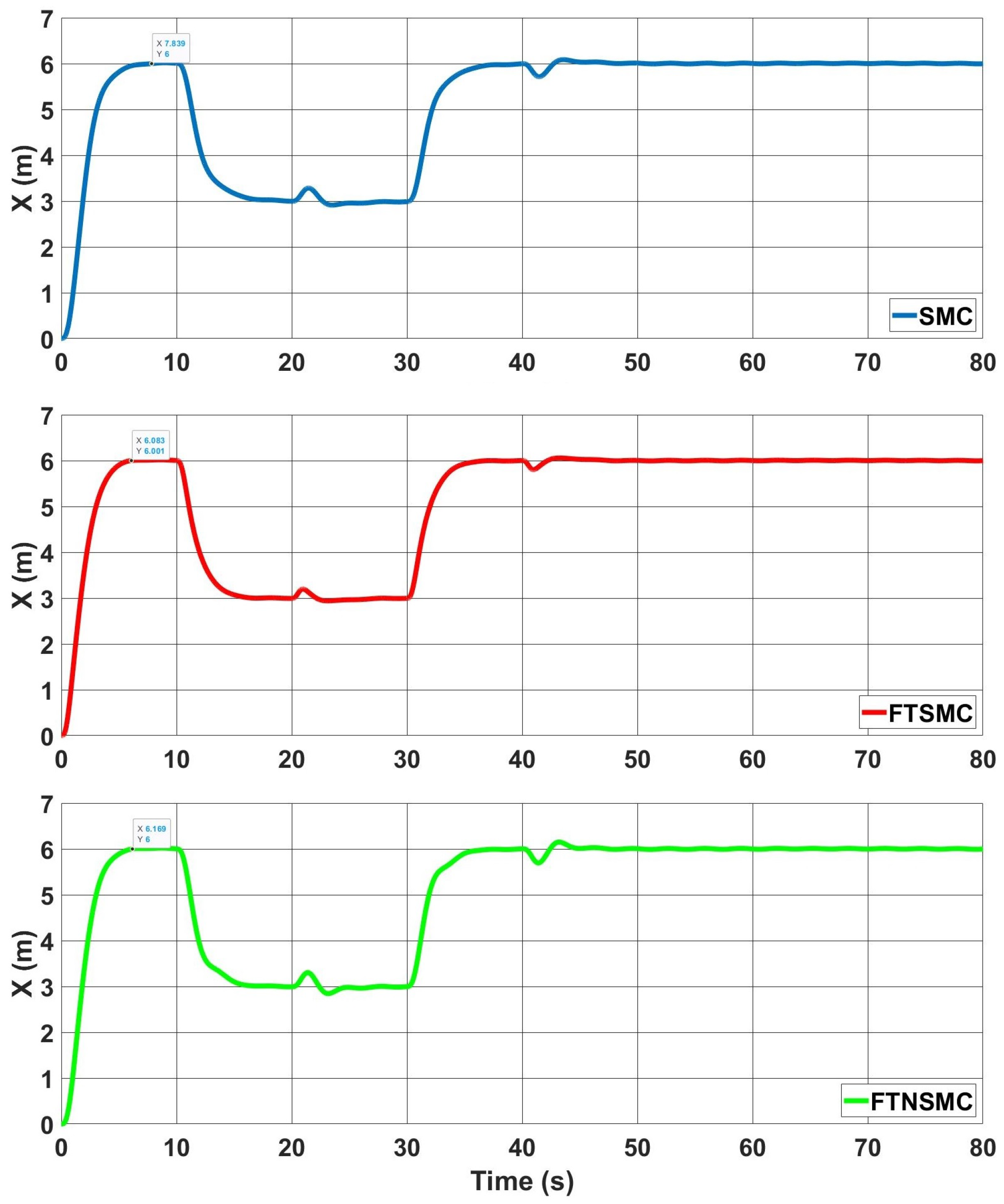
The
x position of the quadrotor for three controllers is given in
Figure 4. For a classical SMC, the quadrotor reached the first desired
x value at around 7.89 s. The addition of a finite-time structure decreased the reaching time to around 6.08 s, and with the proposed method, the quadrotor reached the first desired
x value at around 6.16 s.
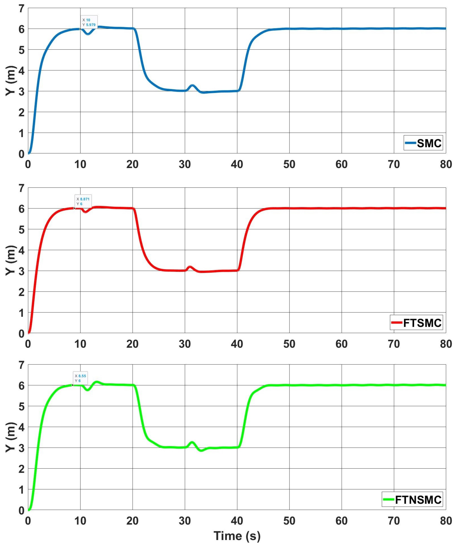
The
y position of the quadrotor for three controllers is given in
Figure 5. For a classical SMC, the quadrotor could not reach the first desired
y value but it reaches about 5.97 m at 10 s. With FTSMC, the quadrotor reached the first desired
y value at around 8.87 s, and with the addition of the neural-network component, this value decreased to around 8.55 s.
The
z position of the quadrotor for three controllers is given in
Figure 6. The quadrotor arrived at the desired 6 m value at around 12.68 s, whereas for FTSMC, this value decreased to 10.53 s; with the suggested controller, it settled to the desired value in less than 8.46 s.
In
Figure 7, the change in controller input
is given. Although the initial values of the control input were similar in all three controllers, the chattering effect was clearly observed for the classical SMC. With FTSMC, this chattering decreased but remained. Using the proposed controller, the chattering effect completely disappeared. Moreover, the proposed controller exceptionally decreased the input value compared to SMC and FTSMC.
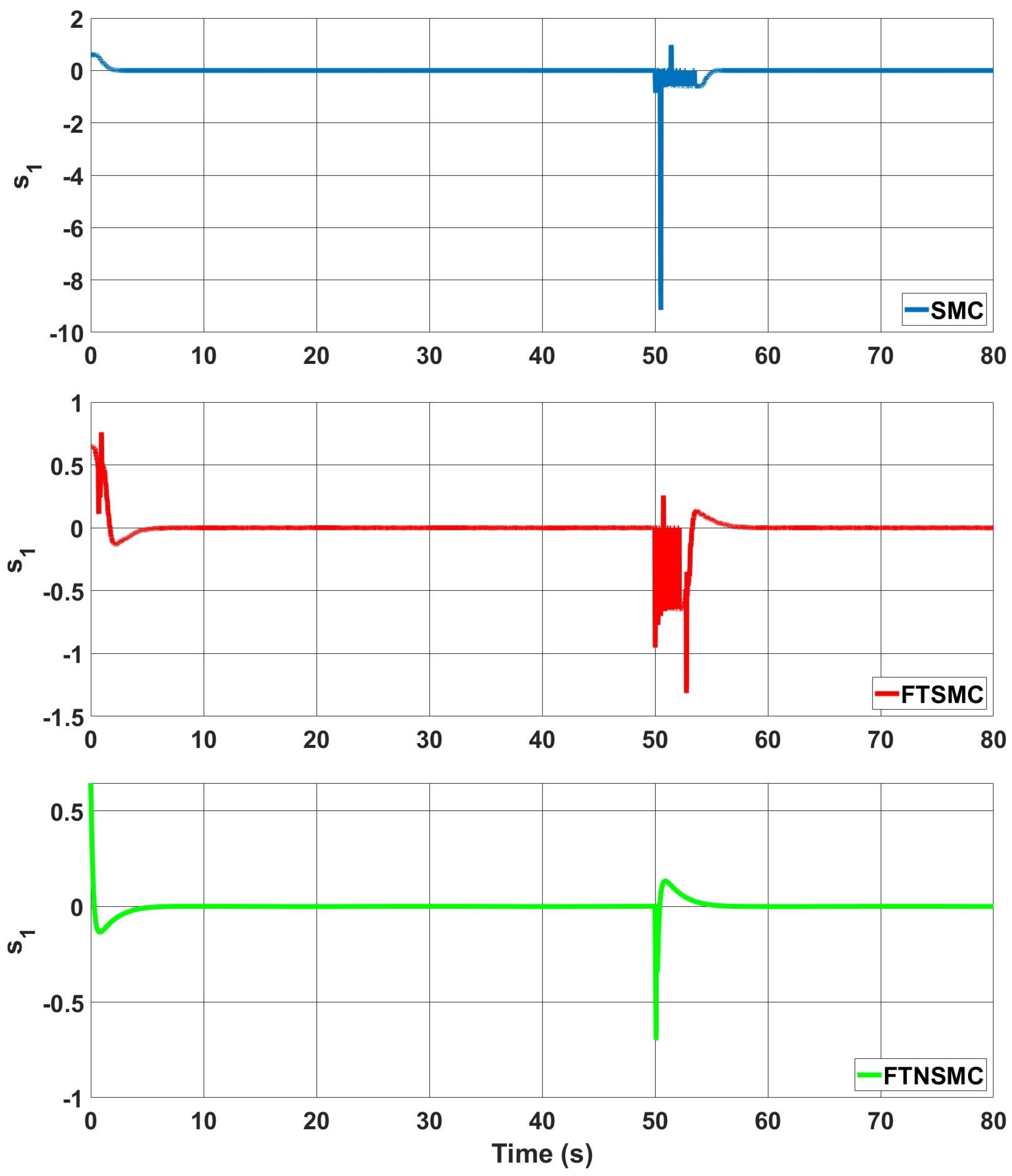
Figure 8 displays the change in sliding variable
. It behaved as expected when the variables approached its sliding surfaces. Additionally, the oscillations of the sliding variable completely accounted for the position and velocity tracking inaccuracies of the system state variables.
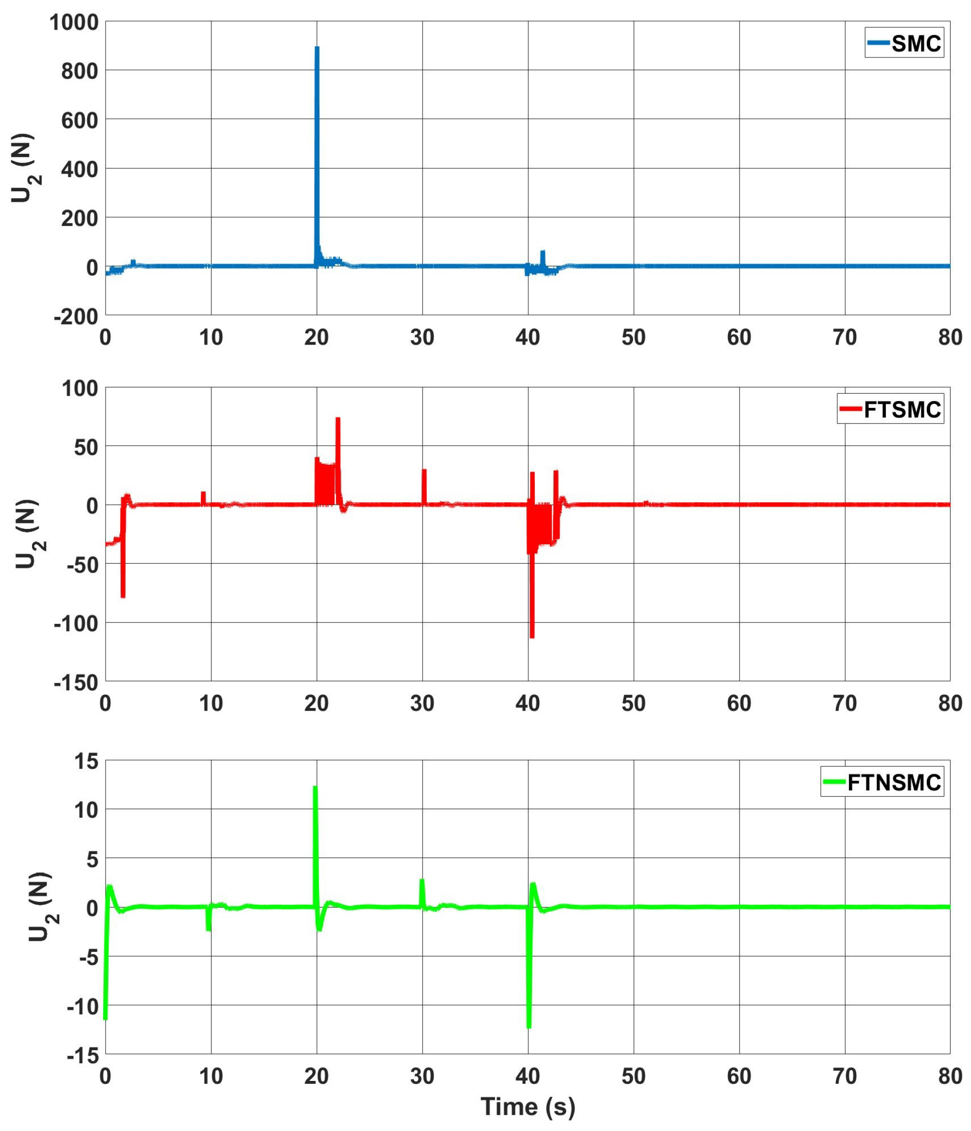
Variation in controller inputs
and
is seen in
Figure 9 and
Figure 10 respectively. Ẇhen SMC was used, both a chattering effect and a very high control input value were observed. By adding finite time to SMC, the chattering decreased as the value of the control input decreased with FTSMC. However, in both cases, high sparks and chattering could be seen clearly. Using the proposed controller not only significantly reduced the value of the control input, but also completely eliminated the chattering effect.
In
Figure 11, the change in controller input
is given. Despite the fact that the starting values of the control input were comparable in all three controllers, the chattering effect was plainly seen in the conventional SMC. This chattering was reduced by FTSMC, but it still existed. When the proposed controller was used, the chattering effect was fully eliminated.
Variations in quadrotor angles for proposed controller are given in
Figure 12.
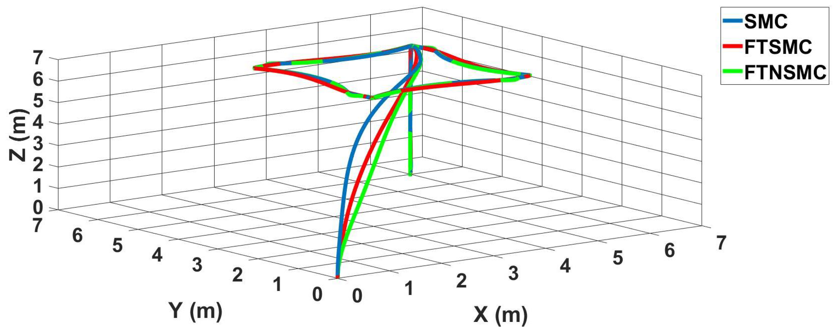
The trajectory tracking of the UAV in 3D is given in
Figure 13 for all three controllers. Adding a finite-time structure to the conventional SMC obviously sped up the system responsiveness. Additionally, the NN improved the system response even more.
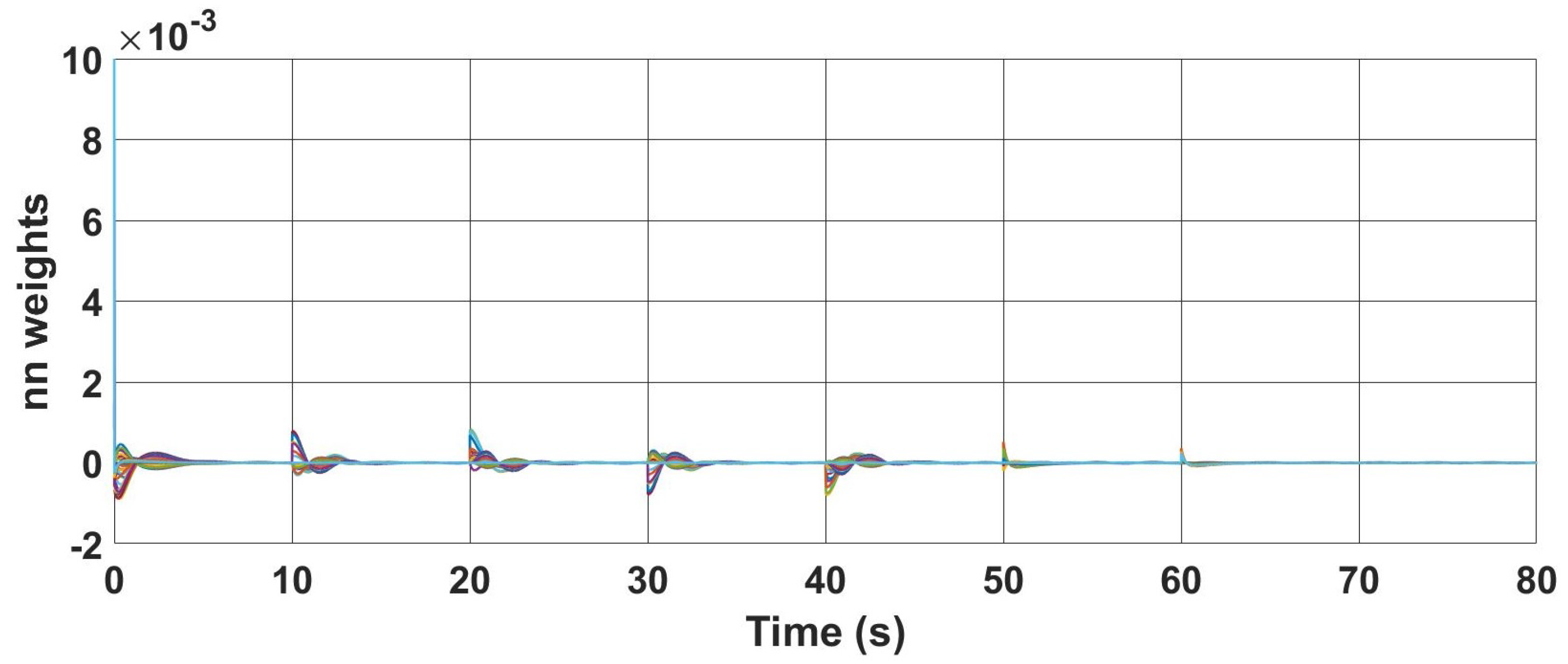
Figure 14 shows the variation in the neural-network weights. As expected, the neural-network weights rapidly learnt the unknown dynamics after each movement of the UAV and converged to a value close to zero.
4.2. Scenario 2
In the second simulation, the control goal was to allow the quadrotor to track a circular desired trajectory and also ensures that the system state errors reach zero or to a close neighbourhood of zero in a finite time. The chosen desired quadrotor trajectories are listed in
Table 4. The simulation time for all runs was 320 s.
The errors in the
x axis for three controllers are given in
Figure 15. Compared to a classical SMC, the proposed controller provided a fast convergence rate as accepted. The error in the
x axis reached zero for the first time at around 4.3 s with the proposed controller and oscillated in the neighborhood of zero with a small margin because of the nature of desired trajectory, whereas it reached zero at around 6.6 s with FTSMC and 14 s with classical SMC.
Figure 16 displays the
y-axis errors for three controllers. With the SMC, error convergence was very slow and it converged to zero after 50 s, as seen in the figure. The addition of finite-time structure decreased this value to around 13 s.
In
Figure 17 errors in the
z axis are shown. For SMC controller error reached the neighborhood of zero within around 6.5 s. With FTSMC, this value was around 5.5 s, and with FTNSMC, it was around 4.5 s.
controller inputs for three controllers are given in
Figure 18. Since the desired trajectory was orbital, the progress of the motion in the
z axis was expected to be slow. Changes in the control inputs for this axis were, therefore, close to each other within the three controllers. On the other hand, there was a difference between the convergence of the control inputs to nominal value. This time was around 4.5 s for SMC and FTSMC, and this time decreased to 2.8 s for the proposed controller. Moreover, small chattering could be detected with FTSMC, but this effect was also eliminated with FTNSMC.
Variations in control inputs
and
are given for the three controllers in
Figure 19 and
Figure 20, respectively. The control signal for SMC exhibited undesirable sparks at the beginning with some chattering effect and, since it could only enter the desired trajectory after 50 s, high chattering occurred at these time values for input
. FTSMC reduced this chattering effect while increasing the initial value of control input; lastly, by using NNFTSMC, a chattering-free control input could be obtained while decreasing the initial value of control input of FTSMC. For the
control input, a chattering effect could also be seen for SMC and FTSMC. However, the neural-network component in the proposed controller significantly reduced this effect.
Figure 21 demonstrates the change of control inputs
for the three controllers. Although the initial values were close to each other for all controllers, with the proposed controller, the control input converged to zero more quickly after the initial movement and it was a smoother control input than the SMC and FTSMC methods. Furthermore, FTSMC showed more chattering-free control input behavior than the classical SMC did.
In
Figure 22, the trajectory of the quadrotor in 3D space is given for three controllers. The suggested controller tracking performance of the desired trajectory was superior to that of classical SMC and FTSMC.
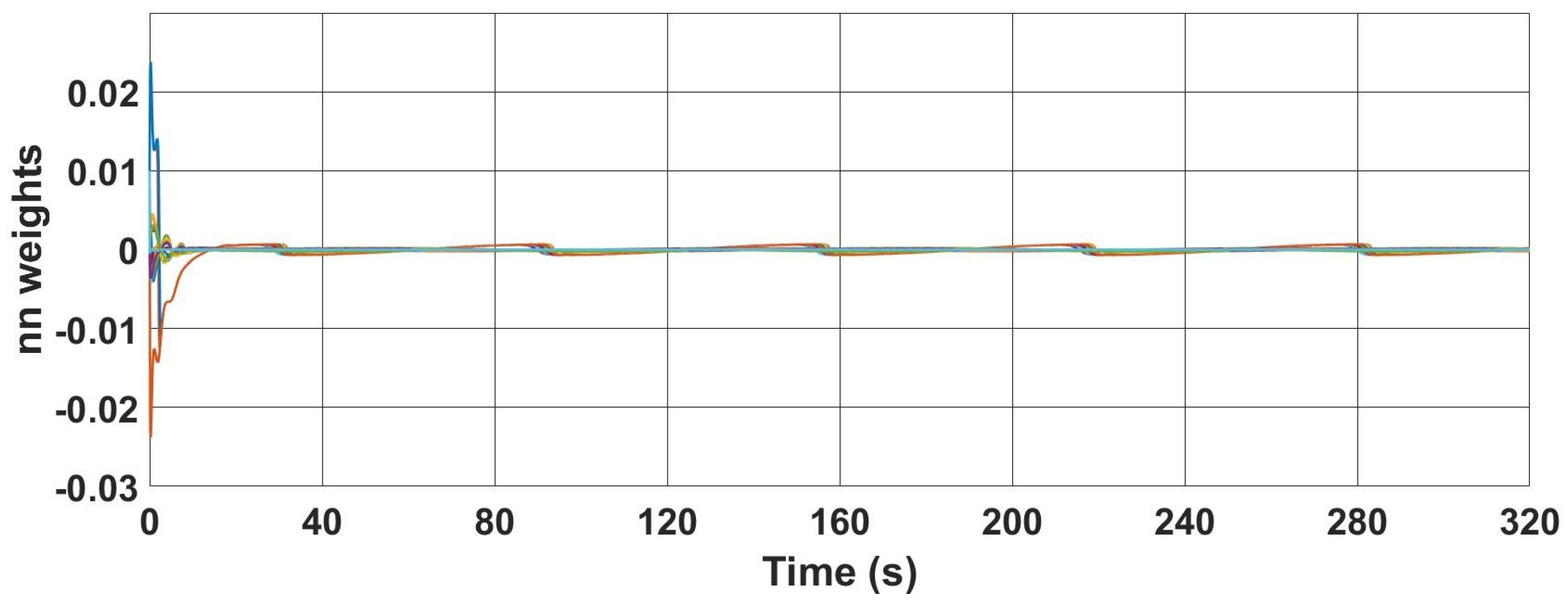
The change in neural-network weights is presented in
Figure 23. As expected, the neural-network weights rapidly learnt the unknown dynamics after each movement of the UAV and converged to a value close to zero.
5. Conclusions
A neural-network-based finite-time sliding-mode controller was proposed to control a quadrotor UAV carrying a suspended payload with parametric uncertainties and external disturbances. After deriving the full nonlinear mathematical model of system, the proposed controller was developed, and three different simulations were performed to demonstrate the effectiveness of the proposed controller. First, the system was controlled with a classical SMC. In this simulation, errors in the trajectory tracking in all three axes due to the effects of unknown dynamics and serious chattering effects were observed in the control signals. Very high control signals were also needed to control the system. In the second simulation, a finite-time control structure was added to the SMC to reduce the values of the control signals and the trajectory tracking errors to converge to zero in a finite time. Although FTSMC improved the settling times and the values of the controller signals, it was not effective in eliminating the chattering effect. A neural-network structure was added to FTSMC to construct the proposed controller and effectively handle chattering. With the use of the neural network, chattering disappeared completely, the control signs were significantly reduced, and the settling times were further improved. Future work is to improve the finite-time stability to fixed-time stability to be able to free it of initial conditions to calculate the reaching time, demonstrating the effectiveness of the proposed controller with a real-time experiment.


